Robust Bi-Orthogonal Projection Learning: An Enhanced Dimensionality Reduction Method and Its Application in Unsupervised Learning ^†

Abstract

This paper introduces a robust bi-orthogonal projection (RBOP) learning method for dimensionality reduction (DR). The proposed RBOP enhances the flexibility, robustness, and sparsity of the embedding framework, extending beyond traditional DR methods such as principal component analysis (PCA), neighborhood preserving embedding (NPE), and locality preserving projection (LPP). Unlike conventional approaches that rely on a single type of projection, RBOP innovates by employing two types of projections: the “true” projection and the “counterfeit” projection. These projections are crafted to be orthogonal, offering enhanced flexibility for the “true” projection and facilitating more precise data transformation in the process of subspace learning. By utilizing sparse reconstruction, the acquired true projection has the capability to map the data into a low-dimensional subspace while efficiently maintaining sparsity. Observing that the two projections share many similar data structures, the method aims to maintain the similarity structure of the data through distinct reconstruction processes. Additionally, the incorporation of a sparse component allows the method to address noise-corrupted data, compensating for noise during the DR process. Within this framework, a number of new unsupervised DR techniques have been developed, such as RBOP_PCA, RBOP_NPE, and RBO_LPP. Experimental results from both natural and synthetic datasets indicate that these proposed methods surpass existing, well-established DR techniques.

1. Introduction

The curse of dimensionality represents a widespread hurdle in numerous real-world scenarios, particularly in applications involving high-dimensional data like facial and textual images. This problem can significantly hinder the efficacy of subspace learning methodologies owing to their excessive computational expenses and considerable memory demands. DR is crucial for tackling this issue, as it strives to preserve essential characteristics of the data in a lower-dimensional space. Since high-dimensional data typically arise from an underlying low-dimensional manifold structure [1]; the objective of DR is to reveal these informative, compact, and meaningful low-dimensional structures that are embedded within the original high-dimensional space. This promotes enhanced classification and visualization capabilities [2,3,4]. The desired attributes are usually specified by an objective function, and the task of DR can be formulated as an optimization problem [5].

DR methods are generally divided into three types according to the label information used for training samples: supervised, semi-supervised, and unsupervised DR. Supervised DR methods leverage label information to learn a projection that enhances class discrimination. Notable examples include linear discriminant analysis (LDA) [6,7], local linear discriminant analysis (LLDA) [8], sparse tensor discriminant analysis (STDA) [9], locality sensitive discriminant analysis (LSDA) [10], discriminative locality alignment (DLA) [11], marginal Fisher analysis (MFA) [12], and local discriminant embedding (LDE) [13]. Each of these techniques has unique strengths, depending on their specific focus. LDA is a fundamental method, while LLDA, an extension of LDA, emphasizes the local separability between different classes, although it still faces the small-sample-size problem and handles intra-class data similarly to LDA. LLDA specifically concentrates on classes that are spatially proximate in the data space, with the assumption that this closeness enhances the probability of misclassification. Consequently, its objective is to optimize the separation between adjacent classes. LSDA endeavors to maximize the margins between distinct classes within every local region. It aims to project samples of the same class, which are neighboring in the high-dimensional space, to be nearer in the reduced space, while making sure that samples from various classes are distinctly separated, thus increasing the discriminative ability in the lower dimensions. DLA is designed to handle nonlinearly distributed data, preserving local discriminative information and avoiding issues with matrix singularity. MFA, on the other hand, is a linear feature extraction technique based on the Fisher criterion within a graph embedding framework. LDE prioritizes the local and class relationships among data points, preserving the internal proximity of points belonging to the same class while guaranteeing that points from distinct classes are not adjacent in the embedded space, thus enhancing class distinction.

The aim of DR techniques is to identify a discriminative projection that concurrently maximizes the separations between the centroids of distinct classes and reduces the proximity of data points belonging to the same class, employing Fisher’s criterion [8]. However, high-quality labeled data are often scarce compared to the abundance of unlabeled data [14]. Unlabeled data can be valuable for enhancing algorithm performance. Semi-supervised DR methodologies take advantage of the distribution and local structure of both labeled and unlabeled data, together with the labeling information from the labeled data, to boost performance. Semi-supervised discriminant analysis (SDA) strives to identify a discriminative projection that maximizes the separability of labeled data across distinct classes while estimating the intrinsic geometric structure of the unlabeled data [15]. SDA makes use of both labeled and unlabeled samples. labeled samples serve to boost the separability among distinct classes, while unlabeled samples contribute to delineating the underlying data geometry. The objective is to learn a discriminant function that represents the data manifold as smoothly as possible. Constrained non-negative matrix factorization (CNMF) has been proposed to address the limitations of the original non-negative matrix factorization (NMF), which does not incorporate label information [16]. CNMF purposefully employs the label information from the labeled samples to bolster the discriminative strength of the matrix decomposition. The label information is implemented as an extra hard restriction, ensuring that data points sharing the same label maintain their coherence in the newly reduced dimensional space. However, since there are no constraints on the unlabeled data, the performance of CNMF can be limited when the amount of label information is minimal. In cases where only one sample per class is labeled, the constraint matrix in the algorithm effectively becomes an identity matrix, rendering it ineffective.

Unsupervised DR methods aim to preserve the intrinsic manifold structure of the data by exploring the local relationships between data points and their neighbors. Key examples of such methods include locally linear embedding (LLE) [17], Laplacian Eigenmaps (LEs) [18], neighbor preserving embedding (NPE) [19], orthogonal neighborhood preserving projection (ONPP) [20], and locality preserving projection (LPP) [21]. The LLE method [17] is particularly effective for data with an overall nonlinear distribution, as it has a strong capability to maintain the original data structure, even for datasets with complex nonlinear structures. Similarly, LEs [18] reconstruct the local structure of the data manifold by establishing a similarity graph, which effectively captures the intrinsic manifold structure. NPE [19] focuses on preserving the locally linear structure of the manifold during the dimensionality reduction process, allowing it to extract useful information from the data. This method can capture both the nonlinear structure of manifolds and retain linear properties, making it suitable for generalization to new samples. Both ONPP [20] and the LPP method [21] employ learned projections to reduce the dimensionality of data in a space. These methods model the data manifold using a nearest-neighbor connection graph, which preserves the local structure of the data. The resulting projection subspaces are intended to maintain the nearest-neighbor associations, guaranteeing that the local geometry of the data is preserved within the reduced space.

Recently, Wang [12] introduced a new graph embedding framework that unifies various DR methods, including LDA, ISOMAP, locally linear embedding (LLE), Laplacian Eigenmaps (LEs), and LPP. In this framework, the statistical and geometric properties of the data are encoded as graph relationships. PCA [22] is a widely recognized method that maps high-dimensional data onto a lower-dimensional space by identifying the directions of maximum variance for optimal data reconstruction. Modified principal component analysis (MPCA) enhances PCA by employing various similarity metrics to more accurately capture the similarity structure of the data [23], and sparse PCA (SPCA) [24] has been introduced. From the overview of the three categories of DR methods, supervised, semi-supervised, and unsupervised, it is evident that obtaining labeled data samples in real-world scenarios can be costly and challenging. Therefore, this paper focuses on unsupervised DR methods. Nevertheless, current unsupervised DR techniques might possess the following possible disadvantages:

(1) Many unsupervised DR methods, such as LPP and NPE, rely on the similarity matrix (or affinity graph) of the input data. As a result, the quality of subspace learning is significantly influenced by the construction of this affinity graph. Furthermore, since similarity measurement and subspace learning are typically conducted in two distinct stages, the acquired data similarity may not be optimal for the subspace learning task. This can result in sub-optimal performance.

(2) These approaches generally learn just one projection throughout the dimensionality reduction procedure. This singular projection provides limited adaptability for attaining a more precise data transformation, which may result in a less effective representation within the lower-dimensional space.

To tackle these challenges, this paper introduces a new learning approach, RBOP, which is an extension of our previous work [25]. In contrast to conventional methods that necessitate a similarity matrix of the data as input, RBOP employs sparse reconstruction to guarantee that the projected data retain sparsity, as shown in Figure 1. The sparse reconstruction coefficient matrix serves to encode the local geometric characteristics of the data, effectively fulfilling the role of a similarity matrix. Through this method, the similarity matrix can be directly learned throughout the dimensionality reduction procedure. In contrast to traditional DR techniques that depend on a single projection, RBOP employs two separate projections: the “true” projection and the “counterfeit” projection. These two projections are orthogonal to one another. The “true” projection is afforded considerable latitude, allowing it to learn a more precise and effective data transformation. This dual-projection methodology boosts the adaptability and resilience of subspace learning, ultimately resulting in improved representation within the lower-dimensional space.

Moreover, drawing inspiration from the observation that the two projections exhibit a similar data structure, we stipulate that the data projected by these two techniques maintain this structural resemblance via two distinct reconstruction methodologies. We incorporate a sparse term for error compensation, which helps in learning robust projections by mitigating the impact of noise. This sparse term weakens the response to noise during the learning process, thereby enhancing the robustness of the projections. The proposed RBOP approach has the potential to expand several unsupervised dimensionality reduction methods into a robust and sparse embedding framework for subspace learning. We have devised an efficient and effective algorithm to address the optimization problem that arises. The efficacy of RBOP is substantiated by remarkable experimental outcomes, which exhibit considerable enhancements compared to prevailing methods.

This paper presents the following principal contributions:

(1) For the first time, we propose a novel concept and methodology for learning bi-orthogonal projections in the context of DR. Utilizing the inexact augmented Lagrange multiplier (iALM) technique as a foundation, we develop an efficient algorithm to tackle the optimization problem that ensues. Both theoretical validations and empirical assessments substantiate the effectiveness of the devised optimization algorithm.

(2) We approach the DR challenge from a fresh viewpoint by concurrently acquiring the data similarity matrix and the subspace via sparse reconstruction and the learning of two orthogonal projections. This methodology guarantees the preservation of the local geometric structure of the data while capitalizing on the complementary insights offered by the two projections.

(3) By employing the proposed RBOP, we extend several conventional DR methods into a robust and sparse embedding framework. This extension bolsters the resilience of these methods against various kinds of noisy data and allows them to learn more precise and meaningful subspaces.

The rest of this paper is structured in the following manner. In Section 2, we conduct a comprehensive review of the existing literature and related studies. In Section 3, we introduce the proposed theoretical framework and formulation. This is succeeded by a detailed examination of the optimization algorithm, computational complexity, and convergence analysis in Section 4. To validate the efficacy of our approach, we present empirical results in Section 5, which demonstrate the effectiveness of the proposed method. Lastly, we wrap up our discussion and draw conclusions in Section 6.

2. Related Work

This section provides a concise overview of the pertinent research on various established DR techniques, such as PCA, LPP, and NPE. Subsequently, we illustrate that these conventional methodologies can be restructured within a cohesive framework, thereby simplifying the representation and comprehension of our proposed robust bi-orthogonal projection (RBOP) approach.

2.1. PCA

PCA [22] is a commonly used unsupervised DR technique that seeks to identify a projection direction that maximizes the variance of the data. The variance of the projected data can be re-expressed as ${\sum }_{i=1}^n{\sum }_{j=1}^n{\parallel W^T{x}_i-W^T{x}_j\parallel }_2^2=tr\left(W^{T}XH{X}^{T}W\right)$, where H is the centering matrix, which can be represented as $H=I-{\displaystyle \frac{1}{n}}\mathbf{1}{\mathbf{1}}^T$; 1 is a vector with all elements are 1. It is obvious that the variance of the centering data is $-XH{X}^T=\mathrm{\Sigma }$. Therefore, PCA determines the projection matrix W by addressing the following problem:

$$W^{*}=\underset{W^{T}W=I}{argmin}tr\left(W^T(\mathrm{\Sigma }-uI)W\right)$$

(1)

2.2. LPP

LPP [21] initially learns an affinity graph $\mathcal{S}$ that depicts the pairwise relationships among data points. Subsequently, it searches for a “superior” mapping that ensures data points in the desired low-dimensional subspace can effectively maintain their locality. LPP determines the projection matrix W by solving the following problem:

$$W^{*}=\underset{W^{T}XD{X}^{T}W=I}{argmin}\sum _{i=1}^n\sum _{j=1}^n{\parallel W^T{x}_i-W^T{x}_j\parallel }_2^2{\mathcal{S}}_{ij},$$

(2)

where D is the degree matrix of $\mathcal{S}$.

There is another variant of LPP [20] which is as follows:

$$\begin{array}{cc}\hfill W^{*}& =\underset{W^{T}W=I}{argmin}\sum _{i=1}^n\sum _{j=1}^n{\parallel W^T{x}_i-W^T{x}_j\parallel }^2{\mathcal{S}}_{ij}\hfill \\ \hfill & =\underset{W^{T}W=I}{argmin}tr\left(W^{T}XL{X}^{T}W\right)\hfill \\ \hfill & =\underset{W^{T}W=I}{argmin}tr\left(W^T(\mathrm{\Sigma }-uI)W\right),\hfill \end{array}$$

(3)

where $L=D-\mathcal{S}$ ($\mathrm{\Sigma }=XL{X}^T$) is a graph Laplacian and $D_{ii}={\sum }_j{\mathcal{S}}_{ij}$.

2.3. NPE

NPE strives to maintain the local neighborhood structure of data [19]. Initially, NPE constructs an affinity graph, followed by utilizing the local approximation error to compute the weights of the graph:

$$\begin{array}{cc}\hfill {\mathcal{S}}^{*}& =argmin\sum _{i=1}^n{\parallel x_i-\sum _j{\mathcal{S}}_{ij}{x}_j\parallel }^2\hfill \\ \hfill s.t.& \sum _j{\mathcal{S}}_{ij}=1,j=1,2,...,n.\hfill \end{array}$$

(4)

Finally, NPE computes the projection matrix W by solving the following problem:

$$\begin{array}{cc}\hfill W^{*}& =\underset{W^{T}W=I}{argmin}tr\left(W^{T}X{(I-\mathcal{S})}^T(I-\mathcal{S})X^{T}W\right)\hfill \\ \hfill & =\underset{W^{T}W=I}{argmin}tr\left(W^{T}XM{X}^{T}W\right)\hfill \\ \hfill & =\underset{W^{T}W=I}{argmin}tr\left(W^T(\mathrm{\Sigma }-uI)W\right),\hfill \end{array}$$

(5)

where $M={(I-\mathcal{S})}^T(I-\mathcal{S})$ and $\mathrm{\Sigma }=XM{X}^T$.

3. Robust Bi-Orthogonal Projection Learning

This section provides a detailed explanation of the proposed RBOP methodology, accompanied by its respective optimization algorithm and an extensive algorithmic analysis. Despite the multitude of methods that have been put forward for DR stemming from various motivations, they all share a common objective: to streamline subsequent data analysis tasks, including classification and clustering, by obtaining a low-dimensional representation of the data. With this in mind, we integrate these disparate DR methods into the RBOP framework.

3.1. Motivations of RBOP

From the above deductions, we can see that (1) it is still necessary to construct an affinity graph ahead of time to serve as the input for methods such as LPP, NPE, DLA, and MFA. This renders DR significantly reliant on the quality of the data similarity matrix to a great extent. (2) These methods merely learn a single projection W, which is responsible for both preserving the structural information encoded by the affinity graph and projecting the data into a low-dimensional subspace. This dual-purpose requirement, or “mind bent on dual-use”, limits the freedom of W to learn a more accurate transformation for the dataset. (3) These methods assume the input data to be noise-free. Consequently, they experience significant performance degradation when noisy data are present. Despite their obvious importance, these three problems of conventional DR methods have been relatively unexplored in the community of subspace learning. Recent research [23,26] indicates that an ${\ell }_1$ graph [27] can capture the similarity structure of the data well.

Moreover, an ${\ell }_1$-norm-based sparse matrix can enhance the robustness of the algorithm [23]. Therefore, introducing them to our method will likely be an excellent choice to accomplish the desired purpose. Further, the data similarity matrix and subspace learning are performed simultaneously, which seems to achieve optimal results for DR and the affinity graph. Additionally, to acquire a more precise transformation, we naturally take the single projection used in conventional DR methods and replace it with double projections, thus avoiding the problem of “mind bent on dual-use”. Based on the above considerations, we propose a novel robust bi-orthogonal projection learning method to address these three problems in the following subsection.

3.2. The Objective Function of RBOP

Given data $X\in {\Re }^{m\times n}$, where m and n are the number of dimensions and data points, respectively, we aim to learn two distinct orthogonal projection matrices $P\in {\Re }^{m\times d}$ and $W\in {\Re }^{m\times d}$ (d denotes the dimensionality of the reduced subspace) such that the “true” projection matrix W enjoys greater flexibility in transforming the data into a more precise subspace, effectively preserving the similarity structure of the data. To achieve this, we propose the following objective function:

$$\begin{array}{cc}\hfill \underset{W,P,Z}{min}& tr\left(W^T(A-uB)W\right)+{\lambda }_3{\parallel Z\parallel }_1\hfill \\ \hfill s.t.& P^{T}X=W^{T}XZ,P^{T}P=I,W^{T}W=I,\hfill \end{array}$$

(6)

where $Z\in {\Re }^{n\times n}$ is the reconstruction coefficient matrix and the definitions of A and B are as the same as those in Section 2.

From (6), it is clear that W, as the “true” projection matrix, projects the original data into a low-dimensional subspace of dimensions d, whereas the “counterfeit” projection matrix P also projects the original data into a corresponding subspace with the same dimensions. Through the introduction of the sparse matrix Z as the reconstruction coefficient matrix for the two distinct projected data $P^{T}X$ and $Q^{T}X$, both the data similarity matrix Z and subspace (i.e., W) can be learned at the same time. Hence, Z might be optimal for W and bring about optimal results. But when there is considerable diversity between the projection outcomes of $P^{T}X$ and $W^{T}X$, the learned Z will fail to properly capture the similarity structure of the data (or the block diagonal structure is indistinct). Consequently, Z cannot serve as the affinity graph to carry out subspace learning. Moreover, if the result of $P^{T}X$ is identical to that of $W^{T}X$, i.e., $P=W$, the aim of relaxing W cannot be realized. Thus, an appropriate diversity can ensure that W possesses more freedom to learn a more precise transformation for the data. For this purpose, we further propose the following feasible objective function:

$$\begin{array}{cc}\hfill \underset{W,P,Z}{min}& tr\left(W^T(A-uB)W\right)+{\lambda }_1\parallel P^{T}X-P^T{XZ\parallel }_F^2+{\lambda }_3{\parallel Z\parallel }_1\hfill \\ \hfill s.t.& P^{T}X=W^{T}XZ,P^{T}P=I,W^{T}W=I,diag\left(Z\right)=0,\hfill \end{array}$$

(7)

where the purpose of imposing the constraint $diag\left(Z\right)=0$ on the matrix Z is to ensure that the projected data are reconstructed from the neighborhood rather than from themselves by setting all diagonal elements to zero.

Utilizing the reconstruction term $\parallel P^{T}X-P^T{XZ\parallel }_F^2$, we can achieve an appropriate diversity between $W^{T}X$ and $P^{T}X$, enabling Z to effectively capture the similarity structure of the data. As indicated by (7), the employment of P serves to maintain the similarity structure of the data, whereas the use of W is to project the data into a low-dimensional subspace, thereby alleviating the issue of “double-use” to some extent. With the reconstruction constraint $P^{T}X=W^{T}XZ$, the similarity structure of the data can be transferred to $W^{T}X$ via the reconstruction coefficient matrix Z. In this manner, we can obtain a more precise subspace.

In numerous real-world situations, data are prone to being contaminated by noise. Nonetheless, traditional subspace learning methods tend to falter when the assumption of noiselessness is not satisfied. In contrast to PCA, NPE, and LPP, the proposed approach can manage data that include noise by explicitly decomposing $P^{T}X$ into $W^{T}XZ+E$ and solely utilizing the clean data $P^{T}X-E$ for subspace learning. RBOP addresses the following optimization problem:

$$\begin{array}{cc}\hfill \underset{W,P,Z,E}{min}& tr\left(W^T(A-uB)W\right)+{\lambda }_1\parallel P^{T}X-P^T{XZ\parallel }_F^2+{\lambda }_2{\parallel E\parallel }_1+{\lambda }_3{\parallel Z\parallel }_1\hfill \\ \hfill s.t.& P^{T}X=W^{T}XZ+E,P^{T}P=I,W^{T}W=I,diag\left(Z\right)=0,\hfill \end{array}$$

(8)

where ${\lambda }_1$, ${\lambda }_2$, and ${\lambda }_3$ are three balancing parameters. Observing the aforementioned objective function, it is evident that the learned subspace exhibits robustness to noise and can maintain the similarity structure of the data. Two distinct reconstruction methods are incorporated into our objective function to ensure that P and W share an appropriate level of commonality. By concurrently learning the projection matrix W and the data similarity matrix Z, the proposed formulation guarantees that both W and Z are close to optimal.

3.3. Optimization

The optimization problem (8) encompasses dual ${\ell }_1$-norm and orthogonal constraints, which escalate the complexity of the optimization. We put forward an iterative algorithm grounded in the iALM [28,29,30]. Moreover, we introduce an auxiliary variable R to render the objective function separable:

$$\begin{array}{cc}\hfill \underset{W,P,Z,E}{min}& tr\left(W^T(A-uB)W\right)+{\lambda }_1\parallel P^{T}X-P^T{XZ\parallel }_F^2+{\lambda }_2{\parallel E\parallel }_1+{\lambda }_3{\parallel R\parallel }_1\hfill \\ \hfill s.t.& P^{T}X=W^{T}XZ+E,P^{T}P=I,W^{T}W=I,diag\left(Z\right)=0,Z=R\hfill \end{array}$$

(9)

The augmented Lagrangian function of problem (9) is

$$\begin{array}{cc}\hfill \mathcal{L}(W,P,Z,R,E,Y_1,Y_2,Y_3,Y_4)& =tr\left(W^T(A-uB)W\right)+{\lambda }_1{\parallel P^{T}X-P^{T}XZ\parallel }_F^2\hfill \\ \hfill & +{\lambda }_2{\parallel E\parallel }_1+{\lambda }_3{\parallel R\parallel }_1+tr\left(Y_1^T(P^{T}X-W^{T}XZ-E)\right)\hfill \\ \hfill & +tr\left(Y_2^T(Z-R)\right)+tr\left(Y_3^T(P^{T}P-I)\right)\hfill \\ \hfill & +tr\left(Y_4^T(W^{T}W-I)\right)+{\displaystyle \frac{\mu }{2}}(\parallel P^{T}X-W^T{XZ-E\parallel }_F^2\hfill \\ \hfill & {+\parallel Z-R\parallel }_F^2+\parallel P^T{P-I\parallel }_F^2+\parallel W^{T}W-I{\parallel }_F^2),\hfill \end{array}$$

(10)

where $Y_1$, $Y_2$, $Y_3$, and $Y_4$ are Lagrange multipliers, and $\mu \ge 0$ is a penalty parameter. We alternately update the variables W, P, R, Z, and E by minimizing $\mathcal{L}$ with the other variables held constant, followed by updating $Y_1$, $Y_2$, $Y_3$, and $Y_4$. Using algebraic manipulations, the updating schemes are expressed as follows.

Update W: W is updated by solving the following problem:

$$\begin{array}{cc}\hfill {\mathcal{L}}_W& =\underset{W}{argmin}tr\left(W^T(A-uB)W\right)\hfill \\ \hfill & +tr\left(Y_1^T(P^{T}X-W^{T}XZ-E)\right)\hfill \\ \hfill & +tr\left(Y_4^T(W^{T}W-I)\right)\hfill \end{array}$$

(11)

By setting the derivative ${\displaystyle \frac{\partial {\mathcal{L}}_W}{\partial W}}=0$, we obtain

$$\begin{array}{c}\hfill 2(A-uB)W+2W{Y}_4-XZ{Y}_1^T=0\end{array}$$

(12)

Thus, W is essentially updated by solving the Sylvester equation [31].

Update P: P is updated by solving the following problem:

$$\begin{array}{cc}\hfill {\mathcal{L}}_P& =\underset{P}{argmin}{\lambda }_1{\parallel P^{T}X-P^{T}XZ\parallel }_F^2\hfill \\ \hfill & +tr\left(Y_1^T(P^{T}X-W^{T}XZ-E)\right)\hfill \\ \hfill & +tr\left(Y_3^T(P^{T}P-I)\right)\hfill \end{array}$$

(13)

By setting the derivative ${\displaystyle \frac{\partial {\mathcal{L}}_P}{\partial P}}=0$, we obtain

$$\begin{array}{c}\hfill (2{\lambda }_{1}X{X}^T-2{\lambda }_{1}XZ{X}^T+2{\lambda }_{1}XZ{Z}^T{X}^T)P+2P{Y}_3+X{Y}_1^T=0\end{array}$$

(14)

which is also the Sylvester equation.

Update Z: Z is updated by solving the following problem:

$$\begin{array}{cc}\hfill {\mathcal{L}}_Z& =\underset{Z}{argmin}{\lambda }_1{\parallel P^X-W^{T}XZ+{\displaystyle \frac{\mu }{2}}\parallel }_F^2\hfill \\ \hfill & +{\displaystyle \frac{\mu }{2}}{\parallel P^X-W^{T}XZ-E+{\displaystyle \frac{Y_1}{\mu }}\parallel }_F^2\hfill \\ \hfill & +{\displaystyle \frac{\mu }{2}}{\parallel Z-R+{\displaystyle \frac{Y_2}{\mu }}\parallel }_F^2\hfill \\ \hfill s.t.& diag\left(Z\right)=0\hfill \end{array}$$

(15)

By setting the derivative ${\displaystyle \frac{\partial {\mathcal{L}}_Z}{\partial Z}}=0$, we obtain

$$\begin{array}{cc}\hfill Z=& {({\lambda }_1{X}^{T}P{P}^{T}X+{\displaystyle \frac{\mu }{2}}{X}^{T}W{W}^{T}X+{\displaystyle \frac{\mu }{2}}I)}^{-1}\hfill \\ \hfill & [{\lambda }_1{X}^{T}P{P}^{T}X+{\displaystyle \frac{\mu }{2}}{X}^{T}W(P^{T}X-E+{\displaystyle \frac{Y_1}{\mu }})+{\displaystyle \frac{\mu }{2}}(R-{\displaystyle \frac{Y_2}{\mu }})]\hfill \end{array}$$

(16)

When we obtain the solution of Z, we set the diagonal elements to 0.

Update R: R is updated by solving the problem

$$R^{*}=\underset{R}{argmin}{\lambda }_3{\parallel R\parallel }_1+{\displaystyle \frac{\mu }{2}}{\parallel Z-R+{\displaystyle \frac{Y_2}{\mu }}\parallel }_F^2$$

(17)

which has the following closed-form solution [32]:

$$R={\varphi }_{{\displaystyle \frac{{\lambda }_3}{\mu }}}[Z+{\displaystyle \frac{Y_2}{\mu }}]$$

(18)

where $\varphi$ is the shrinkage minimization operation [33].

Update E: E is updated by solving the problem

$$E^{*}=\underset{E}{argmin}{\lambda }_2{\parallel E\parallel }_1+{\displaystyle \frac{\mu }{2}}{\parallel P^{T}X-W^{T}XZ-E+{\displaystyle \frac{Y_1}{\mu }}\parallel }_F^2$$

(19)

which also has the following closed-form solution:

$$E={\varphi }_{{\displaystyle \frac{{\lambda }_2}{\mu }}}[P^{T}X-W^{T}XZ+{\displaystyle \frac{Y_1}{\mu }}]$$

(20)

The algorithm framework of solving problem (9) is shown in Algorithm 1.

Algorithm 1: RBOP

Input: Variables A and B; Parameters u, ${\lambda }_1$, ${\lambda }_2$ and ${\lambda }_3$. Initialization: $P^{*}={argmin}_P tr\left(P^T(-\mathrm{\Sigma })P\right),s.t.P^{T}P=I$; where $\mathrm{\Sigma }$ is the data covariance; $P=W$; $R=\mathbf{0}$; $Z=\mathbf{0}$; $E=\mathbf{0}$; $Y_1=\mathbf{0}$; $Y_2=\mathbf{0}$; $Y_3=\mathbf{0}$; $Y_4=\mathbf{0}$; ${\mu }_{max}={10}^5$; $\rho =1.01$; $\mu =0.1$. while not converged do    1. Update W by solving (12);    2. Update P by solving (14);    3. Update Z by solving (16);    4. Update R by solving (18);    5. Update E by solving (20);    6. Update $Y_1$, $Y_2$, $Y_3$, $Y_4$ and $\mu$ by    $\left\{\begin{array}{c}{Y}_1\leftarrow Y_1+\mu (P^{T}X-W^{T}XZ-E)\hfill \\ Y_2\leftarrow Y_2+\mu (Z-R)\hfill \\ Y_3\leftarrow Y_3+\mu (P^{T}P-I)\hfill \\ Y_4\leftarrow Y_4+\mu (W^{T}W-I)\hfill \\ \mu \leftarrow min\{\rho \mu ,{\mu }_{max}\}\hfill \end{array}\right.$ end while  Output: True projection matrix W and reconstruction coefficient matrix Z

4. Convergence Analysis and Complexity Analysis

For efficiency, we utilize the iALM to solve Equation (8), as detailed in Algorithm 1. Here, matrices A and B vary depending on the specific subspace learning method employed. In steps 1 and 2, the variables W and P are essentially updated by solving the Sylvester equation. Steps 4 and 5 are handled using shrinkage minimization techniques, as described in reference [33].

With respect to the iALM, its convergence properties have been extensively studied in [34] for cases where the number of variables does not surpass two. However, Algorithm 1 involves five variables. Additionally, the objective function presented in Equation (8) lacks smoothness. These two aspects complicate the assurance of convergence. Fortunately, reference [35] offers two sufficient conditions: (1) the dictionary X must possess full-column rank; and (2) the optimal gap during each iteration must diminish monotonically. That is, $ϵ=\parallel (P_k,W_k,Z_k,R_k)-{argmin\mathcal{L}}_{P,W,Z,R}{\parallel }_F^2$, where $P_k$, $W_k$, $Z_k$, and $R_k$ represent the solution obtained in the k-th iteration. The first condition is readily satisfied [30,35]. The second condition presents a more substantial challenge to prove directly, but subsequent experimental evaluations on real-world applications indicate that it does indeed hold true.

Subsequently, we examine the computational complexity of Algorithm 1. The primary computational costs of Algorithm 1 are as follows:

(1) Sylvester equations in steps 1 and 2.

(2) Matrix multiplication and inverse operations in steps 3, 4, and 5.

We delve into each component in detail in the following. Initially, the complexity of the classical resolution for the Sylvester equation is $\mathcal{O}\left(m^3\right)$ [31]. Consequently, the overall computational complexity of steps 1 and 2 is approximately $\mathcal{O}\left(2m^3\right)$. Secondly, the computational complexity of general matrix multiplication is $\mathcal{O}\left(n^3\right)$, and given that there are $\nu$ multiplications, the total computational complexity of these operations is $\nu \mathcal{O}\left(n^3\right)$. Thirdly, the inversion of an $n\times n$ matrix incurs a complexity of $\mathcal{O}\left(n^3\right)$. Therefore, the total computational complexity of steps 3, 4, and 5 is approximately $(\nu +1)\mathcal{O}\left(n^3\right)$. The overall computational complexity for Algorithm 1 is roughly $N(\mathcal{O}\left(2m^3\right)+(\nu +1)\mathcal{O}\left(n^3\right))$, where N denotes the number of iterations.

Our proposed method, while not on par with deep learning approaches in terms of performance metrics, possesses distinct characteristics that set it apart. Unlike deep learning techniques, which often require large datasets and substantial computational resources, our method is designed for scenarios where data are limited and computational efficiency is a priority. It leverages classical dimensionality reduction techniques and enhances them with robust bi-orthogonal projections, offering a more accessible and interpretable solution for certain applications. Our method is particularly adept at handling noise and maintaining data structure, which can be beneficial in environments where data integrity is compromised. Although it may not achieve the state-of-the-art results that deep learning models [36] can, it provides a reliable and efficient alternative for users who value simplicity, reduced computational overhead, and the ability to work with smaller datasets.

5. Experiments

In this section, the performance of RBOP was assessed through the execution of seven experiments. Of these, five experiments were carried out on publicly available image datasets, namely, PIE (Pose, Illumination, and Expression) (https://www.ri.cmu.edu/publications/the-cmu-pose-illumination-and-expression-pie-database-of-human-faces, accessed on 14 December 2024), Extended Yale B (http://cvc.cs.yale.edu/cvc/projects/yalefaces/yalefaces.html, accessed on 14 December 2024), FERET (https://www.nist.gov/programs-projects/face-recognition-technology-feret, accessed on 14 December 2024), COIL20 (http://ccc.idiap.ch, accessed on 14 December 2024), and C-CUBE (https://cave.cs.columbia.edu/repository/COIL-20, accessed on 14 December 2024). For comparative purposes, the remaining two experiments were conducted on either two or three Gaussian synthetic datasets.

5.1. Datasets

The CMU PIE face dataset consists of 41,368 images that capture 68 individuals exhibiting four unique expressions, 13 diverse poses, and under 43 different illumination conditions.

The Extended Yale B face dataset comprises around 2432 frontal face images, each resized to a $32\times 32$ pixel dimension, captured under 64 distinct lighting conditions.

The FERET face dataset holds 1400 images featuring 200 subjects portrayed in a range of poses, illuminations, and expressions.

The C-CUBE dataset encompasses over 50,000 handwritten letters, encompassing all 26 uppercase and 26 lowercase letters, derived from a multitude of cursive scripts.

The COIL20 object dataset is composed of 1440 images, capturing 20 different objects from various angles at 5-degree increments (with each object represented by 72 images). Sample images from these datasets are depicted in Figure 2.

5.2. Experimental Settings

To streamline the experimental process, we preprocess the original images within the datasets by converting them into grayscale images beforehand. Subsequently, for each dataset (namely, PIE, Extended Yale B, FERET, C-CUBE, and COIL20) we rearrange the sample data as follows: We choose a limited number of samples per individual to serve as training samples, while the rest are utilized as testing samples. Both training and testing samples are considered as a single set of experimental data. By extension, we increase the number of samples selected from each person to form additional sets of experimental data. As a result, each dataset comprises a total of six sets of experimental data, with the quantity of training samples chosen following a principle of incremental increase. Take, for example, the PIE dataset. We pick out 25, 30, 40, 50, 60, or 70 samples for each person to be used as training samples. Meanwhile, the samples that have not been selected are then utilized as test samples. When it comes to the C-CUBE and COIL20 datasets, the same principle applies. Here, we choose 20, 30, 40, 50, 60, or 70 samples per person as training samples, and the samples left over are employed as test samples. Likewise, in the Extended Yale B dataset, we select 10, 20, 30, 40, 50, or 59 samples for every individual to serve as training samples, with the remaining ones acting as test samples. In the case of the FERET dataset, 1, 2, 3, 4, 5, or 6 samples per person are chosen as training samples, while the rest of the samples for each person are used as test samples.

Overall, this way of dividing the data into training and test sets for different datasets is a typical practice in tasks like machine learning or data analysis. It enables us to assess the performance of algorithms or models on data that have not been seen before (the test samples) after they have been trained on the selected training samples. The different numbers of training samples chosen per person for each dataset are probably meant to explore how the performance of the analysis varies depending on the quantity of available training data.

Before running the algorithms, we carefully chose parameter combinations from a set of potential optimal values to make sure that the algorithms could successfully learn the best projection matrix for feature extraction. To evaluate the robustness of the experimental outcomes, we performed ten-fold cross-validation for each algorithm, resulting in the mean and standard deviation of the classification accuracy (mean ± std%), as shown in Table 1, Table 2, Table 3, Table 4 and Table 5. In the table, bold numbers indicate the best classification results and their corresponding dimensions compared between the 2nd/4th/6th and 3rd/5th/7th columns, while bold and asterisked marks denote the best classification results and dimensions within the same row.

5.3. Results and Analyses

We have documented the experimental results comparing the performance of our proposed RBOP methods (namely, RBOP_PCA, RBOP_NPE, and RBOP_LPP) with other conventional DR techniques (i.e., PCA, NPE, and LPP) across five public datasets, as detailed in Table 1, Table 2, Table 3, Table 4 and Table 5. We provide the following observations and analyses.

Table 1. Classification accuracy of all methods on PIE is represented by mean ± std% (best dimension). Bold numbers indicate the best classification results and their corresponding dimensions compared between the 2nd/4th/6th and 3rd/5th/7th columns, while bold and asterisked marks denote the best among these 3 bold numbers.

#Tr/s	PCA	RBOP_PCA	NPE	RBOP_NPE	LPP	RBOP_LPP
25	67.12 ± 0.50	74.16 ± 1.64 (50)	79.60 ± 0.84	82.45 ± 0.59 (30)	86.58 ± 0.46	* 88.20 ± 0.36 (90)
30	72.25 ± 0.57	85.05 ± 1.69 (100)	84.43 ± 0.68	86.76 ± 0.44 (100)	87.27 ± 0.45	* 90.50 ± 0.29 (100)
40	79.13 ± 0.50	90.39 ± 0.27 (100)	89.21 ± 0.44	90.47 ± 0.31 (50)	90.71 ± 0.40	* 92.91 ± 0.14 (100)
50	83.51 ± 0.27	92.56 ± 0.39 (100)	91.60 ± 0.27	92.86 ± 0.55 (50)	92.59 ± 0.43	* 94.47 ± 0.12 (300)
60	87.06 ± 0.65	93.78 ± 0.49 (200)	92.84 ± 0.20	93.85 ± 0.23 (50)	93.79 ± 0.22	* 95.00 ± 0.13 (200)
70	89.33 ± 0.33	94.37 ± 0.26 (100)	93.58 ± 0.23	* 95.27 ± 0.10 (200)	94.63 ± 0.32	94.93 ± 0.15 (200)

Table 1. Classification accuracy of all methods on PIE is represented by mean ± std% (best dimension). Bold numbers indicate the best classification results and their corresponding dimensions compared between the 2nd/4th/6th and 3rd/5th/7th columns, while bold and asterisked marks denote the best among these 3 bold numbers.

#Tr/s	PCA	RBOP_PCA	NPE	RBOP_NPE	LPP	RBOP_LPP
25	67.12 ± 0.50	74.16 ± 1.64 (50)	79.60 ± 0.84	82.45 ± 0.59 (30)	86.58 ± 0.46	* 88.20 ± 0.36 (90)
30	72.25 ± 0.57	85.05 ± 1.69 (100)	84.43 ± 0.68	86.76 ± 0.44 (100)	87.27 ± 0.45	* 90.50 ± 0.29 (100)
40	79.13 ± 0.50	90.39 ± 0.27 (100)	89.21 ± 0.44	90.47 ± 0.31 (50)	90.71 ± 0.40	* 92.91 ± 0.14 (100)
50	83.51 ± 0.27	92.56 ± 0.39 (100)	91.60 ± 0.27	92.86 ± 0.55 (50)	92.59 ± 0.43	* 94.47 ± 0.12 (300)
60	87.06 ± 0.65	93.78 ± 0.49 (200)	92.84 ± 0.20	93.85 ± 0.23 (50)	93.79 ± 0.22	* 95.00 ± 0.13 (200)
70	89.33 ± 0.33	94.37 ± 0.26 (100)	93.58 ± 0.23	* 95.27 ± 0.10 (200)	94.63 ± 0.32	94.93 ± 0.15 (200)

(1) From Table 1, Table 2, Table 3, Table 4 and Table 5, it is evident that RBOP methods generally achieve superior results in the majority of cases, with the exception of scenarios where the number of training samples provided by each subject is limited. For instance, in Table 2 when #Tr/s equals 10 and 20, or in Table 3 when #Tr/s equals 1, the classification accuracy achieved by the RBOP methods is not as competitive as that of LPP, NPE, and PCA. This finding suggests that the effectiveness of RBOP methods on the Extended Yale B and FERET datasets may be somewhat compromised by an inadequate number of training samples. Nevertheless, as the number of training samples increases, our results demonstrate improvement, potentially increasing the classification accuracy by over 50% in the most favorable cases.

Table 2. Classification accuracy of all methods on Extended Yale B is represented by mean ± std% (best dimension). Bold numbers indicate the best classification results and their corresponding dimensions compared between the 2nd/4th/6th and 3rd/5th/7th columns, while bold and asterisked marks denote the best among these 3 bold numbers.

#Tr/s	PCA	RBOP_PCA	NPE	RBOP_NPE	LPP	RBOP_LPP
10	53.85 ± 1.47	62.54 ± 2.11 (100)	80.38 ± 1.11	62.04 ± 1.47 (50)	* 89.07 ± 1.02	79.48 ± 0.59 (50)
20	69.28 ± 1.09	80.87 ± 2.19 (100)	78.39 ± 2.67	80.49 ± 1.10 (20)	* 90.88 ± 0.92	88.21 ± 0.26 (50)
30	76.41 ± 1.43	89.61 ± 1.30 (200)	65.68 ± 4.03	83.82 ± 0.77 (150)	92.17 ± 0.36	* 92.42 ± 0.51 (100)
40	81.40 ± 0.86	90.86 ± 1.02 (100)	71.86 ± 1.84	89.28 ± 0.54 (50)	93.15 ± 0.78	* 94.19 ± 0.34 (100)
50	84.47 ± 1.95	94.23 ± 0.36 (200)	78.79 ± 2.20	91.80 ± 0.94 (50)	94.69 ± 0.47	* 94.29 ± 0.26 (100)
59	86.34 ± 1.35	93.75 ± 0.58 (300)	94.53 ± 1.82	92.97 ± 1.07 (50)	94.36 ± 2.39	* 97.36 ± 0.54 (100)

Table 2. Classification accuracy of all methods on Extended Yale B is represented by mean ± std% (best dimension). Bold numbers indicate the best classification results and their corresponding dimensions compared between the 2nd/4th/6th and 3rd/5th/7th columns, while bold and asterisked marks denote the best among these 3 bold numbers.

#Tr/s	PCA	RBOP_PCA	NPE	RBOP_NPE	LPP	RBOP_LPP
10	53.85 ± 1.47	62.54 ± 2.11 (100)	80.38 ± 1.11	62.04 ± 1.47 (50)	* 89.07 ± 1.02	79.48 ± 0.59 (50)
20	69.28 ± 1.09	80.87 ± 2.19 (100)	78.39 ± 2.67	80.49 ± 1.10 (20)	* 90.88 ± 0.92	88.21 ± 0.26 (50)
30	76.41 ± 1.43	89.61 ± 1.30 (200)	65.68 ± 4.03	83.82 ± 0.77 (150)	92.17 ± 0.36	* 92.42 ± 0.51 (100)
40	81.40 ± 0.86	90.86 ± 1.02 (100)	71.86 ± 1.84	89.28 ± 0.54 (50)	93.15 ± 0.78	* 94.19 ± 0.34 (100)
50	84.47 ± 1.95	94.23 ± 0.36 (200)	78.79 ± 2.20	91.80 ± 0.94 (50)	94.69 ± 0.47	* 94.29 ± 0.26 (100)
59	86.34 ± 1.35	93.75 ± 0.58 (300)	94.53 ± 1.82	92.97 ± 1.07 (50)	94.36 ± 2.39	* 97.36 ± 0.54 (100)

(2) Compared to PCA, RBOP_PCA delivers impressive results on both the PIE and Extended Yale B datasets. On the C-CUBE and COIL20 datasets, the benefits of RBOP_PCA are less pronounced, with its performance being nearly equivalent to that of PCA. However, the performance of RBOP_PCA on the FERET face dataset is not as strong, primarily due to a lack of sufficient training samples. As suggested by the classification accuracy rates in the tables, the scores vary between 12.47% and 56.50%, indicating that the overall performance is not ideal when only a limited number of training samples are available for each class.

Table 3. Classification accuracy of all methods on FERET is represented by mean ± std% (best dimension). Bold numbers indicate the best classification results and their corresponding dimensions compared between the 2nd/4th/6th and 3rd/5th/7th columns, while bold and asterisked marks denote the best among these 3 bold numbers.

#Tr/s	PCA	RBOP_PCA	NPE	RBOP_NPE	LPP	RBOP_LPP
1	17.55 ± 1.32	12.47 ± 0.53 (19)	14.59 ± 0.59	14.52 ± 0.54 (20)	* 20.82 ± 0.40	16.87 ± 0.81 (20)
2	25.05 ± 1.32	22.69 ± 0.20 (300)	18.65 ± 1.01	23.60 ± 0.09 (300)	25.39 ± 1.88	* 28.63 ± 0.57 (100)
3	31.15 ± 1.27	29.72 ± 0.28 (300)	23.85 ± 1.95	* 37.26 ± 1.32 (100)	26.21 ± 0.83	* 37.26 ± 1.32 (50)
4	36.53 ± 1.48	38.01 ± 0.37 (200)	27.93 ± 1.45	38.65 ± 0.62 (300)	32.53 ± 0.96	* 44.71 ± 1.57 (100)
5	39.80 ± 1.93	40.96 ± 0.12 (200)	30.05 ± 2.42	43.78 ± 1.29 (300)	39.10 ± 1.38	* 53.72 ± 2.93 (50)
6	46.40 ± 2.42	42.15 ± 0.63 (300)	28.35 ± 1.76	40.52 ± 0.82 (200)	47.50 ± 2.01	* 56.50 ± 1.56 (20)

Table 3. Classification accuracy of all methods on FERET is represented by mean ± std% (best dimension). Bold numbers indicate the best classification results and their corresponding dimensions compared between the 2nd/4th/6th and 3rd/5th/7th columns, while bold and asterisked marks denote the best among these 3 bold numbers.

#Tr/s	PCA	RBOP_PCA	NPE	RBOP_NPE	LPP	RBOP_LPP
1	17.55 ± 1.32	12.47 ± 0.53 (19)	14.59 ± 0.59	14.52 ± 0.54 (20)	* 20.82 ± 0.40	16.87 ± 0.81 (20)
2	25.05 ± 1.32	22.69 ± 0.20 (300)	18.65 ± 1.01	23.60 ± 0.09 (300)	25.39 ± 1.88	* 28.63 ± 0.57 (100)
3	31.15 ± 1.27	29.72 ± 0.28 (300)	23.85 ± 1.95	* 37.26 ± 1.32 (100)	26.21 ± 0.83	* 37.26 ± 1.32 (50)
4	36.53 ± 1.48	38.01 ± 0.37 (200)	27.93 ± 1.45	38.65 ± 0.62 (300)	32.53 ± 0.96	* 44.71 ± 1.57 (100)
5	39.80 ± 1.93	40.96 ± 0.12 (200)	30.05 ± 2.42	43.78 ± 1.29 (300)	39.10 ± 1.38	* 53.72 ± 2.93 (50)
6	46.40 ± 2.42	42.15 ± 0.63 (300)	28.35 ± 1.76	40.52 ± 0.82 (200)	47.50 ± 2.01	* 56.50 ± 1.56 (20)

(3) In comparison to NPE, RBOP_NPE attains a slightly higher score on the PIE dataset, although the superiority is not significant. On the Extended Yale B dataset, RBOP_NPE demonstrates greater stability in its scores compared to NPE. Moreover, their scores are significantly higher when the number of training samples per person (i.e., #Tr/s) is 20, 30, 40, or 50, respectively. Conversely, when #Tr/s is 10 or 59, the score of RBOP_NPE is lower. On the FERET dataset, RBOP_NPE can achieve superior results even with a small number of training samples, indicating its effectiveness in such scenarios. On the COIL20 dataset, the performance of RBOP_NPE is relatively consistent, and it can achieve a high classification accuracy, close to 100%, when #Tr/s is 40. On the C-CUBE dataset, RBOP_NPE obtains slightly higher accuracy when #Tr/s is 20, 30, 40, or 50. However, its performance is unstable and prone to fluctuations when #Tr/s is 60 or 70, in comparison to NPE.

Table 4. Classification accuracy of all methods on C-CUBE is represented by mean ± std% (best dimension). Bold numbers indicate the best classification results and their corresponding dimensions compared between the 2nd/4th/6th and 3rd/5th/7th columns, while bold and asterisked marks denote the best among these 3 bold numbers.

#Tr/s	PCA	RBOP_PCA	NPE	RBOP_NPE	LPP	RBOP_LPP
20	52.63 ± 1.04	53.84 ± 0.96 (100)	50.72 ± 1.67	* 54.03 ± 0.39 (200)	46.08 ± 0.97	52.56 ± 0.51 (390)
30	56.36 ± 1.33	57.91 ± 0.27 (395)	52.99 ± 1.06	* 58.41 ± 0.49 (300)	46.40 ± 1.21	54.76 ± 1.07 (395)
40	59.18 ± 1.50	* 61.22 ± 0.37 (500)	52.05 ± 1.13	59.22 ± 0.42 (300)	43.71 ± 0.90	60.30 ± 0.23 (760)
50	61.93 ± 1.34	60.63 ± 0.36 (600)	59.20 ± 1.13	* 62.94 ± 0.31 (600)	47.21 ± 1.81	62.78 ± 0.51 (875)
60	62.88 ± 1.36	63.59 ± 0.63 (500)	* 65.18 ± 1.58	64.23 ± 0.44 (780)	53.85 ± 1.46	63.56 ± 0.34 (875)
70	64.10 ± 1.52	64.58 ± 0.61 (600)	* 68.53 ± 1.45	63.94 ± 0.34 (700)	57.90 ± 1.23	67.97 ± 0.50 (875)

Table 4. Classification accuracy of all methods on C-CUBE is represented by mean ± std% (best dimension). Bold numbers indicate the best classification results and their corresponding dimensions compared between the 2nd/4th/6th and 3rd/5th/7th columns, while bold and asterisked marks denote the best among these 3 bold numbers.

#Tr/s	PCA	RBOP_PCA	NPE	RBOP_NPE	LPP	RBOP_LPP
20	52.63 ± 1.04	53.84 ± 0.96 (100)	50.72 ± 1.67	* 54.03 ± 0.39 (200)	46.08 ± 0.97	52.56 ± 0.51 (390)
30	56.36 ± 1.33	57.91 ± 0.27 (395)	52.99 ± 1.06	* 58.41 ± 0.49 (300)	46.40 ± 1.21	54.76 ± 1.07 (395)
40	59.18 ± 1.50	* 61.22 ± 0.37 (500)	52.05 ± 1.13	59.22 ± 0.42 (300)	43.71 ± 0.90	60.30 ± 0.23 (760)
50	61.93 ± 1.34	60.63 ± 0.36 (600)	59.20 ± 1.13	* 62.94 ± 0.31 (600)	47.21 ± 1.81	62.78 ± 0.51 (875)
60	62.88 ± 1.36	63.59 ± 0.63 (500)	* 65.18 ± 1.58	64.23 ± 0.44 (780)	53.85 ± 1.46	63.56 ± 0.34 (875)
70	64.10 ± 1.52	64.58 ± 0.61 (600)	* 68.53 ± 1.45	63.94 ± 0.34 (700)	57.90 ± 1.23	67.97 ± 0.50 (875)

(4) Compared to LPP, RBOP_LPP generally achieves a higher score in most instances across Table 1, Table 2, Table 3, Table 4 and Table 5, with a few exceptions. For example, when the number of training samples per class (i.e., #Tr/s) is 10 or 20, LPP achieves higher scores on the Extended Yale B dataset, whereas when #Tr/s = 1, LPP surpasses RBOP_LPP on the FERET dataset. In the most favorable scenario, RBOP_LPP can enhance classification accuracy by 56.22% (calculated by (37.26−23.85)/23.85 when #Tr/s = 3); in the least favorable case, it can still boost accuracy by 18.95% (calculated by (56.50−47.50)/47.50 when #Tr/s = 6).

Table 5. Classification accuracy of all methods on COIL20 is represented by mean ± std% (best dimension). Bold numbers indicate the best classification results and their corresponding dimensions compared between the 2nd/4th/6th and 3rd/5th/7th columns, while bold and asterisked marks denote the best among these 3 bold numbers.

#Tr/s	PCA	RBOP_PCA	NPE	RBOP_NPE	LPP	RBOP_LPP
20	95.06 ± 0.82	95.97 ± 0.42 (20)	94.67 ± 0.79	95.67 ± 0.13 (20)	93.10 ± 0.61	* 100.00 ± 0.00 (200)
30	97.21 ± 0.67	98.37 ± 0.76 (20)	95.39 ± 0.79	98.49 ± 0.32 (20)	96.35 ± 0.72	* 97.98 ± 0.22 (100)
40	98.69 ± 0.69	99.32 ± 0.20 (20)	91.91 ± 1.01	* 99.84 ± 0.03 (20)	98.21 ± 0.80	97.77 ± 0.27 (300)
50	99.18 ± 0.29	98.96 ± 0.11 (300)	69.93 ± 3.91	99.39 ± 0.26 (20)	99.22 ± 0.37	* 99.93 ± 0.13 (200)
60	99.38 ± 0.66	* 100.00 ± 0.00 (50)	93.67 ± 5.41	99.58 ± 0.00 (50)	99.87 ± 0.20	99.48 ± 0.18 (200)
70	99.75 ± 0.79	* 100.00 ± 0.00 (20)	99.00 ± 1.75	* 100.00 ± 0.00 (20)	* 100.00 ± 0.00	* 100.00 ± 0.00 (100)

Table 5. Classification accuracy of all methods on COIL20 is represented by mean ± std% (best dimension). Bold numbers indicate the best classification results and their corresponding dimensions compared between the 2nd/4th/6th and 3rd/5th/7th columns, while bold and asterisked marks denote the best among these 3 bold numbers.

#Tr/s	PCA	RBOP_PCA	NPE	RBOP_NPE	LPP	RBOP_LPP
20	95.06 ± 0.82	95.97 ± 0.42 (20)	94.67 ± 0.79	95.67 ± 0.13 (20)	93.10 ± 0.61	* 100.00 ± 0.00 (200)
30	97.21 ± 0.67	98.37 ± 0.76 (20)	95.39 ± 0.79	98.49 ± 0.32 (20)	96.35 ± 0.72	* 97.98 ± 0.22 (100)
40	98.69 ± 0.69	99.32 ± 0.20 (20)	91.91 ± 1.01	* 99.84 ± 0.03 (20)	98.21 ± 0.80	97.77 ± 0.27 (300)
50	99.18 ± 0.29	98.96 ± 0.11 (300)	69.93 ± 3.91	99.39 ± 0.26 (20)	99.22 ± 0.37	* 99.93 ± 0.13 (200)
60	99.38 ± 0.66	* 100.00 ± 0.00 (50)	93.67 ± 5.41	99.58 ± 0.00 (50)	99.87 ± 0.20	99.48 ± 0.18 (200)
70	99.75 ± 0.79	* 100.00 ± 0.00 (20)	99.00 ± 1.75	* 100.00 ± 0.00 (20)	* 100.00 ± 0.00	* 100.00 ± 0.00 (100)

(5) As illustrated in Table 5, when the number of training samples provided per class is sufficient (e.g., when #Tr/s = 20), all methods are capable of achieving high classification accuracy. This outcome is attributed to the fact that the object images in the COIL20 dataset are not afflicted by complex background information or over-illumination. Moreover, the majority of classification accuracies surpass 90%, with six reaching 100%. Simultaneously, we observe that when #Tr/s exceeds 20, the discrepancies in classification accuracy are not significant, suggesting that none of the methods require an excessive number of additional training samples on the COIL20 dataset to achieve high classification accuracy.

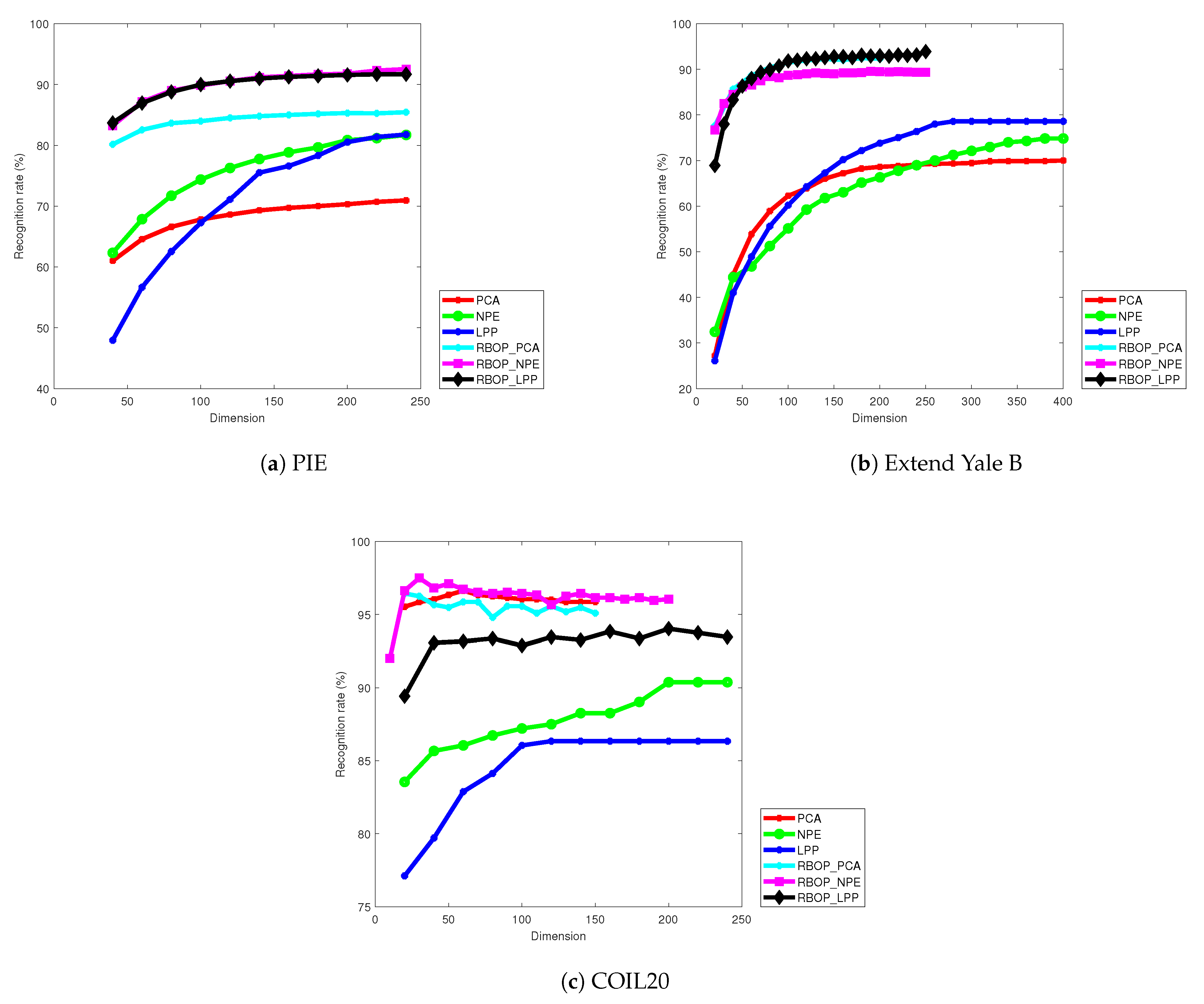
During the experimental phase, accurately presenting the experimental results of different methods under various dimensions is of crucial importance for algorithm evaluation and optimization. To this end, this paper selects three representative datasets, namely, PIE, Extended Yale B, and COIL20, to conduct experiments. The selection of samples strictly adheres to statistical norms. A total of 30 samples are randomly selected from each class in the PIE dataset, and 20 samples are randomly selected from each class in both the Extended Yale B and COIL20 datasets to form the training sample set, aiming to eliminate sample bias as much as possible.

Each group of experiments is run only once, with strict control over the consistency of conditions to reduce random errors. After completion, the focus is placed on the recognition accuracy rate and dimension changes, and the relationship between the two is precisely plotted in Figure 3. Here, the number of dimensions refers to the number of column vectors in the projection matrix P, which is related to dimensionality reduction and algorithm performance. By analyzing Figure 3, it can be seen that the RBOP_PCA, RBOP_NPE, and RBOP_LPP methods exhibit excellent performance in recognition accuracy on the three datasets. On the COIL20 dataset, the PCA method also achieves relatively good results. Based on the comprehensive experiment, the proposed methods can not only efficiently project the original images into low-dimensional subspaces and reduce the number of dimensions but also lead their counterparts in convergence speed, quickly approaching the global optimal solution. Through strict argumentation, the efficiency and scientific nature of the proposed methods have been verified, providing strong support for technological innovation in related fields.

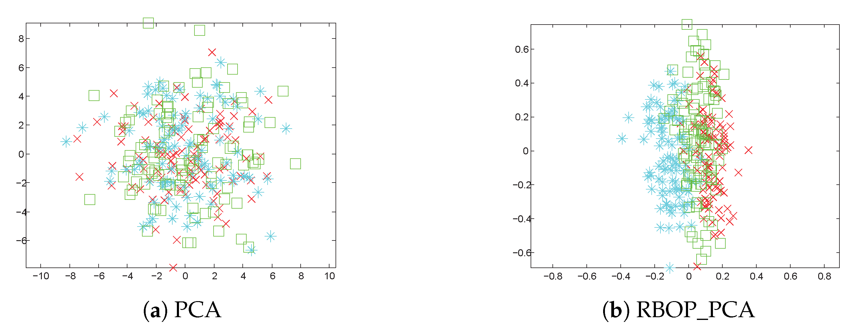
Subsequently, we showcase the results of applying various methods to three Gaussian synthetic datasets in Figure 4. Figure 4a,c,e display the classification outcomes utilizing PCA, NPE, and LPP. It is clear that these methods encounter difficulties in distinguishing between different objects (labeled as green squares, blue asterisks, and red crosses) based on the existing features. Figure 4b portrays the classification results of RBOP_PCA on the same dataset: blue asterisks, green squares, and red crosses are arranged sequentially along the horizontal axis from left to right. Figure 4d,f exhibit the classification results of RBOP_NPE and RBOP_LPP on the three Gaussian synthetic datasets. From this observation, we can identify three clear clusters, which further highlights that the performance of the proposed RBOP methods is superior to that of other traditional methods.

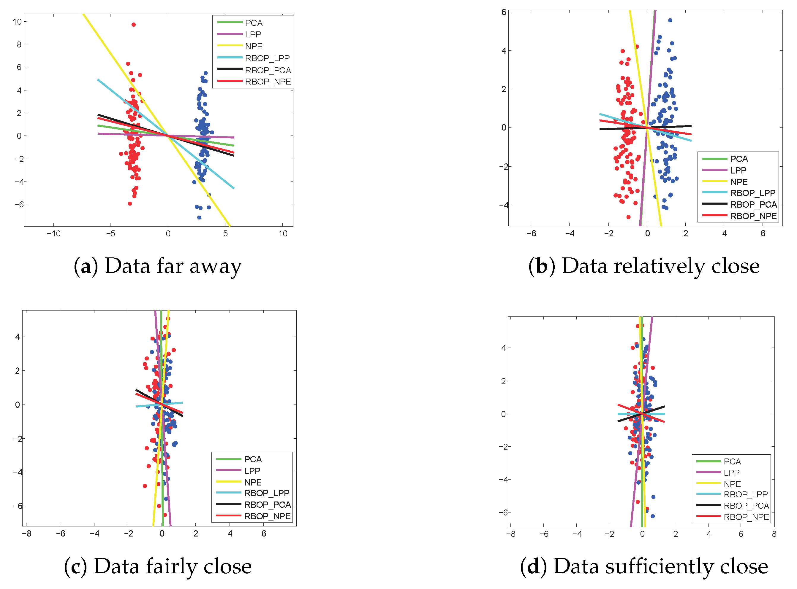
Finally, we illustrate the experimental outcomes of the two Gaussian synthetic datasets, as depicted in Figure 5. Distinct colored lines represent different methods. To categorize the data, denoted by red and dark blue dots, we project them vertically onto a straight line and subsequently differentiate the two clusters based on their projection position—theoretically, the greater the number of horizontal lines, the higher the classification accuracy. The observations from Figure 5a–d reveal that the proposed RBOP methods exhibit superior performance compared to traditional DR methods, particularly on data that are relatively, moderately, or sufficiently close.

5.4. Computational Efficiency Comparison

To showcase the computational efficiency of the proposed method, this subsection conducts a comparison of the runtime of this method with those of other benchmark methods. When setting up the experiment, a personal computer equipped with a 3.4 GHz central processing unit and 8 GB of memory serves as the hardware base. Windows 10 is chosen as the operating system, and Matlab 2015a is used to run all the methods. For simplicity and to focus on key data, the Extended Yale B dataset is selected for the experiment. By using a random sampling method, 30 images are randomly selected from the image set of each subject as training samples, so that the model can fully learn and extract key features. The remaining images are used as test samples to strictly verify the generalization performance and classification accuracy of the model. All data in each experiment link are collected and recorded meticulously. The key results are shown in

Table 6. Running time comparison among methods (seconds).

Algorithm	Training	Algorithm	Training	Algorithm	Training
PCA	0.03	NPE	0.12	LPP	0.14
RBOP_PCA	55.16	RBOP_NPE	71.34	RBOP_LPP	69.55

. It is found that the proposed methods take 55.16, 71.34, and 69.55 s, respectively, during different training rounds. As KNN is only used for image classification in the test set, and the running time of all methods is nearly the same in this regard, this part of the data is not recorded in detail. When making a horizontal comparison with classic methods like PCA, NPE, and LPP, the training time required by the proposed method is longer. However, it can achieve optimal classification results within about one minute. Therefore, in the pursuit of high-precision image classification, it is inevitable that a certain amount of computing time will be sacrificed. The proposed method has found a good balance, providing valuable reference for the design and improvement of similar algorithms.

6. Conclusions

This research presents a new robust bi-orthogonal projection framework called RBOP, which is based on projection learning, and provides a convergence analysis. We expand upon conventional DR methods (namely, PCA, NPE, and LPP) to develop RBOP (i.e., RBOP_PCA, RBOP_NPE, and RBOP_LPP). Under certain specific circumstances, the RBOP framework can revert to either PCA, NPE, or LPP. The RBOP methods demonstrate increased flexibility and robustness in comparison to traditional DR methods. RBOP integrates two orthogonal projections known as the “true” projection and “counterfeit” projection, enabling the learned optimal true projection to transform data more accurately during subspace learning. Through sparse reconstruction, this “true” projection can preserve the sparsity of the data in the original space from the low-dimensional subspace. Furthermore, by employing two different data reconstruction methods, the two projections can maintain the similar structure of the data.

Furthermore, by employing the sparse term to constrain noise, the RBOP method can effectively mitigate the impact of noise during the dimensionality reduction process. Computational experiments affirm the feasibility and effectiveness of the proposed methodology. Moreover, when applied to existing DR methods, it leads to enhanced precision and surpasses the performance of all other benchmark algorithms. Building upon the suggested framework, subsequent studies can improve both unsupervised and supervised techniques for tackling dimensionality catastrophes by expanding the RBOP methodology.