Design Oriented Analysis of Overhead Line Magnetic Energy Harvesters with Passive and Active Rectifiers

Abstract

The restructuring of the power grid calls for various energy harvesting technologies to power prospective remote electronic sensors, data loggers, and communication devices that could be installed at locations with restricted access. Magnetic energy harvesting stands out as a promising technology that is well suited for such applications while also being able to provide a significant amount of power. In this paper, a clamped-type overhead line magnetic energy harvester in configuration with passive and active rectifiers loaded with a constant voltage load is investigated. Here, an approximate piecewise linear model of the magnetic core is applied to represent the operation of the joint harvester–rectifier system. The main findings of this study include design-oriented analysis that easily lends itself to engineering applications. Based on the proposed analytical results, design guidelines are suggested to establish the key parameters of the harvester’s magnetic structure such as core size and number of secondary turns. Design examples are presented and verified using both simulation and experimental results. A good agreement of the results was found. The offered approach is simple and suitable for engineering purposes.

1. Introduction

Energy harvesting is about capturing stray or environmental energy and converting it to DC power that can be used to feed an electronic device. Maintenance-free harvesters present an attractive solution to powering equipment installed in hardly accessible locations.

Magnetic energy harvesters (MEH) rely on the magnetic field generated by current-carrying conductors of transmission lines or power transformers. Several types of MEHs were developed [1] that exploit different physical principles of interaction with the magnetic field such as variable reluctance [2,3], magnetostrictive [4,5], and ferrofluid [6,7,8] generators. The magnetic field generated by the line current can also be converted into the mechanical vibration of a miniature resonant cantilever. The output power can then be obtained by using a piezoelectric [9,10] or inductive [11] transducer mounted on the free end of the cantilever beam.

The concept of the clamped-on overhead line magnetic energy harvester (OLMEH) is illustrated in Figure 1 and can be found in earlier literature [12]. The advantage of the clamped-on magnetic harvester is that it can provide greater power density than the stick-on type of magnetic harvester [13] and a far greater power density than an electric field harvester [14]. Moreover, in comparison to solar power [15], a sensor fed by OLMEH is independent of environmental conditions and has no moving parts like the wind power generator [16]. Moreover, OLMEH is a quite robust and reliable device that requires no maintenance and can endure extreme weather conditions and, thus, is suitable to be installed in prohibitive locations. For these reasons, the clamp-on type OLMEH is a dependable prospective technology to implement a power supply unit for the new generation of smart wireless sensors, monitoring, surveillance, and communication equipment on high-voltage transmission lines and power plants [17].

The construction of OLMEH is quite similar to that of a current transformer (CT). CT, however, is a measurement device required to attain a highly accurate and linear relationship between the line current and the measured secondary current. Therefore, CTs are operated with short-circuited secondary winding. Thus, the magnetic operation point is established at the origin of the BH curve. However, the operating conditions of OLMEH are quite different. To extract the required power, OLMEH’s power processing circuit has to apply the battery voltage across OLMEH winding for a substantial time interval. This drives the magnetic core into saturation for a considerable portion of a line cycle. Meanwhile saturated OLMEH can provide no output current. Thus, to harvest any substantial power, OLMEH’s core material, geometry, and number of turns have to be properly selected. However, accurate OLMEH analysis is a challenging task due to the combined non-linearity of the magnetic core and the power processing circuit.

The complexity of OLMEH operation poses the problem of harvester design. To simplify matters, a piecewise linear approximation is adopted in this paper. As mentioned, OLMEH configurations with passive and active rectifiers were considered. The key contribution of this research encompasses a design-oriented analysis that readily adapts to engineering uses. Utilizing the suggested analytical results, design recommendations are proposed to determine the essential parameters of the harvester’s magnetic structure, such as magnetic core dimensions and the quantity of secondary windings.

Furthermore, the recent literature shows that to optimize the performance, OLMEH design should be properly matched to the load or provided with a maximum power point tracker [18,19,20]. The latter approach can suit only the active rectification scheme, which is more costly, but allows the extraction of higher power under variable parameters and operational conditions.

The rest of the paper is organized as follows: Section 2.1 presents the design-oriented analysis and guidelines of OLMEH with a passive rectifier. Section 2.2 offers the design-oriented analysis and guidelines of OLMEH with an active rectifier. Design examples are given in Section 2.3, followed by the experimental verification presented in Section 3. Finally, conclusions are given.

2. Methodology

This article presents a design-oriented analysis of a clamp-on type overhead line magnetic energy harvester with passive and active rectifiers feeding a constant voltage load (CVL). First, the model of the system is developed, then design guidelines and rules to help determine the magnetic parameters of the OLMEH are derived. The proposed approach provides meaningful analytical results suitable for engineering applications and is well supported by simulation and experimental results.

2.1. OLMEH with Passive Rectifier

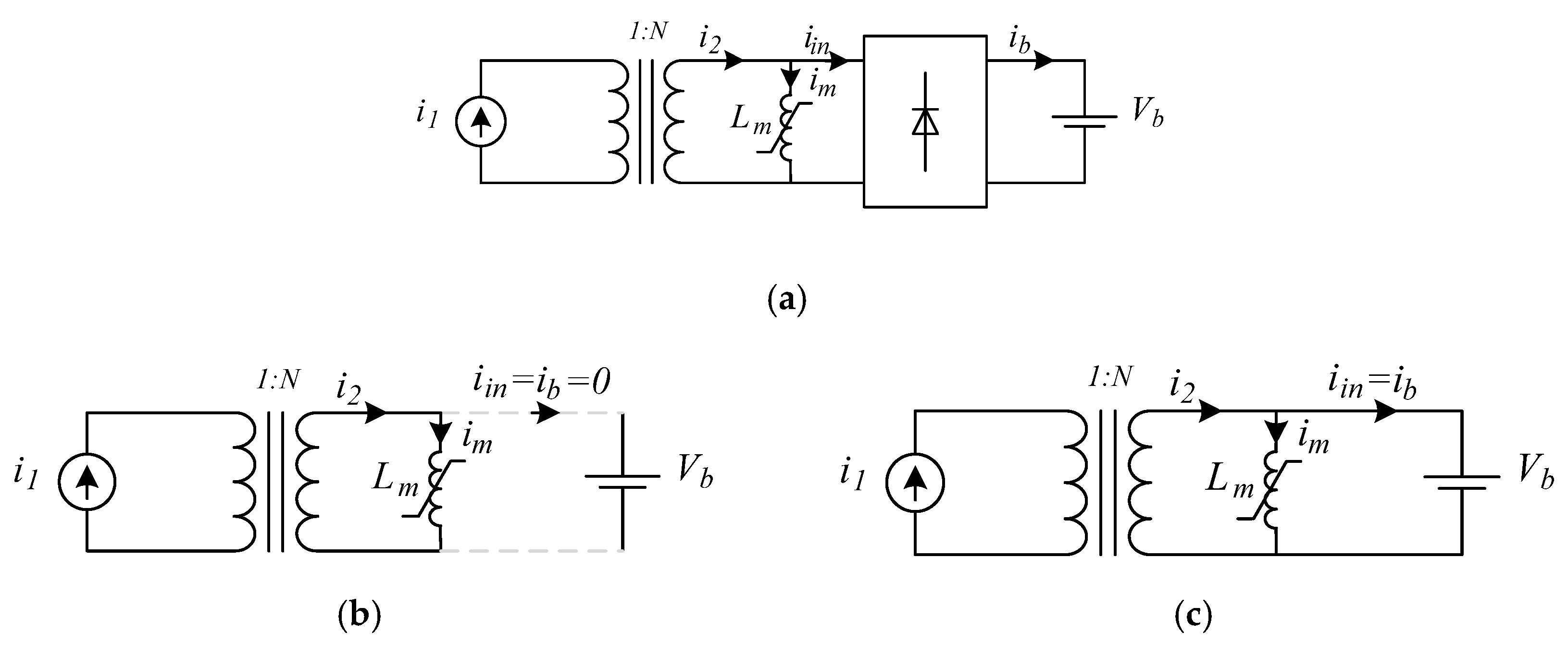
2.1.1. Basic Assumptions and Equivalent Circuits

OLMEH with a passive full-wave bridge rectifier providing DC power for a CVL load is illustrated in Figure 1. To facilitate the analysis approach, the following simplifying assumptions are adopted:

(a)

The hysteresis of the core material is neglected.

(b)

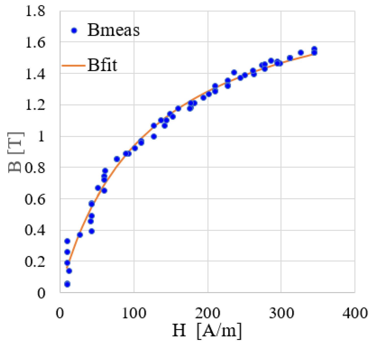
The core BH characteristic is approximated by a piecewise linear function.

(c)

A simplified cantilever model is used to represent the OLMEH magnetic circuit with the saturable magnetizing inductance, L_m, placed on the secondary winding, whereas the leakage inductance is neglected.

(d)

Lossless rectifiers are assumed.

The assumptions above lead to the OLMEH’s non-linear model illustrated in Figure 2a. Also shown are the equivalent circuits for the rectifier OFF and rectifier ON states; see Figure 2b and Figure 2c, respectively.

2.1.2. State Analysis of OLMEH with a Passive Rectifier

Examination of the simulation waveforms in Figure 3 reveals that the rectifier’s input current vanishes in a certain interval. As a result, two distinct time subintervals designated as State 1 and State 2 occur. The charging current only exists during State 2. Therefore, this operational mode is referred to as the discontinuous current mode (DCM).

The continuous current mode (CCM) prevails under low voltage conditions; however, it is of no interest in this paper because of its lower power yield.

State 1 commences with the magnetic core in deep saturation; see Figure 3. The voltage induced in the winding, $v_{in}$, is insufficient to turn on the rectifiers, and, therefore, the rectifier’s input current is zero, see the equivalent circuit in Figure 2b. The line current swings the magnetic field, H, and the magnetic flux density, B, so that the core is taken out of deep negative saturation towards a shallower saturation. As the magnetic flux density passes through the saturation knee and back to the linear region, the voltage induced in the OLMEH’s winding builds up; see Figure 3. When the induced voltage equals the CVL voltage, the rectifiers turn on. The secondary current, $i_2$, zero crossing is designated as the time reference $t=0$. Note that the rectifier’s turn-on instant, $t_1$, occurs before the start of the cycle, thus, $t_1<0$. The considerations above also suggest that at this instant, the flux density approximately equals the saturation knee flux density:

$$B_1\left(t_1\right)\approx -k_s{B}_s.$$

(1)

Here, $B_s$ is the core’s saturation flux density, and $k_s$ is an empirical saturation depth coefficient. A simulation study suggests that ${0.8<k}_s<0.9$.

State 2 commences at $t_1$. Here, the rectifier conducts while imposing a constant voltage of CVL across the harvester’s secondary; see the equivalent circuit in Figure 2c. As a result, the magnetic flux density in the core increases linearly with time (see Figure 3), thus:

$$B\left(t\right)={\displaystyle \frac{1}{N{A}_c}}{\int }_{t_1}^t{V}_{b}dt-k_s{B}_s={\displaystyle \frac{V_b}{N{A}_c}}\left(t-t_1\right)-k_s{B}_s,$$

(2)

Here, $N$ is the number of secondary turns, $A_c$ is the core cross-section, and $V_b$ is the CVL’s voltage.

State 2 terminates at $t_2$ when the flux density tends towards ${B\left(t_2\right)\approx k_{s}B}_s$. Therefore, from (2) the power transfer window is:

$$\left(t_2-t_1\right)=2k_s{\displaystyle \frac{N{A}_c{B}_s}{V_b }}.$$

(3)

The charge, $q$, delivered to the CVL during half the line cycle is:

$$q={\int }_{t_1}^{t_2}\left(i_2\left(t\right)-i_m\left(t\right)\right)dt,$$

(4)

Examining the simulation waveforms in Figure 3 suggests that $t_2\gg t_1$, therefore, $t_1$ can be neglected. Also, since the magnetizing current is quite small relative to the secondary current, $i_2\left(t\right)\gg i_m\left(t\right)$, and also having both positive and negative charge contributions that somewhat compensate each other (see Figure 3) (4) can be approximated by:

$$q\approx {\int }_0^{t_2}{i}_2\left(t\right)dt={\displaystyle \frac{I_{2m}}{\omega }}\left(1-\mathrm{c}\mathrm{os}\omega t_2\right),$$

(5)

Here, as usual, $\omega$ is line angular frequency and $f=\omega /2\pi$ is the line frequency.

Thus, the OLMEH’s average output power delivered to the CVL during the entire line cycle can be found by:

$$P_o=2fq{V}_b\approx {\displaystyle \frac{1}{\pi }}\left(1-\cos \omega t_2\right)V_b{I}_{2m}={\displaystyle \frac{\sqrt{2}}{\pi }}{\displaystyle \frac{1}{N}}\left(1-\cos \left(2k_s{\displaystyle \frac{\omega N{A}_c{B}_s}{V_b }}\right)\right)V_b{I}_{1rms},$$

(6)

Here, (3) was used (under the assumption $t_1=0$ stated above).

The expression for the charging power (6) can be rewritten as

$$P_o=\omega A_c{B_{s}F}_p\left({k_s,V}_N\right)I_{1rms},$$

(7)

where the power transfer function is defined as

$$F_p\left({k_s,V}_N\right)={\displaystyle \frac{\sqrt{2}}{{\pi }^2}}{V}_N\left(1-\cos \left(2k_s{\displaystyle \frac{\pi }{V_N}}\right)\right),$$

(8)

and the normalized CVL voltage is defined as

$$V_N={\displaystyle \frac{\pi }{\omega }}{\displaystyle \frac{V_b}{N{A}_c{B}_s}},$$

(9)

The normalized variable $V_N$ has a physical meaning as a ratio of the maximum available volt∙sec that can be delivered to the core during one half-cycle of the line, ${\displaystyle \frac{\pi }{\omega }}{V}_b$, to the theoretical maximum flux linkage of the core, $N{A}_c{B}_s$.

Examination of (8) suggests that for low values of the variable $V_N$, the power transfer function, $F_p\left(k_s,V_N\right)$, is rapidly oscillating and has an infinite number of local extremum points. However, the power transfer function has a global maximum and for an assumed value of $k_s=0.83$ attains the peak value of $F_p\left(\mathrm{0.83,2.03}\right)=0.49$, at $V_{N mpp}=2.03$; see Figure 4.

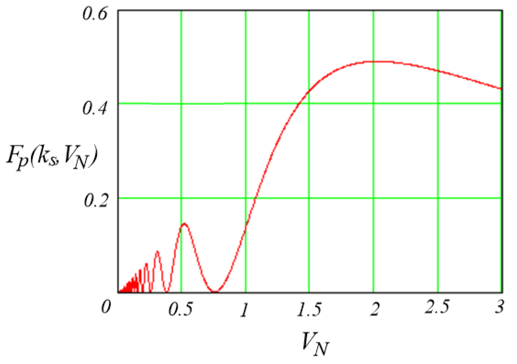
2.1.3. Design Guidelines of an OLMEH with a Passive Rectifier

The following design guidelines show how to establish the required core cross-sectional area, $A_c$, and the required number of turns of the secondary winding N, so that the designed OLMEH can provide the required output power $P_o$ for the line current of $I_{1rms}$. The angular frequency of the line, $\omega$, is assumed to be known.

The design starts with choosing a low-loss magnetic core material with a soft BH curve having a high saturation flux density.

The next step is extracting the material’s parameter $B_s$.

The minimum required core cross-section can be established by plugging the mentioned peak value of the power transfer function, $F_p\left(\mathrm{0.83,2.03}\right)=0.49$, into (7):

$$A_{cmin}\approx {\displaystyle \frac{P_{omin}}{0.49\omega B_s{I}_{1rms min}}},$$

(10)

Chose a suitable core with $A_c>A_{cmin}$. Also, consider that the core has to accommodate a rather thick primary conductor (cable). A “sausage” (a small diameter tube) core shape is most suitable for OLMEH design. Such a core shape can provide the required cross-section area at minimum magnetic path length, thus minimizing OLMEH’s volume and weight.

Calculate the required number of turns from (9), while plugging the value for the normalized MPP voltage, $V_{N mpp}=2.03$, and considering the rectifier’s voltage drop, $V_D\approx 1.5 V$, that is using ${V^{\prime }}_b=V_b+2V_D.$

$$N={\displaystyle \frac{\pi }{\omega }}{\displaystyle \frac{V_b+2V_D}{V_N{A}_c{B}_s}},$$

(11)

The average diode current can be found from (6) as

$$I_{Dav}\approx {\displaystyle \frac{1}{\sqrt{2}\pi }}{\displaystyle \frac{I_{1rms}}{N}}\left(1-\cos \omega t_2\right),$$

(12)

whereas the rms diode current can be approximated by

$$I_{Drms}\approx {\displaystyle \frac{I_{1rms}}{N}}\sqrt{{\displaystyle \frac{1}{\pi }}\left(2\omega t_2-\sin 2\omega t_2\right)},$$

(13)

where $t_2$ is given by (3) (recall that $t_1=0$ is assumed).

In case the design does not attain the desired power, the initial guess of $k_s=0.83$ (here, obtained from simulation) should be revised. To improve the design, use the measured results to recalculate $k_s$ from Equation (6) and iterate.

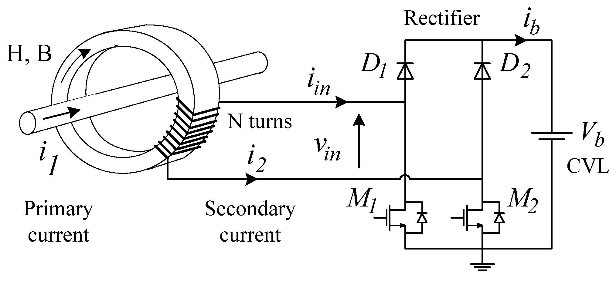
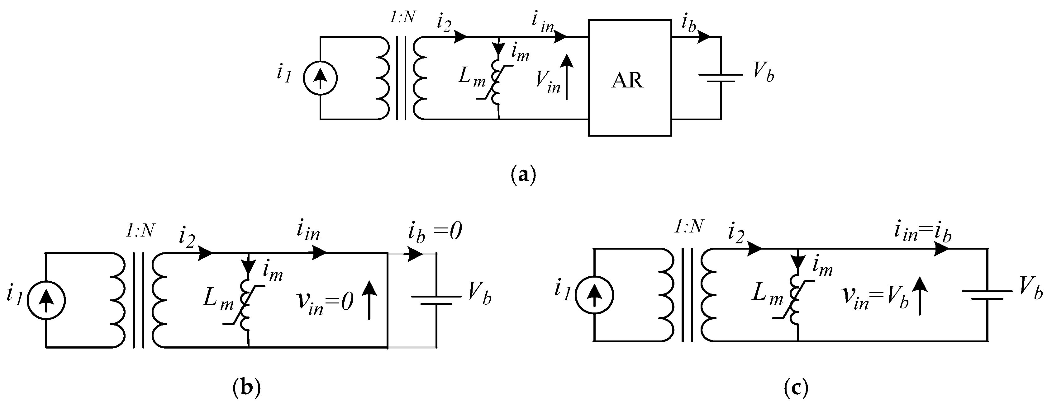
2.2. OLMEH with Active Rectifier

Several topologies of active rectifiers are known. Here, OLMEH with an Active Rectifier (AR) in the push-pull configuration, shown in Figure 5, is considered. There are two major differences between the operation of OLMEH with a passive rectifier described above and the active rectifier case, described below. Firstly, with an active rectifier, the controller can command to short the OLMEH’s secondary winding and so preserve the magnetic energy in the core. Secondly, the controller can initiate rectifier conduction at an optimal delay time, $t_1$, to allow a higher current for the load but also release the energy stored in the core towards the load. These features allow OLMEH with the active rectifier to develop a higher power than with a passive rectifier configuration.

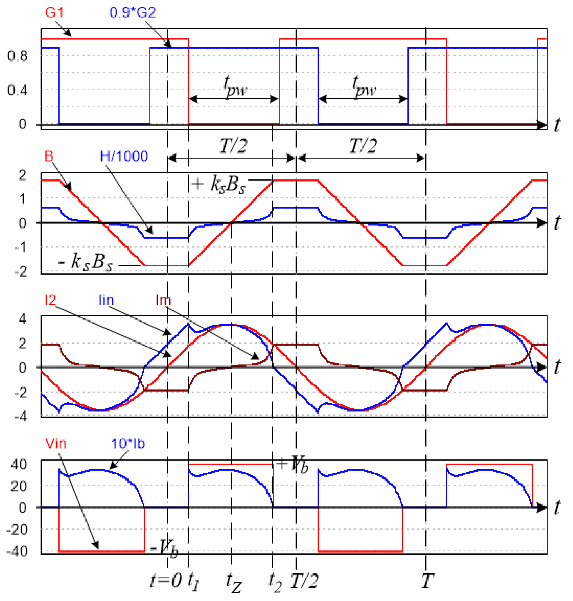
2.2.1. State Analysis of OLMEH with Active Rectifier

Due to the half-wave symmetry of OLMEH’s operation (see the simulated waveforms in Figure 6) it is sufficient to describe only the positive half cycle (i.e., for the positive secondary current, $i_2\left(t\right)>0$).

The analysis is based on the above assumptions (a)–(d) regarding the properties of the magnetic core, (see Section 2.1.1). These lead to the OLMEH’s non-linear model, illustrated in Figure 7a.

State 1 $\left[0, t_1\right]$ (see Figure 7b) commences at $t=0$. Here, both active switches conduct and short the secondary winding. As a result, the flux density, B, the field intensity, H, and the magnetizing current, im, in the core remain constant, whereas the rectified current is zero, ib = 0.

State 2 $\left[t_1, t_2\right]$ (see Figure 7c) commences at $t=t_1$, when, by controller’s command, the M1 switch is turned off but M2 remains on. Here, the rectifier diode D1 turns on and allows charging current to the CVL. Since the rectifier applies a constant voltage of the CVL to the secondary winding, the flux density in the core starts ramping up linearly. (In practice, the field intensity, H, and the magnetizing current, $i_m$, rise in a non-linear fashion as shown in Figure 6).

State 2 terminates as the magnetizing current equals the secondary current, and the rectifiers’ current ceases at a certain instant, $t_2$: $i_2\left(t_2\right)=i_m\left(t_2\right)\Rightarrow i_b\left(t_2\right)=0$. Here, the controller turns on the M1 switch to short-circuit the OLMEH’s winding.

During $\left[t_2, T/2\right]$, both the rectifier switches M1 and M2 conduct and keep the OLMEH winding shorted. Thus, OLMEH is reverted to State 1 until the end of the half cycle.

A similar order of events occurs during the negative half-cycle with M2 interchanging its function with M1 while D2 interchanges its function with D1.

CVL takes current during State 2, which, as mentioned, commences at $t_1$ and terminates at $t_2$; see Figure 6. The constant voltage, across the harvester’s secondary winding (see Figure 7c), results in a linear increase in the magnetic flux density from the initial value of $-k_s{B}_s$ towards the final value $k_s{B}_s$. Therefore, the power transfer window width is the same as (3). However, in OLMEH AR case, $t_1$ is determined by the controller’s command.

The input current of the rectifier is the difference between the secondary current, $i_2\left(t\right)$, and the magnetizing current, $i_m\left(t\right)$. Therefore, the charge delivered to the CVL during the half cycle is similar to (4), yet considering, $t_1$:

$$q_b={\int }_{t_1}^{t_2}\left(i_2\left(t\right)-i_m\left(t\right)\right)dt,$$

(14)

Examining the steady-state waveforms in Figure 6 reveals that the magnetizing current is perfectly symmetrical. This suggests that the net charge contributed by the magnetizing current is zero:

$${\int }_{t_1}^{t_2}{i}_m\left(t\right)dt=0,$$

(15)

This also complies with the conservative nature of the magnetizing inductance that, under the assumption of a lossless circuit, completely recycles the stored energy.

Combining (14) and (15) yields the charge delivered to the CVL:

$$q_b={\int }_{t_1}^{t_2}{I}_{2m}\sin \left(\omega t\right)dt={\displaystyle \frac{I_{2m}}{\omega }}\left(\cos \left(\omega t_1\right)-\cos \left(\omega t_2\right)\right),$$

(16)

whence the OLMEH’s average output power can be found:

$$P_o=2f{q}_b{V}_b={\displaystyle \frac{\sqrt{2}}{\pi N}}{V}_b{I}_{1rms}\left(\cos \left(\omega t_1\right)-\cos \left(\omega t_2\right)\right),$$

(17)

The OLMEH’s power output can be optimized when the power transfer window is aligned symmetrically to the line current peak, see Figure 6, that is

$$t_{2_{opt}}={\displaystyle \frac{T}{2}}-t_{1opt},$$

(18)

Substituting the optimum condition (18) into (17) gives:

$$P_{opt}={\displaystyle \frac{2\sqrt{2}}{\pi N}}{V}_b{I}_{1rms}\mathit{cos}\left(\omega t_{1opt}\right),$$

(19)

The optimal delay time can be expressed by applying (3) to (18) as:

$$t_{1opt}={\displaystyle \frac{T}{4}}-{\displaystyle \frac{\left(t_{2opt}-t_{1opt}\right)}{2}}={\displaystyle \frac{T}{4}}-k_s{\displaystyle \frac{N{A}_c{B}_s}{V_b }},$$

(20)

This can be written in the normalized form as

$$t_{1optN}={\displaystyle \frac{t_{1opt}}{T/2}}={\displaystyle \frac{1}{2}}-k_s{\displaystyle \frac{1}{V_N }},$$

(21)

where $V_N$ is the normalized CVL voltage as defined in (9). Note that the lower limit of the normalized CVL voltage, which still preserves the desired operational mode, can be found by substituting $t_{1optN}=0$ into (21) yielding $V_{Nmin}=1.667$. Higher values of the CVL voltage reduce the pulse width of the charging current and thus, increase the delay time.

Substituting (20) into (19) yields the optimum/maximum available power:

$$P_{opt}={\displaystyle \frac{2\sqrt{2}}{\pi N}}{V}_b{I}_{1rms}\mathit{sin}\left(k_s{\displaystyle \frac{\omega N{A}_c{B}_s}{V_b }}\right),$$

(22)

Furthermore, (22) can be rewritten as:

$$P_{opt}=\omega A_c{B}_s{F}_a\left(k_s,V_N\right)I_{1rms},$$

(23)

where the power transfer function of OLMEH with an active rectifier is defined as

$$F_a\left(k_s,V_N\right)={\displaystyle \frac{2\sqrt{2}}{{\pi }^2}}{V}_{N}sin\left(k_s{\displaystyle \frac{\pi }{V_N}}\right),$$

(24)

The power transfer function $F_a\left(k_s,V_N\right)$ is a convex function of the normalized CVL voltage, $V_N$; see Figure 8. Evidently, in the range $1.667<V_N<5$ increasing the volt per turn, i.e., decreasing the number of turns (see (9)) helps to extract higher power from OLMEH, yet the function reaches an upper limit of $F_a\left(k_s,V_N\right)\underset{V_N\to \infty }{\to }0.75$ (for $k_s=0.83$).

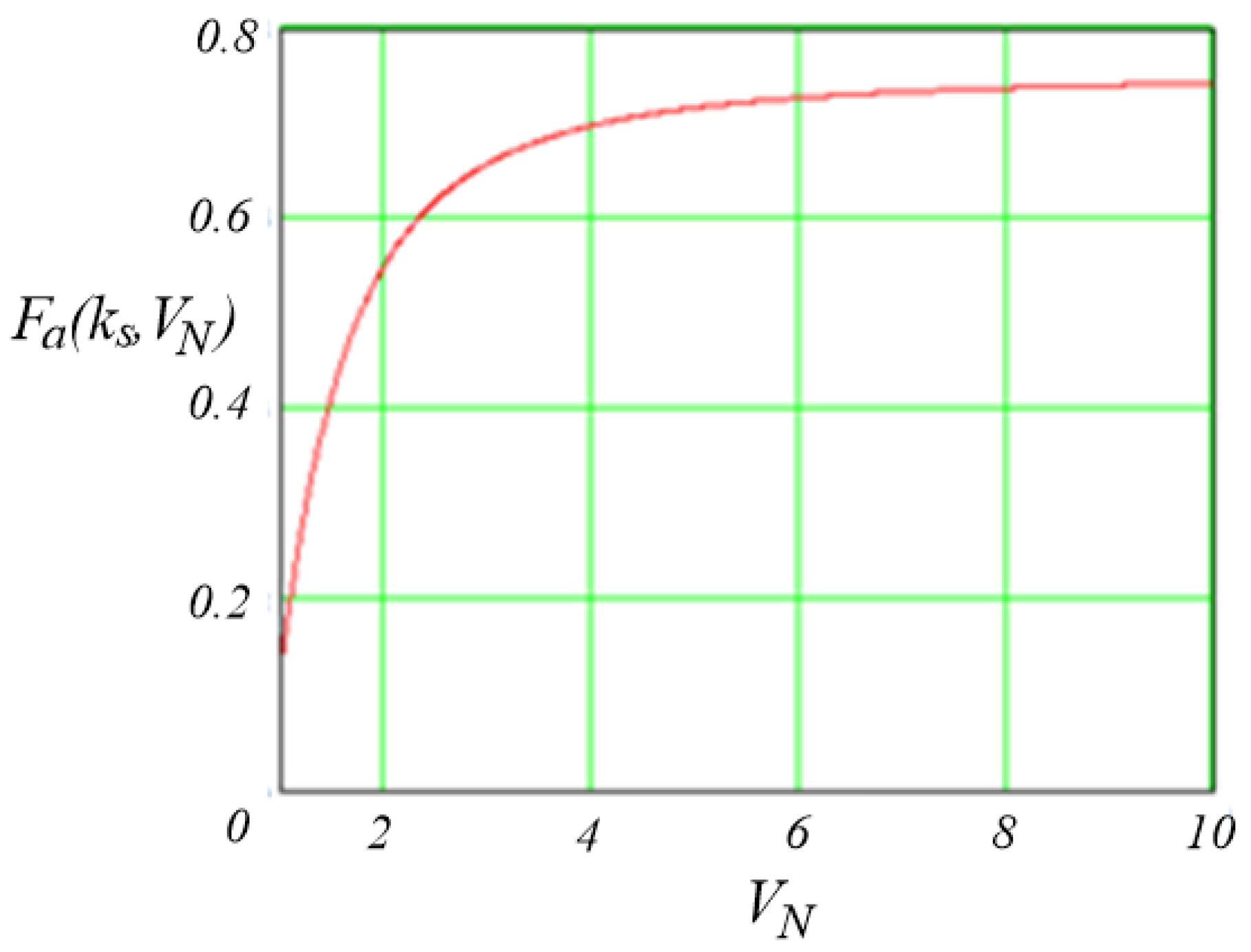
2.2.2. Design Guidelines for OLMEH with an Active Rectifier

The following design guidelines show how to establish the required delay time, $t_1$, the core cross-sectional area, $A_c$, and the required number of turns of the secondary winding N, so that the designed OLMEH can provide the required output power $P_{opt}$ into a constant voltage load, $V_b$, at line condition, $I_{1rms}$. The angular frequency of the line, $\omega$, is assumed to be known.

The design starts with choosing a magnetic material and finding its saturation flux density, $B_s$.

This design guideline suggests setting the delay time to:

$$t_{1opt}={\displaystyle \frac{\pi /6}{\omega }},$$

(25)

so as to eliminate the triple harmonics of the voltage applied to the OLMEH’s winding and decrease the core losses.

Combine (25) and (21) to find the normalized load voltage:

$$V_N=2k_s{\displaystyle \frac{\pi }{\left(\pi -2\omega t_{1opt}\right)}},$$

(26)

For the initial guess of $k_s$, and plugging the result of (26) into (24) gives the value of the power transfer function, $F_a\left(k_s,V_N\right)$.

Then, the minimum required core cross-section can be established from (23).

$$A_{cmin}\approx {\displaystyle \frac{P_{opt}}{F_a\left(k_s,V_N\right)\omega B_s{I}_{1rms}}},$$

(27)

Chose a suitable core with $A_c>A_{cmin}$. Again, consider that the core window has to accommodate a rather thick primary conductor (cable). As suggested above, a “sausage”- shaped core is preferred.

Calculate the required number of turns from (14), while plugging the value for the normalized CVL voltage, (30), and considering the rectifier’s voltage drop, $V_D$.

$$N\approx {\displaystyle \frac{\pi }{\omega A_c{B}_s}}{\displaystyle \frac{V_b+2V_D}{V_N}},$$

(28)

The diode average current can be derived from (19):

$$I_{Dav}={\displaystyle \frac{\sqrt{2}}{\pi N}}{I}_{1rms}\mathit{cos}\left(\omega t_{1opt}\right),$$

(29)

the rms diode current can be approximated by

$$I_{Drms}\approx {\displaystyle \frac{I_{1rms}}{N}}\sqrt{{\displaystyle \frac{1}{2\pi }}\left(\pi -2\omega t_1+\sin 2\omega t_1\right)},$$

(30)

whereas MOSFET’s rms current can be approximated simply by

$$I_{Mrms}\approx {\displaystyle \frac{I_{1rms}}{N}},$$

(31)

Alternatively, a designer might want to consider the maximum allowable short-circuit current, $I_{b rms MAX}$, that flows through the semiconductor switches during continuous short-circuit conditions as an additional design constraint. In such a case, the design procedure unfolds as follows.

Start with choosing a magnetic material and finding its saturation flux density, $B_s$.

Since OLMEH’s core goes in and out of saturation, the output current, $I_{b rms}$, available for CVL is lesser than the value of the short-circuit secondary current, $I_{b rms MAX}$. Therefore, the number of turns, $N$, can be established according to:

$$N={\displaystyle \frac{I_{1rms}}{I_{b rms MAX}}},$$

(32)

which ensures that the rms secondary short-circuit current complies with the desired current limitation $I_{b rms}<I_{b rms MAX}$.

The minimum required core cross-section can then be established from (11), also considering diodes’ voltage drop

$$A_{cmin}={\displaystyle \frac{V_b+2V_D}{k_s\omega N{B}_s}}{\sin }^{-1}\left({\displaystyle \frac{\pi N}{2\sqrt{2}}}{\displaystyle \frac{P_{opt}}{V_b{I}_{1rms}}}\right),$$

(33)

Choose a suitable core with $A_c>A_{cmin}$ and sufficient window area.

Calculate the optimum delay time, $t_{1opt}$, according to (20).

Semiconductors’ currents can be estimated as suggested above; see (29)–(31).

2.3. Design Examples

2.3.1. Design Example 1: OLMEH with a Passive Rectifier

The following design example establishes the required core cross-sectional area, Ac, and the required number of turns, N, so that the designed OLMEH can provide the minimum required output power Pomin = 50 W into a $V_b=24 \mathrm{V}$ CVL, at the worth line condition, $I_{1 rms min}=100$ A rms. The angular frequency of the line is $\omega =314 \mathrm{rad}/\mathrm{s}$.

Choose a low-loss magnetic core material with a soft BH curve having a high saturation flux density. As an example, silicon steel from EILOR MAGNETIC CORES, Israel, was chosen.

The next step is extracting the material’s parameters. The experimentally measured BH data vs. the fitted BH curve is shown in Figure 9. Froelich approximation was used:

$$B\left(H\right)={\displaystyle \frac{aH}{b+\left|H\right|}},$$

(34)

Froelich parameter a represents the asymptotic value of the saturation flux density, B_s:

$$B_s=\underset{H\to \infty }{\lim }{\displaystyle \frac{aH}{b+H}}=a,$$

(35)

Here, $B_s=a=2.05$ and $b=109.4$ were found by curve fitting; see Figure 9.

Find the minimum required core cross-section by plugging the initial guess of $k_s=0.83$, and the maximum value of the power transfer function, $F_p\left(0.83, 2.03\right)=0.49$, into (27):

$$A_{cmin}={\displaystyle \frac{50}{0.49·314·2.05·100}}=1624·{10}^{-6},$$

(36)

Thus, the OLMEH’s core should have $A_c>A_{cmin}$, for instance $A_c=1800$ mm².

Find the required number of turns by plugging $V_{Nmpp}=2.03$ and the rectifier’s voltage drop, $V_D\approx 1.5 \mathrm{V}$, into (11):

$$N={\displaystyle \frac{\pi }{314·2.05·1800{·10}^{-6}}}{\displaystyle \frac{24+3}{2.03}}=36.9,$$

(37)

In practice, some adjustments can be expected.

2.3.2. Design Example 2: OLMEH with an Active Rectifier

The following design example establishes the required delay time, t1, the core cross-sectional area, $A_c$, and the required number of turns of the secondary winding N, so that the designed OLMEH can provide the minimum required output power Popt = 70 W into a $V_b=45$ V CVL, at line condition, $I_{1rms}=100$ A rms. The angular frequency of the line is $\omega =314 \mathrm{r}\mathrm{a}\mathrm{d}/\mathrm{s}$.

Similar to the example above, a silicon steel core from EILOR MAGNETIC CORES, Israel, was chosen.

Then, the core parameters are extracted as mentioned above. Here, $B_s=2.05$ [T] was found.

To minimize the harmonics of the voltage applied to the OLMEH’s winding set the delay time according to (25)

$$t_{1opt}={\displaystyle \frac{\pi /6}{\omega }}=1.67 [\mathrm{m}\mathrm{S}],$$

(38)

With the initial guess of $k_s=0.83$, the normalized load voltage is calculated according to (26):

$$V_N=2k_s{\displaystyle \frac{\pi }{\left(\pi -2\omega t_{1opt}\right)}}=2.5,$$

(39)

Find the value of the power transfer function (24), $F_a\left(0.83, 2.5\right)=0.62$. Then, substitute into (27) to establish the required core cross-section:

$$A_{cmin}={\displaystyle \frac{70}{0.62·314·2.05·100}}=1754·{10}^{-6},$$

(40)

Choose a suitable core with $A_c>A_{cmin}$; for instance with $A_c=1800$ mm².

Calculate the required number of turns from (28), plugging, $V_N=2.5$, and $V_D\approx 1.5 \mathrm{V}$:

$$N={\displaystyle \frac{\pi }{314·2.05·1800{·10}^{-6}}}{\displaystyle \frac{45+1.5}{2.5}}=50,$$

(41)

Simulated waveforms of the OLMEH AR design example are shown in Figure 10. The simulated design achieved 73 W of output power at line condition, $I_{1rms}=100$ A rms.

Note that according to the simulation results in Figure 10, the peak flux density is $k_s{B}_s$= 1.7. Using the obtained above estimation of the saturation flux density, $B_s$ = 2.05, suggests that $k_s=1.7/2.05=0.83$. This justifies the value of $k_s$ used for the design examples.

2.3.3. Design Example 3: OLMEH with an Active Rectifier

Let the design specifications be $P_o=75 \mathrm{W}$ of output power into a Vb = 45 V CVL, at line current, $I_{1rms}=100$ A rms, and introducing the limitation of maximum allowable short-circuit current $I_{b rms MAX}=2.5$ A rms at the angular frequency $\omega =314 {\displaystyle \frac{\mathrm{rad}}{\mathrm{S}}}$.

Start with choosing an appropriate soft magnetic material with high saturation flux density, $B_s$.

Then, the core parameters are extracted as described above yielding $B_s$ = 2.05.

Find the number of turns, N, according to (32):

$$N={\displaystyle \frac{I_{1rms}}{I_{b rms MAX}}}={\displaystyle \frac{100}{2.5}}=40,$$

(42)

The minimum required core cross-section can then be established from (22), also considering diodes’ voltage drop $V_D=1.5 \mathrm{V}$

$$A_{cmin}={\displaystyle \frac{V_b+V_D}{k_s\omega N{B}_s}}{\sin }^{-1}\left({\displaystyle \frac{\pi }{2\sqrt{2}}}{\displaystyle \frac{{NP}_{opt}}{V_b{I}_{1rms}}}\right)={\displaystyle \frac{45+1.5}{0.83·314·40·2.05}}{\sin }^{-1}\left({\displaystyle \frac{\pi }{2\sqrt{2}}}{\displaystyle \frac{40·75}{(45+1.5)·100}}\right)=1738·{10}^{-6}$$

(43)

A suitable core with $A_c>A_{cmin}$ can be same as above $A_c=1800{·10}^{-6}$.

Calculate the optimum delay time, $t_{1opt}$, according to, (20):

$$t_{1opt}={\displaystyle \frac{T}{4}}-k_s{\displaystyle \frac{N{A}_c{B}_s}{V_b }}=0.005-0.83{\displaystyle \frac{40·1800{·10}^{-6}·2.05}{45+1.5}}=2.36{·10}^{-3}$$

(44)

The semiconductors’ currents during normal operation can be estimated by (29)–(31).

Comparison of the simulation vs. the design goals and the calculated results is presented in

Table 1. Comparison of the calculated vs. the simulated results of Example 3.

Param. (eq.)	${\mathit{P}}_{\mathit{o}}$ (23)	${\mathit{I}}_{\mathit{D}\mathit{a}\mathit{v}}$ (29)	${\mathit{I}}_{\mathit{D}\mathit{r}\mathit{m}\mathit{s}}$ (30)	${\mathit{I}}_{\mathit{b}\mathit{r}\mathit{m}\mathit{s}}$
Calculated	75 (goal)	0.8	1.6	2.5 (goal)
Simulated	80	0.9	1.7	2.4

. A good match is found.

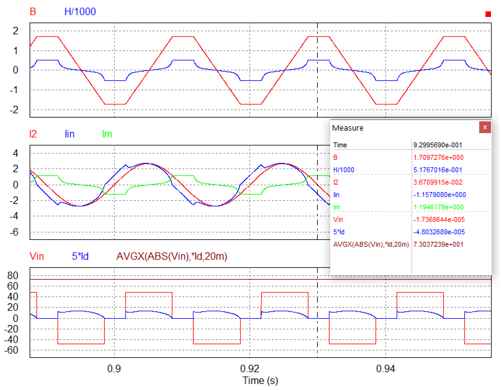
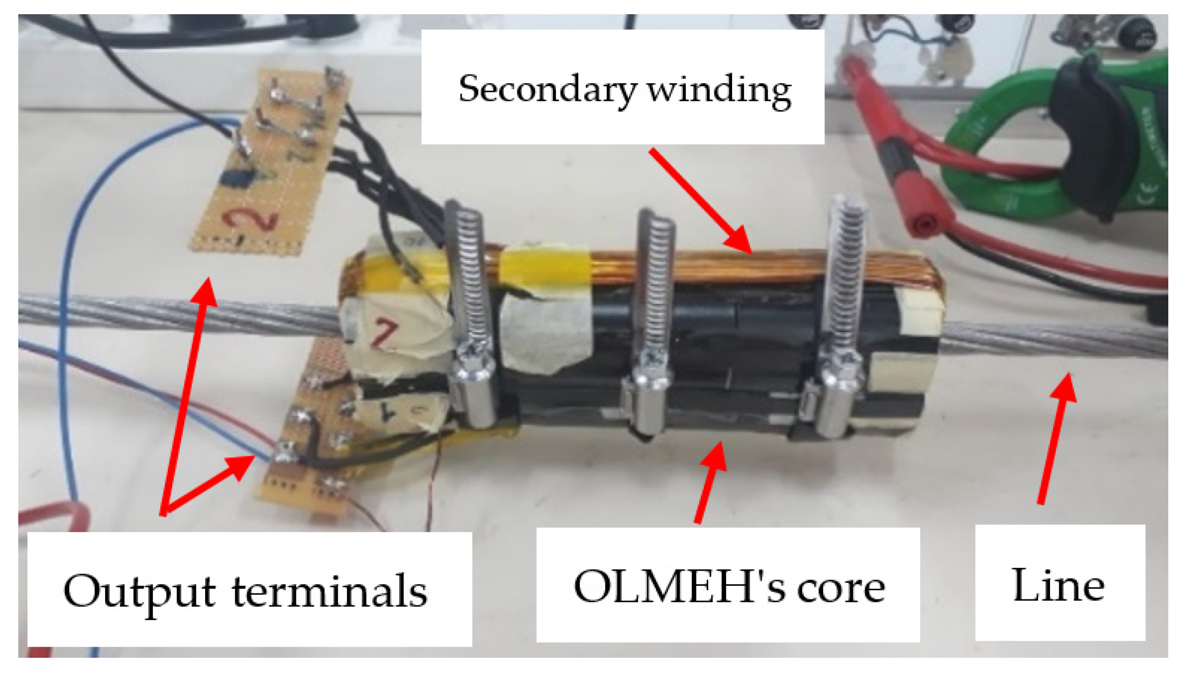
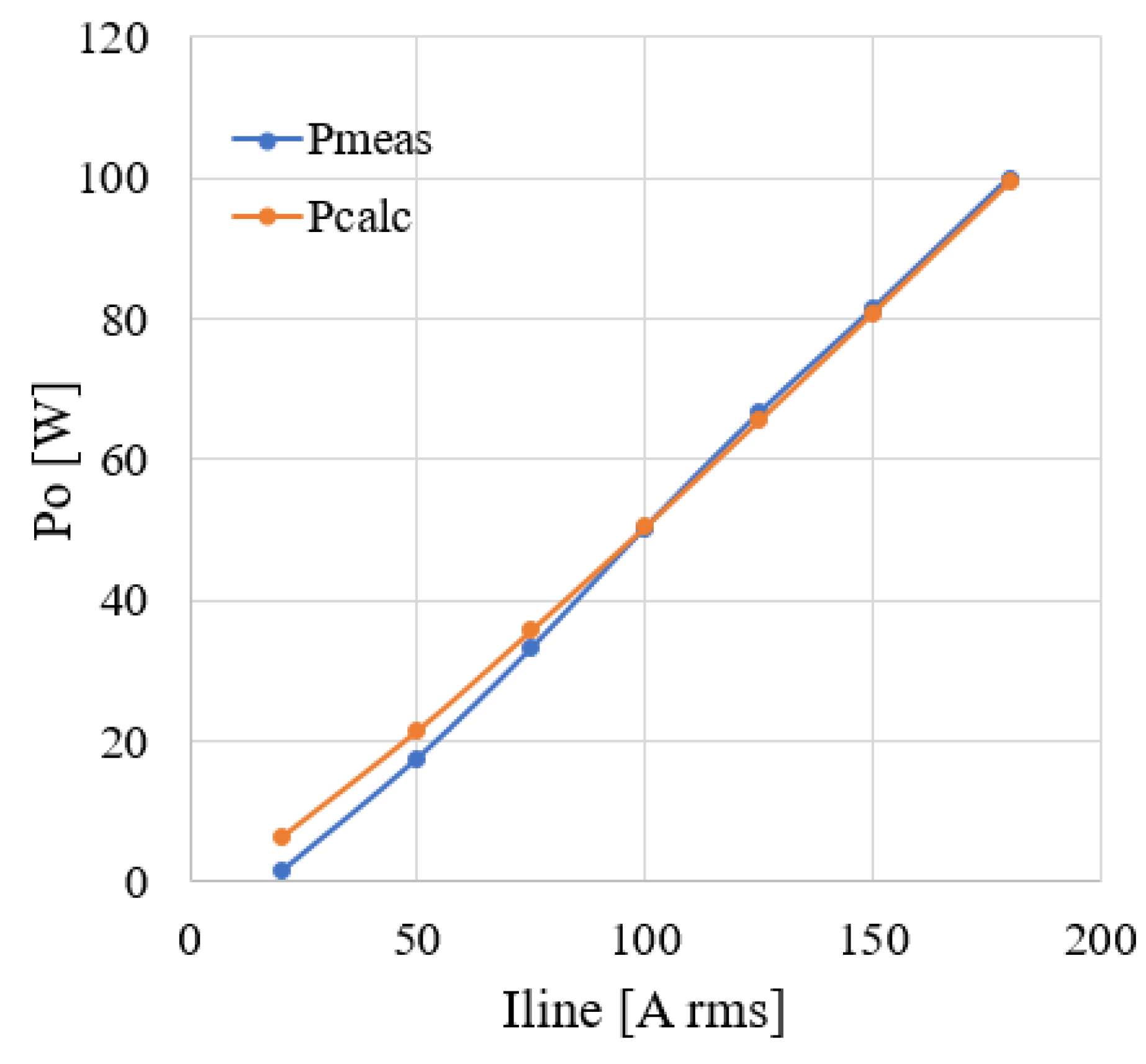
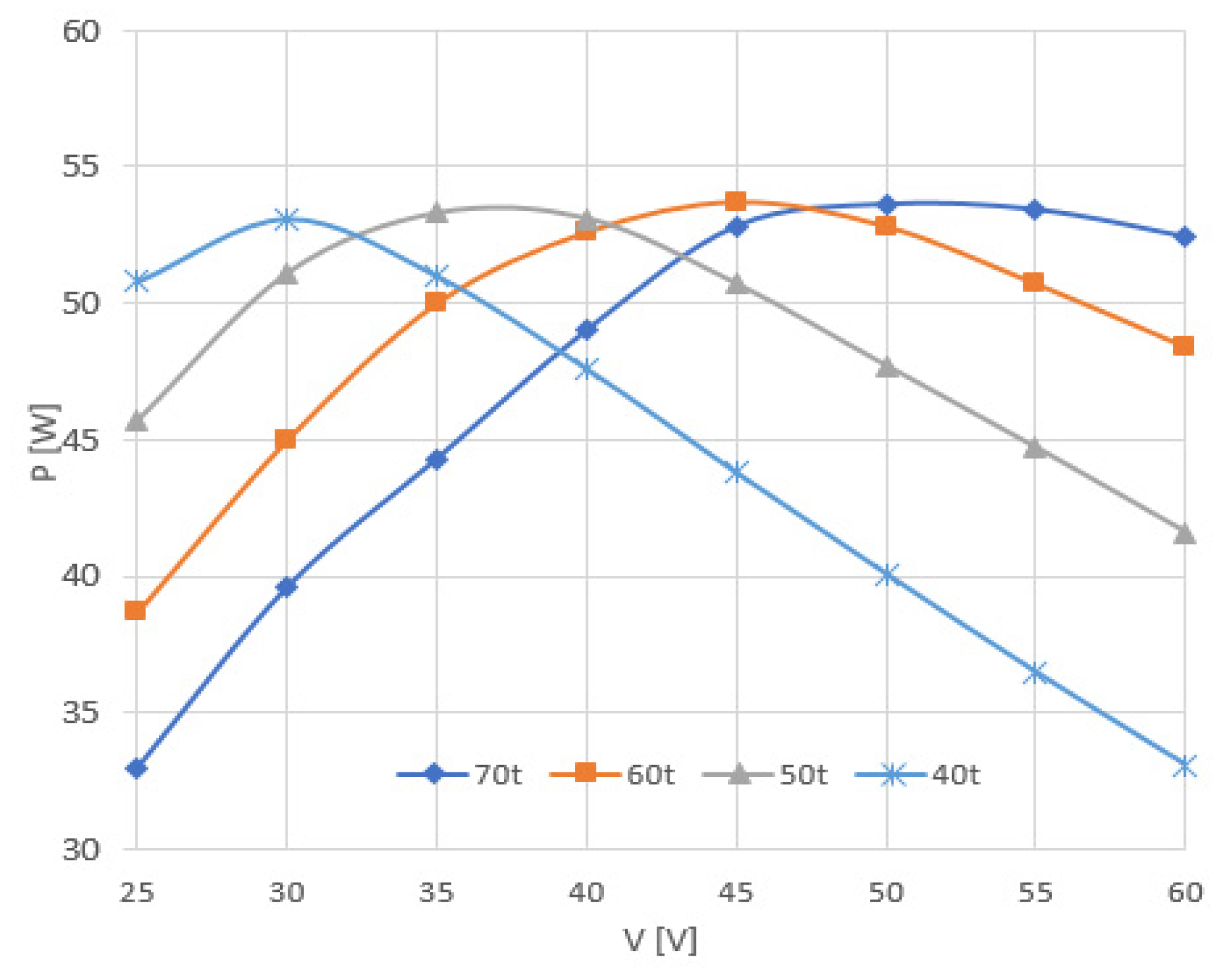
3. Validation and Experimental Results

An experimental laboratory prototype OLMEH was built and tested. The OLMEH’s core was constructed by stacking together three pairs of silicon steel 10 H10 C-cores with a total core cross-section of $A_c$= 1800 mm² and a magnetic path length of $l_c$ = 120 mm (EILOR MAGNETIC CORES, Israel). OLMEH windings were made reconfigurable and allowed for $N$ of 40, 50, 60, and 70 turns. A view of the prototype is shown in Figure 11.

To test the performance of the prototype OLMEH, an experimental test bed was constructed, capable of sustaining line current of up to 200 A rms. An electronic load was used to emulate the constant voltage sink load.

Key waveforms of the OLMEH in the DCM mode are shown in Figure 12.

A comparison of the calculated vs. the measured output power as a function of the line current at fixed battery voltage is presented in Figure 13 and supports the derived expression for OLMEH’s output power (6). Here, the OLMEH configuration was similar to the Design Example 1 and had a core cross-section of $A_c=1800$ mm², while the number of turns was rounded to $N=40$ t.

The OLMEH was also tested at different CVL voltage levels. The plot of OLMEH’s output power vs. the CVL voltage at a line current of 100 A rms is shown in Figure 14. The maximum output power predicted by (6) is Po = 56 W. The experimentally measured maximum power stood in good agreement with the theoretical prediction and was in the range of 53–54 W for all four windings configurations; see Figure 14.

As predicted, the maximum power point voltage as a function of the number of turns was calculated by (7) while substituting $V_{Nmpp}=$2.03 and considering the rectifier’s voltage drop of approximately ${2V}_D=3 \mathrm{V}$. A good match with the experimental results is found; see Figure 14 and

Table 2. Comparison of the calculated vs. the experimental MPP voltage as a function of the number of turns.

N [Turn]	40	50	60	70
$V_{bmpp}$ [V] predicted	26.9	34.3	41.8	49.2
$V_{bmpp}$ [V] experimental	30	37	45	51

.

A comparison plot of experimentally measured vs. the calculated by (22) OLMEH’s output power as a function of the delay time at a line current of $I_1=100 \mathrm{A} \mathrm{rms}$, under the constant voltage load, $V_b=45 \mathrm{V}$, is shown in Figure 15.

The experimental waveforms of OLMEH with an active rectifier in Figure 5 under CVL of $V_b=45 \mathrm{V}$ are shown in Figure 16. OLMEH had the same parameters as in Design Example 3 ($A_c=1800$ mm² and $N=40$ turns). The maximum output power predicted by the lossless model (22) was $P_o=76 \mathrm{W}$ and stood in good agreement with the experimentally measured $P_o=74 \mathrm{W}$.

4. Conclusions

This paper offers a design-oriented analysis for an overhead line magnetic energy harvester with either passive or active rectifiers under a constant voltage load. Based on the analytical considerations design guidelines for the mentioned type of energy harvesters were derived and design examples were offered.

The laboratory prototype harvester was shown to provide substantial charging power. Experimental data is reported. A good match of the predicted and measured results was observed.

The inaccuracies of the proposed method can be firstly attributed to the approximation of the saturation levels; secondly, a lossless model considers neither the core nor rectifier losses. Thirdly, handling of the magnetic core, i.e., assembly and disassembly of the harvester, introduces variations in the technological air gap (remaining between the two halves of the C-core), which, in turn, introduces variations of the estimated magnetic parameters, which also contribute to the errors. The latter also implies that, in practice, a more elaborate model of the harvester, if developed, may not provide a more accurate estimation.

Yet, the proposed approximation approach is rather simple and offers both meaningful engineering insight and sufficiently accurate prediction of OLMEH performance suited for engineering purposes.

References

1. Enayati, J.; Asef, P. Review and Analysis of Magnetic Energy Harvesters: A Case Study for Vehicular Applications. IEEE Access 2022, 10, 79444–79457. [Google Scholar] [CrossRef]
2. Olszewski, O.Z.; Houlihan, R.; Blake, A.; Mathewson, A.; Jackson, N. Evaluation of vibrational PiezoMEMS harvester that scavenges energy from a magnetic field surrounding an AC current-carrying wire. J. Microelectromech. Syst. 2017, 26, 1298–1305. [Google Scholar] [CrossRef]
3. Zorlu, Ö.; Topal, E.T.; Külah, H. A vibration-based electromagnetic energy harvester using mechanical frequency up-conversion method. IEEE Sens. J. 2011, 11, 481–488. [Google Scholar] [CrossRef]
4. Deng, Z.; Dapino, M.J. Review of magnetostrictive vibration energy harvesters. Smart Mater. Struct. 2017, 26, 103001. [Google Scholar] [CrossRef]
5. Liu, H.; Zhao, X.; Liu, H.; Yang, J. Magnetostrictive biomechanical energy harvester with a hybrid force amplifier. Int. J. Mech. Sci. 2022, 233, 107652. [Google Scholar] [CrossRef]
6. Bibo, A.; Masana, R.; King, A.; Li, G.; Daqaq, M.F. Electromagnetic ferrofluid-based energy harvester. Phys. Lett. A 2012, 376, 2163–2166. [Google Scholar] [CrossRef]
7. Liu, Q.; Alazemi, S.F.; Daqaq, M.F.; Li, G. A ferrofluid based energy harvester: Computational modeling analysis and experimental validation. J. Magn. Magn. Mater. 2018, 449, 105–118. [Google Scholar] [CrossRef]
8. Wu, S.; Luk, P.C.K.; Li, C.; Zhao, X.; Jiao, Z. Investigation of an electromagnetic wearable resonance kinetic energy harvester with ferrofluid. IEEE Trans. Magn. 2017, 53, 4600706. [Google Scholar] [CrossRef]
9. Kanno, I. Piezoelectric MEMS for energy harvesting. J. Phys. Conf. Ser. 2015, 660, 012001. [Google Scholar] [CrossRef]
10. Wang, Q.; Kim, K.-B.; Woo, S.; Sung, T. Magnetic Field Energy Harvesting with a Lead-Free Piezoelectric High Energy Conversion Material. Energies 2021, 14, 1346. [Google Scholar] [CrossRef]
11. Xiao, H.; Peng, H.; Yuan, J. A Coil Connection Switching Strategy for Maximum Power Delivery in Electromagnetic Vibration Energy Harvesting System. In Proceedings of the 2021 IEEE Energy Conversion Congress and Exposition (ECCE), Vancouver, BC, Canada, 10–14 October 2021; pp. 5867–5872. [Google Scholar]
12. Moon, J.; Leeb, S.B. Power Electronic Circuits for Magnetic Energy Harvesters. IEEE Trans. Power Electron. 2016, 31, 270–279. [Google Scholar] [CrossRef]
13. Yuan, S.; Huang, Y.; Xu, Q.; Zhou, J.; Song, C.; Thompson, P. Magnetic Field Energy Harvesting Under Overhead Power lines. IEEE Trans. Power Electron. 2015, 30, 6191–6202. [Google Scholar] [CrossRef]
14. Chang, K.; Kang, S.; Park, K.; Shin, S. Electric Field Energy Harvesting Powered Wireless Sensors for Smart Grid. J. Electr. Eng. Technol. 2012, 7, 75–80. [Google Scholar] [CrossRef]
15. Bader, S.; Oelmann, B. Enabling Battery-Less Wireless Sensor Operation Using Solar Energy Harvesting at Locations with Limited Solar Radiation. In Proceedings of the 4th International Conference on Sensor Technologies and Applications (SENSORCOMM), Venice, Italy, 18–25 July 2010; pp. 602–608. [Google Scholar]
16. Tan, Y.; Panda, S. Self-Autonomous Wireless Sensor Nodes with Wind Energy Harvesting for Remote Sensing of Wind-Driven Wildfire Spread. IEEE Trans. Instrum. Meas. 2011, 60, 1367–1377. [Google Scholar] [CrossRef]
17. Zhu, M.; Baker, P.C. Alternative Power Sources for Autonomous Sensors in High Voltage Plant. In Proceedings of the 2009 IEEE Electrical Insulation Conference, Montreal, QC, Canada, 31 May–3 June 2009; pp. 36–40. [Google Scholar]
18. Abramovitz, A.; Shvartsas, M.; Kuperman, A. On the maximum power of passive magnetic energy harvesters feeding constant voltage loads under high primary currents. IEEE Trans. Power Electron. 2024, 39, 12076–12080. [Google Scholar] [CrossRef]
19. Abramovitz, A.; Shvartsas, M.; Kuperman, A. Enhanced maximum power point reaching method for passive magnetic energy harvesters operating under low primary currents. IEEE Trans. Power Electron. 2024, 39, 6619–6623. [Google Scholar] [CrossRef]
20. Abramovitz, A.; Shvartsas, M.; Orfanoudakis, G.I.; Kuperman, A. Output Characteristics of Passive Magnetic Energy Harvester Feeding a Constant-Voltage-Type Load. IEEE J. Emerg. Sel. Top. Power Electron. 2024. [Google Scholar] [CrossRef]
Figure 1. Overhead line magnetic energy harvester with a passive rectifier under a constant voltage load.
Electronics 13 04904 g001
Figure 2. Equivalent circuit for OLMEH with a passive rectifier (a); State1 sub-topology (b), State 2 sub-topology (c).
Electronics 13 04904 g002
Figure 3. Key simulated waveforms of OLMEH with a passive rectifier under constant voltage load. Top screen: magnetic quantities B and H (scaled 1/1000); middle screen: ideal secondary current i 2 , the magnetizing current i m , and rectifier’s input current i i n ; bottom screen: rectifiers input voltage v i n . See text and Figure 2 for definitions.
Electronics 13 04904 g003
Figure 4. Plot of the power transfer function F p k s , V N for k s = 0.83 .
Electronics 13 04904 g004
Figure 5. Overhead line magnetic energy harvester with an active push-pull rectifier under a constant voltage load.
Electronics 13 04904 g005
Figure 6. Typical simulated waveforms of OLMEH-APPR. Top screen: gating pulses timing; second top screen: magnetic quantities B and H (scaled 1/1000); third top screen: ideal secondary current i 2 , the magnetizing current i m , and rectifier’s input current i i n ; bottom screen: rectifiers input voltage v i n and CVL charging current i b . See text and Figure 7 for definitions.
Electronics 13 04904 g006
Figure 7. Equivalent circuit for OLMEH with an active rectifier (a); State1 sub-topology (b), State 2 sub-topology (c).
Electronics 13 04904 g007
Figure 8. The power transfer function F a k s , V N for OLMEH with AR under CVL load.
Electronics 13 04904 g008
Figure 9. Comparison of the measured BH curve of the OLMEH core and its Froelich approximation.
Electronics 13 04904 g009
Figure 10. Simulated waveforms of the OLMEH AR design example. Top screen: flux density B and scaled replica of the field intensity H; middle screen: the secondary current I2, magnetizing current Im, and the rectifier input current Iin; bottom screen: rectifiers input voltage Vin, and scaled replica of the rectified current Id.
Electronics 13 04904 g010
Figure 11. View of the prototype OLMEH.
Electronics 13 04904 g011
Figure 12. Typical waveforms of the experimental OLMEH with pasive rectifier at CVL voltage of V b = 24   V and line current: (a) I 1 = 100   A rms ; (b) I 1 = 125   A   rms ; (c) I 1 = 150   A rms ; (d) I 1 = 175   A   rms . Ch1—line current, I1 (blue) 500 A/div; Ch2—rectifier’s input voltage, Vin (purple) 20 V/div; Ch3—primary voltage (induced in the line), V1, (yellow) 1 V/div; Ch4—rectifiers input current Iin (light green) 5 A/div; MATH—rectifier’s input power Pin (dark green). Horizontal scale 5 ms/div.
Electronics 13 04904 g012
Figure 13. Comparison of the calculated vs. the measured output power of the experimental OLMEH with passive rectifier as a function of the line current at fixed battery voltage Vb = 30 V and N = 40 t.
Electronics 13 04904 g013
Figure 14. Measured output power vs. the CVL voltage of the experimental OLMEH with passive rectifier for different winding number of turns at line current of I1 = 100 A rms.
Electronics 13 04904 g014
Figure 15. Comparison of the experimentally measured vs. vs the calculated output power as a function of the delay time t1. (For N = 40, Iline = 100 A rm; Vb = 45 V.).
Electronics 13 04904 g015
Figure 16. Typical waveforms of the experimental OLMEH with active rectifier at line current I1= 100 A rms: Vb = 45 V. Delay time: (a) t 1 = 1   mS ; (b) t 1 = 2   mS ; (c) t 1 = 3   mS ; (d) t 1 = 4   mS .
Electronics 13 04904 g016