Abstract
Wind speed, wind direction, humidity, temperature, altitude, and other factors affect wind power generation, and the uncertainty and instability of the above factors bring challenges to the regulation and control of wind power generation, which requires flexible management and scheduling strategies. Therefore, it is crucial to improve the accuracy of ultra-short-term wind power prediction. To solve this problem, this paper proposes an ultra-short-term wind power prediction method with MIVNDN. Firstly, the Spearman’s and Kendall’s correlation coefficients are integrated to select the appropriate features. Secondly, the multi-strategy dung beetle optimization algorithm (MSDBO) is used to optimize the parameter combinations in the improved complete ensemble empirical mode decomposition with adaptive noise (ICEEMDAN) method, and the optimized decomposition method is used to decompose the historical wind power sequence to obtain a series of intrinsic modal function (IMF) components with different frequency ranges. Then, the high-frequency band IMF components and low-frequency band IMF components are reconstructed using the t-mean test and sample entropy, and the reconstructed high-frequency IMF component is decomposed quadratically using the variational modal decomposition (VMD) to obtain a new set of IMF components. Finally, the Nons-Transformer model is improved by adding dilated causal convolution to its encoder, and the new set of IMF components, as well as the unreconstructed mid-frequency band IMF components and the reconstructed low-frequency IMF, component are used as inputs to the model to obtain the prediction results and perform error analysis. The experimental results show that our proposed model outperforms other single and combined models.
1. Introduction
1.1. Background
Since the Industrial Revolution, human society has developed rapidly and greatly liberated the productive forces, the reason for which cannot be separated from human’s use of energy [1]. Electricity, as a secondary energy transformed from a disposable energy source, plays a crucial role in contemporary society, and most of the global electricity supply comes from non-renewable energy sources, such as coal, oil, and natural gas [2], while energy consumption represented by fossil energy sources can no longer satisfy the needs of contemporary society and has a series of drawbacks. On the one hand, due to the continuous consumption of fossil energy, some regions are on the verge of depletion of fossil energy, and the production of traditional electricity dominated by fossil energy is facing unprecedented challenges [3]. On the other hand, the overconsumption of fossil energy has led to environmental problems such as atmospheric pollution and the greenhouse effect, posing a serious threat to human society and the natural environment. In order to solve the growing energy shortage and environmental pollution problems, global energy is shifting from fossil fuels to clean energy sources such as wind power [4].
The Global Wind Energy Council (GWEC) released the Global Wind Energy Report 2024, which shows that in 2023, the world’s new installed wind power capacity reached a record 117 GW, a year-on-year increase of 50% from 2022, the best year ever, and revised its 2024–2030 growth prediction (1210 GW) upward by 10%. The above data show that wind energy, as an important form of renewable energy, has been rapidly developing and is widely used globally [5]. To utilize wind energy resources more effectively and improve the economic benefits of wind farms, ultra-short-term wind power prediction techniques have emerged [6]. However, the inherent stochasticity and uncertainty of wind power generation pose significant challenges to the dispatch and safe and stable operation of the power grid. Therefore, reliable and accurate ultra-short-term wind power prediction is essential for effective generation planning, reliability management, risk mitigation, and real-time decision making.
1.2. Literature Review
1.2.1. Physical Modeling Method
The physical modeling method was the first method used for wind power prediction tasks, which is based on the meteorological prediction values provided by numerical weather prediction (NWP) data, combined with the geographic environment of the wind farm and the physical information of the wind farm [7]. Since this method is highly influenced by environmental factors, the geographic environment and its resulting physical phenomena, including wake effects and ground-turning winds, are usually difficult to accurately describe [8]. In addition, the low update frequency of NWP data makes the physical model achieve good prediction results in medium- and long-term and short-term prediction, but the accuracy in ultra-short-term wind power prediction is not high [9]. Ultra-short-term prediction is crucial for real-time scheduling of the power system, which requires higher data timeliness and prediction accuracy. In the face of this challenge, the statistical fitting method stands out as an important means to improve the accuracy of ultra-short-term wind power prediction.
1.2.2. Statistical Fitting Method
Statistical fitting methods do not require the introduction of NWP data, but rather, through curve fitting, parameter estimation, and other mathematical and statistical methods used to establish the mapping relationship between historical data and wind speed or power through the massive data, these methods explore features such as autocorrelations within wind power time series data to fit future wind power generation, such as Kalman filtering (KF), autoregressive moving average (ARMA), and autoregressive integrated moving average (ARIMA).
Statistical methods are relatively simple; however, historical wind power data and meteorological data are data with typical stochastic and non-stable characteristics, which makes it difficult to obtain more accurate prediction results. Currently, artificial intelligence (AI) methods have opened new paths in the field of wind power prediction with their powerful data processing capabilities, pattern recognition techniques, and learning capabilities.
1.2.3. Artificial Intelligence Methods
With the extensive research and application of AI methods, problems that are difficult to solve by physical modeling methods and statistical fitting methods gradually turn to seeking the help of AI methods. Statistical fitting methods based on AI methods have attracted much attention due to the advantages of small quantity of required data, simple structure, low hardware requirements, etc., and the ability to better mine the nonlinear relationships and deep features of the training data to accurately predict the wind power at the time of forecasting, such as Extreme Learning Machine (ELM), Support Vector Machine (SVM), etc. Wang et al. [10] proposed an improved Tunicate Swarm Algorithm (ITSA) to optimize the stochastic parameters of ELM, obtaining the best prediction performance, which is of great significance to promote the development of renewable energy and reduce the difficulty of power system dispatch. Shi et al. [11], proposing a method based on an SVM and the wavelet principle, established a wavelet SVM model for short-term wind power prediction and analyzed wind power. Considering the characteristics of the wind turbine system’s power curve, this method provides a novel and effective method for short-term wind power prediction and provides an important reference for developing the operational plan of the integrated wind power system.
With the development of big data and the progress of hardware facilities and technologies, deep neural networks have developed rapidly [12]. They can comprehensively consider meteorological variables, wind power, and other relevant influencing factors, and can adopt multilayer deep neural networks to learn the characteristics of a large number of real samples and the corresponding relationship between them and labels. They can effectively capture complex patterns in high-dimensional space, and then build a nonlinear model between the data of each influence factor and the wind power, which provides a new method for enacting time series prediction. Classical deep neural network models include convolutional neural networks (CNNs), recurrent neural networks (RNNs), and their two main variants, long short-term memory (LSTM) networks and gated recurrent unit (GRU) networks. Zhu et al. [13] applied a CNN, which is widely used in image processing, to the field of wind power prediction; the prediction results proved the feasibility of applying the advantages of CNNs in extracting local correlation features to the field of wind power prediction. RNNs are especially suitable for time-dependent prediction tasks because of their unique cyclic structure. Zhu et al. [14] proposed a multi-variable ultra-short-term power generation prediction method for wind farms based on an LSTM network with long short-term memory in order to make full use of the effective information from multiple data sources to further improve the prediction accuracy of ultra-short-term power generation for wind farms. Wang et al. [15] proposed to take a GRU network as the core and input historical power data of wind farms and power-related weather numerical data into the model for prediction; through experiments, they verified that the prediction model has a good performance in terms of prediction speed and accuracy. By introducing gating mechanisms, such as those carried out in LSTM networks and GRU networks, the problem of disappearing or exploding gradients present in the original RNN model is successfully solved, leading to more accurate predictions. Bai et al. [16] reconsidered the common correlation between sequence modeling and cyclic networks, took a CNN as the natural starting point of sequence modeling tasks, and proposed a time convolutional network (TCN) that considered the characteristics of a time series, which was more suitable for solving the problem of time series prediction. Then, in order to realize the bidirectional modeling of time series information, the researchers introduced a bidirectional long short-term memory (BiLSTM) network and bidirectional gated recursive unit (BiGRU) network. Siami-Namini et al. [17] found that BiLSTM performs better in short time scale time series prediction than traditional LSTM networks, which may be due to its advantages such as bidirectional information flow, a more comprehensive perception of sequence information, and being able to reduce gradient disappearance. Although BiLSTM also has some presentation capabilities, it may be slightly inadequate when dealing with complex sequence data. In contrast, Transformer [18] shows strong representation capabilities through the superposition of a multilayer encoder–decoder and a self-attention mechanism, which can capture more complex and abstract semantic information in sequences. Wang et al. [19] proposed three improved encoder–decoder architectures in natural language processing for multi-step ultra-short-term wind power prediction, namely a sequence-to-sequence bidirectional gated cycle unit (SBIGRU), an attention-based sequence-to-sequence Bi-GRU (ASBIGRU), and Transformer. The experimental results confirm that the Transformer model performs better in terms of prediction accuracy and computational efficiency, illustrating the potential of Transformer in large-scale wind farm applications. Therefore, sequence-to-sequence models with encoder–decoder structures have become popular [20].
1.2.4. Combined Prediction Methods
Although the existing deep learning models can be well used for wind power prediction, it is difficult for a single prediction model to provide satisfactory prediction results. In recent years, a variety of combined prediction models have emerged, and have gradually become a major research direction in wind power prediction [21]. The common combination prediction methods can be broadly categorized into the following types of models:
- Combined prediction models based on weight allocation strategy, whose main idea is to make full use of the advantages of each single model by combining several different single prediction models according to a certain weight allocation strategy [22]. Ma et al. [23] developed a new integrated model for short-term custom prediction that integrates multiple models through meta-integrated learning and obtains a weighted summation after predicting the basic predictor variables to achieve better generalization, robustness, and accuracy. Yu et al. [24] designed a new integrated deep graph attention reinforcement learning network, which firstly adopts a graph attention network (GAT) algorithm for the raw wind power data for spatiotemporal feature aggregation and extraction. Then, the extracted features were input to GRU and TCN models, and the prediction results were obtained, respectively. Finally, the prediction results of TCN and GRU models were fused by dynamically optimizing the weight coefficients using the Deep Deterministic Policy Gradient (DDPG) algorithm, and the prediction results were obtained.
- Combined prediction models based on data preprocessing technology primarily focus on feature selection and feature dimension reduction and take some kind of data decomposition technology to decompose the historical wind power data. The aim of this decomposition approach is to obtain a series of IMF components with obvious differences in complexity. Based on this basis, each historical wind power IMF component is modeled and predicted individually. Yang et al. [25] proposed a short-term wind power prediction method based on maximum correlation–minimum redundancy screening, VMD, an attention mechanism, and LSTM neural networks. The process begins with the decomposition of the wind power time series into multiple IMF components, each characterized by distinct center frequencies, utilizing the VMD algorithm. Subsequently, hybrid prediction models that incorporate both the attention mechanism and LSTM are developed for each IMF component, utilizing meteorological features selected through maximum correlation–minimum redundancy screening. Ultimately, the individual predictions for each IMF component is aggregated to derive the overall wind power prediction. Wang et al. [26] proposed a hybrid wind speed prediction model based on ICEEMDAN, Multiscale Fuzzy Entropy (MFE), LSTM, and informer. First, ICEEMDAN was used to decompose wind speed data into multiple IMF components. Then, the MFE values of each IMF component were calculated, and IMF components with similar MFE values were reconstructed to obtain a new subsequence. Finally, each sub-sequence was predicted by informer and LSTM, and the better results of the two models were selected. The prediction results of each sub-sequence were added together to obtain the final prediction result.
- Combined prediction models are based on parameter optimization, meaning that the key parameters in the prediction model or decomposition method are optimized by artificial intelligence algorithms to improve the final prediction accuracy. Hu et al. [27] introduced a model termed IVMD-LASSO-BiGRU, which integrates Improved Variable Derivative Modal Decomposition (IVMD), Least Absolute Shrinkage and Selection Operator (LASSO), and the Bi-directional Gated Recurrent Unit (BiGRU). Initially, sparse a priori knowledge is employed to ascertain the optimal number of decomposition modes, denoted as K, for the VMD. Subsequently, the VMD utilizing this optimal K value is applied to decompose the original wind power time series into a set of IMF components, thereby mitigating the instability inherent in the original data. Following this, the LASSO technique is implemented to identify and retain the most pertinent features for the predictive modeling task. Ultimately, a wind power prediction model based on BiGRU architecture is constructed. In a related study, Peng et al. [28] proposed a prediction methodology for wind and photovoltaic (PV) power that employs multi-stage feature extraction alongside a Particle Swarm Optimization (PSO)-enhanced BiLSTMmodel. To address the instability associated with wind and PV power generation, the feature data are decomposed using the Sim-Geometric Model Decomposition (SGMD) technique, resulting in multiple IMF components. Kernel principal component analysis is subsequently utilized to downscale the nonlinear IMF components derived from historical wind and PV power data, thereby addressing the issue of excessive decomposition. To overcome the limitations of traditional LSTM models, which are often sensitive to hyperparameter settings, PSO is employed to identify the optimal hyperparameters, leading to the development of a power prediction model based on the PSO-BiLSTM framework. Liu et al. [29] proposed an ultra-short-term wind power prediction method with Complementary Ensemble Empirical Mode Decomposition with Adaptive Noise (CEEMDAN) and Generalized Regression Neural Network (GRNN) optimized by a Dung Beetle Optimizer (DBO). Firstly, the time-delay characteristics of the historical wind power series are analyzed, and the time series with strong correlation with the prediction time is selected for multi-channel time series modeling. Then, a set of IMF components and residual component are obtained by CEEMDAN for the time series with strong correlation. Secondly, the above components are input into the GRNN network optimized by DBO to predict each component. Finally, each prediction component is summed to obtain the final prediction result. Liu et al. [30] proposed a short-term load prediction model combining the optimization of VMD by DBO and the BiLSTM by improved whale optimization algorithm (IWOA). Firstly, DBO is employed to optimize VMD for the decomposition of time series data. Subsequently, Minimum Envelope Entropy (MEE) is utilized to classify various feature sets derived from the decomposed data. Finally, the classified feature data are fed into the BiLSTM optimized through IWOA for prediction.
1.3. Contribution of This Paper
Inspired by the above methods and some existing problems: (1) The DBO algorithm is prone to falling into local optima, and it also suffers from relatively slow convergence and other issues when solving optimization problems. (2) The decomposition effect of the ICEEMDAN is affected by the noise weight (NSTD) and the number of times (NR), and improper parameter choices may lead to a large deviation of the decomposition results or include too many noise components, which reduces the accuracy and reliability of the decomposition. (3) The high-frequency IMF components obtained by decomposing the historical wind power through the ICEEMDAN method are still noisy and complex, and the low-frequency IMF components have little effect on the prediction results. (4) Stability is an important factor in the predictability of time series, and the “direct stability” design of Transformer and its variants can attenuate the instability in the series in order to obtain better predictability, but they obviously ignore the inherent characteristics of the real-world series, which leads to series’ excessive stable problem and affects the performance of the model. In addition, the dot product algorithm calculates the attention scores between each pair of elements in the sequence, which tends to capture global dependencies, but limits the ability to perceive local features making the model being sensitive enough to the prediction of the local environment.
Based on the above problems, this paper proposes an ultra-short-term wind power prediction method with MSDBO-ICEEMDAN-VMD-Nons-DCTransformer Net (MIVNDN). The contributions of this study can be summarized as follows:
- For DBO, an improved MSDBO is constructed by introducing spatial pyramid matching (SPM) mapping, Levy flight, and adaptive t-distribution variation strategy, with the objectives of enhancing its global search capability, accelerating the convergence speed, and effectively avoiding falling into local optimal solutions. Meanwhile, this approach demonstrates strong anti-noise ability and adaptability. The combination of parameters in the ICEEMDAN method, i.e., NSTD and NR, is optimized by MSDBO, which improves the denoising ability and decomposition effect of ICEEMDAN.
- A reconstruction strategy with sample entropy and t-mean test is proposed to divide the IMF components after one decomposition into high-frequency band, middle-frequency band, and low-frequency band IMF components for subsequent practical needs.
- Since the high-frequency band IMF components obtained by the MSDBO-ICEEMDAN method are still noisy and complex, which leads to high modeling difficulty, this paper introduces a secondary decomposition method, i.e., after the first decomposition, the high-frequency band IMF components are reconstructed and further decomposed by the VMD, which enhances the prediction performance of the model.
- The combination of a De-stable (Des) attention mechanism and sequence stability mechanism in Nons-Transformer effectively mitigates the problem where sequence is excessive stable, which affects model performance due to the “direct stability” design of the Transformer and its variants. In the meantime, dilation causal convolution is added to the encoder. Causal convolution ensures that future information will not be leaked out and can map any sequence to an output sequence of the same length. Dilation convolution helps to capture local dependencies between wind power sequence on different time scales to improve model performance, and also avoids excessive parameters and computational burdens.
- In this study, an innovative combined model for ultra-short-term wind power prediction, i.e., MIVNDN, predicts the wind power for the next 2 h, which significantly reduces the prediction error compared to other single and combined models in different scenarios. Meanwhile, it also has good performance in wind power prediction under two different scenarios.
The rest of this study is designed as follows: Section 2 introduces the related techniques, describes the concepts of correlation analysis, quadratic decomposition, and reconstruction strategy and Nons-DCTransformer model. Section 3 describes the process of ultra-short-term wind power prediction method with MIVNMN. Section 4 describes the data description and preprocessing, comparative experimental analysis of optimization algorithms, experimental analysis of quadratic decomposition and reconstruction strategy, experimental analysis of ablation, comparative experimental analysis, and experimental analysis for partially stable and non-stable wind power. Finally, the conclusion of this paper and future research directions are given in Section 5.
2. Technology
2.1. Correlation Analysis
It is widely acknowledged within the domain of artificial intelligence that the dataset significantly influences the efficacy of model training, which subsequently impacts predictive performance. In typical operational contexts, various factors such as climatic conditions, environmental variables, and the status of machinery can affect the power output of wind farms. However, the degree to which each factor influences output power varies, and not all factors necessarily exert a substantial effect on the prediction of wind power generation. The inclusion of irrelevant factors in the construction of predictive models can lead to redundancy in input features, which may result in prolonged model training times, diminished prediction accuracy, overfitting, and other detrimental outcomes. Consequently, the selection of input features prior to model development and the effective extraction of pertinent information from complex raw data are crucial for enhancing predictive performance.
The application of Pearson’s correlation coefficient presupposes that the data need to have continuity and linear relationship, and usually requires the data to obey normal distribution. However, these conditions are often difficult to fully satisfy when dealing with data from complex natural phenomena such as historical wind power data and meteorological data. Given these limitations, when the conditions for the use of the Pearson correlation coefficient do not hold, more flexible and robust correlation measures such as the Spearman rank correlation coefficient and the Kendall rank correlation coefficient can be considered. The Spearman rank correlation coefficient and the Kendall rank correlation coefficient differ from the Pearson correlation coefficient in that they are not calculated based on the value of the original data, but instead rely on the rank (i.e., the position of the data after sorting) of the data. This rank-based calculation gives both methods a significant advantage when dealing with situations that do not satisfy a normal distribution, contain outliers, or have small quantities of data. The impact of outliers is naturally attenuated during the rank transformation process as they are usually ranked at the top or at the end of the sequence, thus reducing the distortion of the overall correlation. To more accurately select and evaluate the input characteristics of the wind power prediction model, a correlation analysis was performed using a combination of Spearman’s correlation coefficient and Kendall’s correlation coefficient. The combination of these two methods captures the correlation features between the data more comprehensively, especially when the data do not meet the conditions for the use of Pearson’s correlation coefficient, and provides a more reliable and robust basis for the selection of model input features.
2.2. Quadratic Decomposition and Reconstruction Strategy
The quadratic decomposition reconstruction strategy employs two different data decomposition methods: MSDBO-ICEEMDAN and VMD. In addition, the strategy combines t-mean test and sample entropy as the basis for the reconstruction of the different frequency band IMF components.
2.2.1. ICEEMDAN
The primary aim of ICEEMDAN [31] is to address the issues of residual noise and the stacking of IMF components that arise following the application of CEEMDAN. This is achieved by estimating the local mean of each realization of the signal combined with noise, thereby defining the authentic IMF component as the difference between the current residuals and their corresponding average local mean. In particular, the presence of noise within the IMF component is mitigated by calculating the local mean and subsequently subtracting it from the original signal. In addition, to avoid the superposition of IMF components, instead of using white noise directly, we recommend the use of an operator that extracts IMF components incorporated into white noise. The steps of the ICEEMDAN algorithm are as follows:
(1) Add Gaussian white noise to the original signal, defined in Equation (1):
where is the i construction signal; x is the original signal; is the noise standard deviation of the signal at the first decomposition. is the i white noise added with zero mean unit variance; is the operator for calculating the first IMF component.
(2) Calculate the local mean of the first realizations by empirical mode decomposition (EMD) to obtain the first residual, defined in Equation (2):
where indicates the symbol of taking the average value; is the local mean function.
(3) Calculate the first IMF component in the first stage (k = 1), defined in Equation (3):
(4) Estimate the second residual as the average of the local means of the realizations , which is , and compute the second IMF component, defined in Equation (4):
(5) For k = 3, …, K calculate the k remainder, defined in Equation (5):
(6) Calculate the k IMF component, defined in Equation (6), and go back to step 4 to get the next k:
Choose the constant to obtain the desired SNR between the added noise and the residuals of the added noise. In empirical mode decomposition (EMD), the SNR between the added noise and the residuals increases with the order k. This is because the noise energy in the k residual (k > 1) is only a small fraction of the noise energy added at the beginning of the algorithm. In order to obtain noise realizations with smaller magnitudes in the later stages of the decomposition, the noise generated by the EMD preprocessing will be used in the remaining IMF components without normalizing it by its standard deviation .
2.2.2. VMD
VMD [32] represents an innovative signal decomposition technique derived from EMD, which effectively disaggregates historical wind power data into IMF components characterized by distinct central frequencies, thereby enhancing the quality of decomposition. The algorithm initially employs Lagrange multipliers and penalty terms during the parameter optimization phase to achieve denoising. Subsequently, the input signal is partitioned into k IMF components, referred to as modes , with the objective of minimizing the cumulative bandwidth estimates for each IMF component. The formulation of this constrained variational problem is articulated in Equation (7):
In Equation (7), represents the decomposition to obtain k IMF components; represents the center frequency of each component; is the partial derivative; is an imaginary unit, represents the Dirac function; represents convolution operator. is historical wind power input signal.
To achieve the optimal solution for the constrained variational problem, the approach involves the introduction of a quadratic penalty factor, denoted as , in conjunction with the Lagrange multiplier, represented as . This transformation facilitates the conversion of the constrained variational problem into an unconstrained variational problem, as illustrated in Equation (8):
After iterative optimization using the multiplier alternating direction method, the optimized IMF components and center frequency are obtained with extended expressions, as shown in Equations (9) and (10):
In Equation (9), , , and make up the Fourier transform of , , and ; is the Wiener filter of , respectively; in Equation (10), is the center of gravity of the power spectrum of the IMF components for this process.
2.2.3. Sample Entropy and T-Mean Test
The concept of entropy is derived from thermodynamics and is used to describe the degree of chaos or disorder in a system. In the field of signal processing, entropy is often used to describe the complexity of a time series and to help analyze the informativeness and regularity of a signal. Sample entropy was proposed by Richman and Moorman in 2000 with better consistency and is not dependent on the length of the data, i.e., the length m of the comparison sequence and the change in the threshold r for accepting two partially similar patterns affect the sample entropy to the same extent [33]. Sample entropy exhibits a significant degree of resilience to noise and interference, enabling it to effectively assess the complexity of time series data. By employing sample entropy, one can identify components that exhibit analogous regularity, which serves as a foundation for reconstruction. This approach addresses the challenges associated with an excessive number of decomposition components and the substantial computational demands that may exacerbate prediction errors.
Assuming that the sequence of raw power data is x(1), x(2), x(3),…, x(N) and there are a total of N sampling points, the following are the steps for the calculation of sample entropy:
(1) Set the dimension of the fault signal as m and compose the raw signal data into a m-dimensional vector, defined as Equation (11):
(2) The distance between x(i) and x(j) is defined as Equation (12):
(3) For any , we denote the number of between and with a distance less than or equal to r as , defined as Equation (13):
(4) Reconstruct another dimension m+1 and repeat steps (10) to (12) to obtain .
(5) Assuming that N is a finite data value, the formula for the sample entropy of the fault signal is defined as in Equation (14):
The t-mean test is a method of hypothesis testing that uses the theory of t-distribution to infer the probability p of sample difference occurring. The p-value is used to reflect whether the sample difference is statistically significant or not, reflecting the acceptance degree of the original hypothesis at the minimum level of significance. Therefore, the t-test can be used to infer whether there is a significant difference between the overall mean of a sample and the hypothesized test value. Usually when p > 0.05, the difference is not significant, the larger the p-value, the stronger the reason for not rejecting the original hypothesis [34].
2.3. Optimization Algorithm
2.3.1. DBO
Drawing inspiration from the various behaviors exhibited by dung beetles, including their rolling, dancing, foraging, breeding, and pilfering activities, Xue et al. [35] introduced DBO. This algorithm represents a relatively innovative approach that demonstrates remarkable capabilities in both global exploration and local exploitation when addressing complex optimization challenges. Within the DBO framework, each strategy that emulates the behaviors of dung beetles is governed by a distinct set of updating rules. A comprehensive description of these behaviors and their associated updating mechanisms is provided in the subsequent sections:
(1) Dung beetles exhibit a unique behavior during the process of rolling dung balls, which facilitates their exploration of the surrounding environment. This behavior can be categorized into two primary modes: rolling behavior and dancing behavior. In the absence of obstacles, the dung beetle engages in rolling behavior, which is influenced by the intensity of the light source. The mathematical formulation for updating the position during this rolling behavior is presented in Equation (15):
where t represents the current iterations count; represents the position information of the r dung beetle in the t iteration; and is employed to model variations in light intensity.
(2) Egg-laying dung beetles engage in the behavior of rolling dung balls to designated areas that are deemed safe for the purpose of oviposition and subsequent reproduction of their offspring. The spatial distribution of these spawning dung beetles is confined to these secure locations, facilitating localized resource utilization. Upon entering the designated safe area, the spawning dung beetle performs its reproductive activities, and the subsequent positional adjustments are determined according to the calculations presented in Equations (16)–(19):
In Equation (16), is the position information of the spawning ball at the iteration; represents the current local optimal position; B1 and B2 denote uniformly distributed random numbers in the range of (0, 1); and denote the lower and upper boundaries of the spawning region, respectively; and denote the upper and lower boundaries of the optimization problem, respectively. denotes the maximum number of iterations.
(3) Small dung beetles are required to locate food within a confined optimal foraging area. When these beetles are situated within this designated region, they engage in foraging behavior, and the updates to their position are determined according to the methodologies outlined in Equations (20)–(22):
In Equation (20), represents the position information of the s small dung beetle in the t iteration; represents the global optimal position; C1 and C2 represent a uniformly distributed random number in the range of (0, 1); and denote the upper and lower bounds of the optimal foraging area, respectively.
(4) When it is located near the best food source, the stealing dung beetle enacts its stealing behavior, and the position update is calculated as shown in Equation (23).
In Equation (23), is the position information of the b thieving dung beetle at the t iteration; denotes the global optimal position; g denotes a standard normally distributed random number in the range of (0, 1); S is a constant value.
2.3.2. MSDBO
In view of the limitations of the DBO optimization algorithm in solving optimization problems, which still tends to fall into local optimums and has a relatively slow convergence speed, this paper innovatively proposes an enhanced algorithm, MSDBO. This algorithm incorporates the spatial pyramid matching (SPM) mapping strategy, the Levy flight strategy, and the adaptive t-distribution variation strategy, and aims to significantly improve the global search capability and accelerate the convergence speed.
(1) SPM mapping
Chaotic mapping is a stochastic and complex method used as an alternative to random initialization methods for optimization algorithms that has been applied in various optimization algorithms for its ability to improve the randomness, diversity, convergence speed, and the ability to jump out of the local optimal solution of the algorithm [36]. Compared with the introduction of chaotic mapping methods such as logistic mapping, tent mapping, and circle mapping in traditional optimization algorithms, SPM mapping aims to divide the search space of the optimization problem into multiple scales, which has the advantages of having a high degree of randomness and unpredictability, and is able to generate a sequence of uniformly distributed random numbers, so that its initialization dung-beetle individuals are as uniformly distributed as possible. The algorithm parameters were set to , , and dim = 1000. The frequency value distribution and mapping frequency distribution are shown in Figure 1a,b.
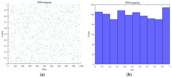
Figure 1.
(a) Frequency value. (b) Frequency mapping.
In Equation (24), there are four scenarios; represents the chaos value of the i iteration; is the modulo operation; if and , the system is in a chaotic state.
(2) Levy Flight
Levy flight is a type of random wandering with a probability distribution of step sizes proposed by the French mathematician Levy, a probability distribution with heavy-tailed properties, where relatively large step sizes occur more frequently than with a normal distribution or other common distributions, which allows for Levy flights to explore more of the space and increase the diversity of the solution space to be explored. Global exploration using the Levy flight strategy allows for dung beetle individuals to be widely distributed in the search space to improve global optimality finding, avoid falling into local optimal solutions, and increase the speed of convergence, as shown in the Levy flight formulation in Equation (25):
In Equation (26), represents a random number that is uniformly distributed within the range of (0,1), represents a random number that is uniformly distributed within the range of (0,2). The formula for is as follows: in Equation (26), :
The position information of the small dung beetle foraging is updated by the Levy flight strategy to achieve a better balance between local search and global exploration. The position update formula is shown in Equation (27):
(3) Adaptive t-distribution variation
In DBO, individuals tend to quickly aggregate to the neighborhood of the current optimal position in the late iteration, and the search ability of the population is substantially weakened, which makes it easy to fall into the optimal solution. In order to solve this kind of problem, adaptive t-distribution variation strategy is introduced, which can dynamically adjust the degree of variation according to the running state of the algorithm and the adaptability of the individuals, which can help the algorithm to jump out of the local optimum and improve the global search ability, and also can focus on strengthening the local search performance.
The final location information of dung beetle individuals is updated by an adaptive t-distribution variation strategy with a t-distribution probability function shown in Equation (28):
where Γ is for the second type of Euler integral, using the number of iterations n for the parameter degrees of freedom, n affects the shape of the curve, Gaussian variation, and Cauchy variation. Cauchy variation can effectively maintain the diversity in the population, which helps the algorithm to jump out of the local optimal solution and explore the wider solution space, while the Gaussian variation has the ability of stronger local development, which ensures that the convergence of the later stages of the evolution of the convergence speed. The position update formula is shown in Equation (29):
In Equation (29), is the final position information of the dung beetle individual in the t iteration; is the random perturbation term; is the parameter degrees of freedom; as T goes to infinity, it is a Gaussian variation; as T goes to 0, it is a Cauchy variation.
By introducing the above improvement ideas into the standard DBO algorithm, the flowchart of the MSDBO optimization algorithm constructed in this paper is obtained as shown in Figure 2.
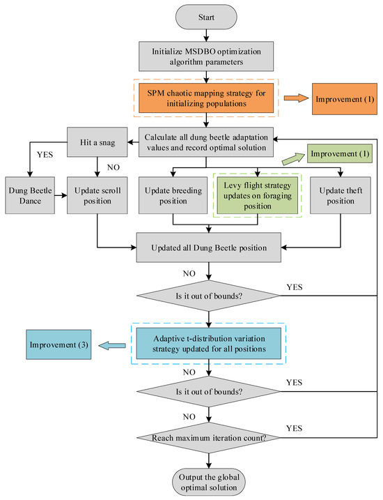
Figure 2.
MSDBO process.
2.4. Prediction Model
2.4.1. Nons-Transformer
The Nons-Transformer [37] model is improved based on the Transformer model. It follows the Transformer model architecture with a standard encoder–decoder structure. The encoder is responsible for encoding the input sequence into contextual representations, while the decoder generates the output sequence from the contextual representations. This structure allows for us to track the flow of information through the model during encoding and decoding to understand how the model transforms inputs into outputs. Compared to Transformer, the Nons-Transformer model, shown in Figure 3, consists of two complementary parts: (1) Sequence stability mechanism to attenuate the instability in the time series. (2) Des attention mechanism, which replaces the self-attention mechanism; compared to the convergence of the self-attention mechanism matrix in the different Transformer sequences after stabilizing the historical wind power, the Des attention mechanism reincorporates the non-stable information into the original sequence, which solves the excessive stable problem after the series is directly stabilized in Transformer.
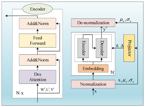
Figure 3.
Nons-Transformer process.
The sequence stability mechanism consists of two corresponding operations. The first one is the normalization module: To attenuate the instability in each input sequence, we normalize the time dimension by means of a sliding window. For each input sequence , it undergoes translation and scaling operations to obtain the output sequence , where S and C denote the length of the sequence and the number of variables, respectively, and the normalization module computation is defined in Equation (30) as follows:
where denotes element-by-element division and denotes element-by-element product. Note that the normalization module reduces the distributional differences between each input time series, making the distribution of model inputs more stable.
Next is the inverse normalization module: As shown in Figure 3, after the basic model predicting the future value of length O, the inverse normalization transformation model is used to output with and , finally obtaining as the final prediction. The inverse normalization module computation is defined in Equation (31):
The implementation of a two-stage transformation allows for the base model to process stable inputs that adhere to a stable distribution, thereby enhancing its generalization capabilities. Furthermore, this design ensures that the model exhibits isovariance with respect to translational and scaling perturbations within the time series, thereby improving its predictive accuracy for the actual series.
To reinstate the initial focus on the non-stable series, we endeavor to reintegrate the diminishing non-stable information into its computational framework. Referring to Equation (32), the primary objective is to approximate the positive scale factor of and the shift vector of , which are designated as Des factors. Given the challenges associated with the rigid linear framework in the context of depth models, and in light of the significant effort required to accurately estimate and leverage the underlying real factors, we propose an alternative approach. Specifically, we aim to directly learn the Des factors from the statistical data of the unsteady states x, Q, and K by employing a straightforward yet effective multilayer perceptron architecture. Given that the available non-stable information is constrained by the current Q′ and K′, the most viable source to address this instability is the un-normalized original dataset x. Consequently, as a direct application of deep learning in accordance with Equation (33), we utilize a multilayer perceptron as a projection mechanism to derive the Des factor from the respective non-stable statistics x and . The formulation of the Des attention mechanism is articulated in Equation (34):
where is the activation function operator, is the attention mechanism operator, and is the multilayer perceptron operator. Equation (31) deduces that except for the current Q′, K′ from stationarized series , this expression also requires the non-stable information that are eliminated by sequence stability mechanism. The Des attention mechanism of all layers share Des factors and . The Des attention mechanism learns the time dependence from both the stable sequence and the non-stable sequence Q′, K′ and multiplies it by the stable value . Thus, it can benefit from the predictability of the stable sequence while maintaining the inherent time dependence of the original sequence.
2.4.2. Nons-DCTransformer
Since the dot product algorithm in the Nons-Transformer model calculates the attention scores between each pair of elements in the sequence in the prediction task, this approach tends to capture global dependencies and is not sensitive enough to the ability to perceive the local environmental features of the sequence, thus limiting the improvement in prediction accuracy. To further reduce the wind power prediction error, convolutional neural networks are introduced to extract features of the local environment. However, the traditional causal convolutional network is a unidirectional structure in which the value before the moment t of the previous layer determines the value of the moment t of the next layer and can map any sequence to an output sequence of the same length. However, the size of the convolutional kernel limits the extraction of features by causal convolution, and longer sense fields or deep network structure stacks are usually required to capture longer correlations, which can lead to the risk of too many parameters, huge computations, and poor fitting. To address these challenges in the prediction task, the encoder part is primarily focused because it is able to convert the input sequence into high-dimensional representations that can then be used for prediction. Therefore, we propose the integration of dilation causal convolution within the Nons-Transformer encoder layer, as illustrated in Figure 4. This approach not only facilitates the capture of local dependencies among wind power sequences across various temporal scales, thereby enhancing model performance, but also mitigates the potential for excessive parameterization and computational demands. The formula for dilation causal convolution is presented in Equation (35):
where * represents the convolution operator, k represents the filter size, and d represents the dilation factor. Distinct from traditional convolution, dilated convolution samples the input at consistent intervals throughout the convolution process, with a dilation factor of d governing the sampling rate.
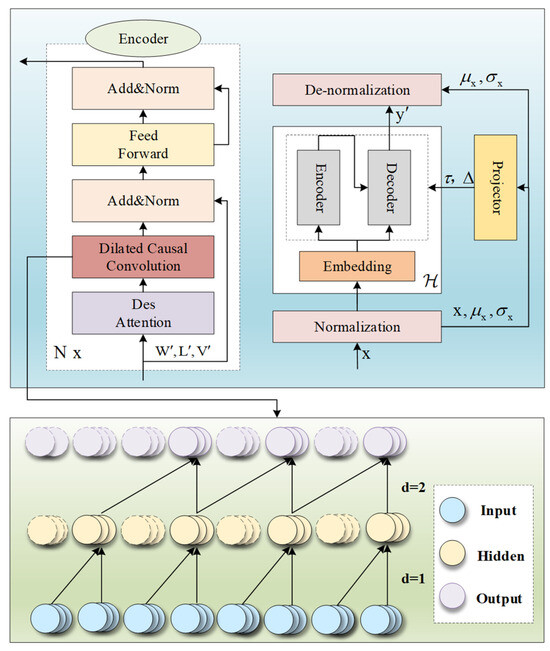
Figure 4.
Nons-DCTransformer process.
3. Establishment of the Proposed Combination Model
The modeling process of the ultra-short-term wind power prediction method with MIVNDN designed in this paper is shown in Figure 5. The main steps are as follows:
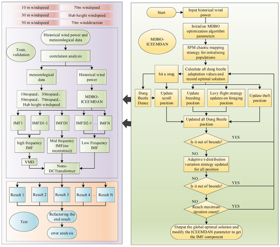
Figure 5.
MSDBO-ICEEMDAN-VMD-Nons-DCTransformer process.
(1) Perform correlation analysis using Spearman’s and Kendall’s correlation coefficients and select a few of the largest correlations between meteorological data and historical wind power as input features. The dataset was divided.
(2) Decompose the historical wind power once by using MSDBO-optimized ICEEMDAN, divide the IMF components of different frequency bands by using sample entropy and t-mean test, reconstruct the high-frequency band and low-frequency band IMF components, leave the middle-frequency band IMF components untouched, and ultimately obtain a high-frequency IMF component, a series of middle-frequency band IMF components, and a low-frequency IMF component.
(3) The high-frequency IMF component is decomposed twice to obtain a series of IMF components.
(4) Utilize a high-frequency IMF component after secondary decomposition, a series of medium-frequency IMF components, and a low-frequency IMF component in the training set, respectively, to establish Nons-DCTransformer prediction models. The early stop mechanism is adopted for the validation set to prevent the problem of poor generalization and overfitting caused by over-training of the training set and saves computing resources and time.
(5) The IMF components corresponding to the test set are fed into the trained prediction model of each component to obtain the predicted values of each component under the test set.
(6) The predicted values corresponding to each IMF component is summed up to obtain the prediction result of the whole historical wind power series and analyze the prediction error by the prediction error evaluation metrics.
4. Case Study
4.1. Data Description and Preprocessing
To validate the effectiveness of the proposed method, a dataset collected from a 96 WM wind farm in Inner Mongolia, China, which covers historical wind power data and meteorological data from 1 January 2019 to 31 December 2019, is used. The dataset consists of 35,037 data points with a sampling interval of 15 min. In addition, preprocessing operations were performed on the collected dataset, including dataset partitioning, data normalization, and prediction data back-normalization.
Firstly, strict division of the dataset can be used both for model evaluation and to avoid future information leakage problems caused by data decomposition. The dataset was divided into training set, testing set, and validation set according to the ratio of 8:1:1. Of the total 80% of the data were used for training, 10% for validation, and 10% for testing, i.e., the first 28,030 sampling points were the training samples, the middle 3504 samples were the validation samples, and the last 3503 samples were the testing samples, which are shown in Figure 6.
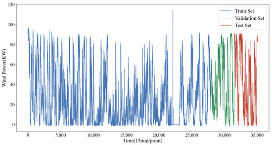
Figure 6.
Historical wind power data.
Secondly, the inputs and outputs of the model are scaled by normalization to obtain the true wind power prediction sequence, which is defined in Equation (36). Finally, the wind power prediction sequence is normalized and after prediction the inverse normalization is carried out to obtain the final wind power prediction sequence, which is defined in Equation (37):
In the above equation, i is the count of sample, is the mean of sample, and is the standard deviation of sample.
4.2. Feature Selection
The dataset contains seven types of data: wind speed at 10 m height, wind speed at 30 m height, wind speed at 50 m height, wind direction at 70 m height, wind speed at 70 m height, wind speed at hub height, and wind power. Not all the above data will necessarily have a significant effect on the wind power prediction, and they will be redundant due to the input features. The redundant features will cause adverse effects such as increase in the model training run time and decrease in the prediction accuracy. Therefore, this paper analyzes the correlation of all kinds of data in the dataset and selects the key input features by correlation coefficients. Since the wind power data have a nonlinear relationship, discontinuity, and do not obey normal distribution, the Spearman’s and Kendall’s correlation coefficient in the correlation evaluation metrics were selected to be analyzed together, and the results are shown in the heat map in Figure 7a,b and Table 1. The judgment criteria of the correlation coefficient are usually 0.8~1.0, indicating strong correlation; 0.6~0.8 indicating strong correlation; 0.4~0.6, indicating moderate correlation; 0.2~0.4, indicating weak correlation; and 0.0~0.2, indicating weak or no correlation. Considering the calculation speed and accuracy, data with a correlation coefficient of 0.6 or more with historical wind power—i.e., wind speed at the height of 10 m, wind speed at the height of 30 m, wind speed at the height of 50 m, wind speed at the height of 70 m, and wind speed at the height of the turbine hub—are selected as input features in this paper, along with historical wind power.
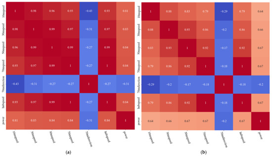
Figure 7.
(a) Spearman’s correlation coefficient; (b) Kendall’s correlation coefficient.

Table 1.
Results of different correlation coefficients.
4.3. Evaluation Indicator
In this research, the evaluation of model performance was conducted using several metrics, including mean absolute error (MAE), mean square error (MSE), root mean square error (RMSE), mean absolute percentage error (MAPE), and the coefficient of determination (R2). MAE quantifies the average of the absolute errors between the predicted and actual values, while MSE calculates the mean of the squared errors, thereby providing insights into both the average and absolute discrepancies between the model’s predictions and the true values; lower values for both metrics indicate superior model performance. RMSE, on the other hand, is the square root of the mean of the squared differences between predicted and actual values, and it is particularly sensitive to larger discrepancies. The coefficient of determination, R2, ranges from 0 to 1 and assesses the model’s fit to the target variable, with values closer to 1 indicating a better fit. The definitions of these five evaluation metrics are provided in Equations (38)–(42):
In the above equation, n is the number of samples, is the predicted value of the model, y is the true value, and is the mean value.
4.4. Experimentation and Analysis
All experiments were realized based on the programming language Python 3.8, MATLAB 2018a, and the deep learning framework Pytorch torch 1.8 on a configuration of an AMD Ryzen 7 7735H 3.20 GHz CPU and NVIDIA 4060 8G GPU.
4.4.1. Comparative Experimental Analysis of Optimization Algorithms
To evaluate the effectiveness of the proposed enhancement to the algorithm, the northern goshawk optimization algorithm (NGO), gray wolf optimization algorithm (GWO), whale optimization algorithm (WOA), DBO, and MSDBO algorithms were used to optimize the fitness curves, including optimal values, means, and standard deviations of the ICEEMDAN, as detailed in Table 2. For a fair and efficient comparison, each algorithm was set up with 8 individuals, a maximum of 10 iterations, an upper bound of [0.1,30], a lower bound of [0.3,60], and a dimension of 2. The sample entropy of the final IMFN component, derived from the wind power decomposition via ICEEMDAN, served as the fitness function (with the residual term defined as the IMFN component). The maximum number of iterations for ICEEMDAN was set at 500, and the NSTD and NE parameter combinations were explored. Figure 8 illustrates the optimization iteration process for the five algorithms.
Table 2.
Results of optimization search with different optimization algorithms.
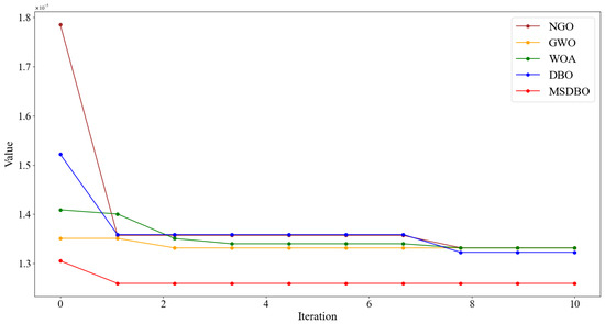
Figure 8.
Comparison of optimization algorithms.
The comparative analysis presented in Figure 8 indicates that NGO initially achieves the highest fitness value, suggesting its global search capability is limited and prone to local optima. Conversely, GWO starts with a lower fitness value but shows less convergence performance compared to WOA and DBO as iterations continue. Among the various convergence curves, MSDBO stands out with the fastest convergence rate and the highest optimization accuracy. Additionally, a closer look at the data in Table 2 reveals that MSDBO significantly outperforms WOA and DBO in terms of optimum, mean, and standard deviation, attributed to the SPM chaotic mapping’s ability to quickly identify the global optimal solution. Through its iterations, MSDBO efficiently locates the lowest fitness value, thanks to the incorporation of the Levy flight strategy and adaptive t-distribution variation, which enhance its global search and convergence capabilities. In summary, with its unique design and innovative algorithm strategy, MSDBO achieves high convergence accuracy while maintaining convergence speed, and sufficiently balances global and local search capabilities. In addition, the fitness function of various optimization algorithms chooses the sample entropy of ICEEMDAN decomposition to the final IMF component, which is the optimization of parameter combination in noisy data or uncertain environment. Combined with the above results, it proves that MSDBO algorithm also shows strong anti-noise ability and adaptability.
4.4.2. Experimental Analysis of Quadratic Decomposition Reconstruction Strategy
The parameters of the ICEEMDAN method are all set artificially, and blindly setting the parameters cannot bring out the best performance of the algorithm [38]. Since the decomposition effect of the ICEEMDAN method depends on the parameters NSTD and NE, MSDBO is introduced to optimize the search of the parameter combinations of ICEEMDAN to achieve the purpose of adaptive optimal setting of the parameters and to improve the ability of extracting the features by using MSDBO-ICEEMDAN to reject the noise in the wind power. Initialize the MSDBO optimization algorithm parameters, configured with eight individuals. The maximum number of iterations is 10, and the sample entropy of the last IMFN component after ICEEMDAN decomposition of wind power is taken as the fitness function. When the fitness value is smaller, it represents the smaller complexity of decomposition to the last IMFN component, which can better prevent the difficulty of modeling caused by the stacking of the IMF components being too large. Given that the ICEEMDAN parameter combination of NSTD and NE has an upper bound of [0.1, 30] and a lower bound of [0.3, 60], the maximum number of iterations is 500. The final optimal parameter combinations of NSTD and NE are determined through optimization and updating, and the ICEEMDAN parameters are reconfigured to set the NSTD to 0.23 and the NE to 60. This is followed by using ICEEMDAN with the determined optimal parameter combination to model the historical wind power and generate 14 IMF components. The spectrum is shown in Figure 9, with the first row representing the historical wind power.
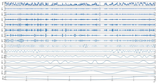
Figure 9.
MSDBO-ICEEMDAN primary decomposition spectrum results.
Since the components generated by ICEEMDAN have the property that the mean value is approximately 0, the frequency of each component decreases sequentially, and the components are independent of each other, this paper utilizes the t-test to test the 0-mean hypothesis for each IMF component by setting up a two-sided hypothesis: The original hypothesis H0: the mean value of the IMF components = 0. The alternative hypothesis H1: the mean value of the IMF components ≠ 0. Taking the significance level of 0.05, i.e., when the p-value is greater than the selected level of significance, the original hypothesis H0 is accepted; otherwise, the alternative hypothesis H1 is accepted.
In general, when calculating sample entropy, m takes 1 or 2, and it is more common for m to be set to 2. Because this can better capture the dynamic properties in the time series, we set m to 2 here. Common values for r range from 0.1 to 0.25 times the standard deviation of the time series. When the value of r is large, more information is lost because more pairs of vectors are considered similar. However, when the value of r is small, it is not ideal to estimate the statistical properties of the system, because many actually similar vector pairs may be excluded due to small differences, so we set r to 0.2 times the time series standard deviation here.
At the significance level of 0.05, the t-test is conducted for the difference in means of each IMF component and the respective sample entropy is calculated, as shown in Table 3 and Table 4, where it can be seen that at IMF6, the p-value is less than 0.05 for the first time, which is significant, and at IMF11, the p-value is less than 0.05 for the second time, which is significant. In the meantime, by the monotonically decreasing result of sample entropy, as shown in Figure 10, the complexity of the IMF components is monotonically reduced, so the frequency is monotonically reduced. Therefore, these two places are taken as the demarcation points of different frequency band IMF components: IMF1-IMF5 are the high-frequency band IMF components, IMF6-IMF10 are the middle-frequency band components, and IMF11-IMF14 are the low-frequency band components.
Table 3.
Sample entropy and p-value results 1–7.
Table 4.
Sample entropy and p-value results 8–14.
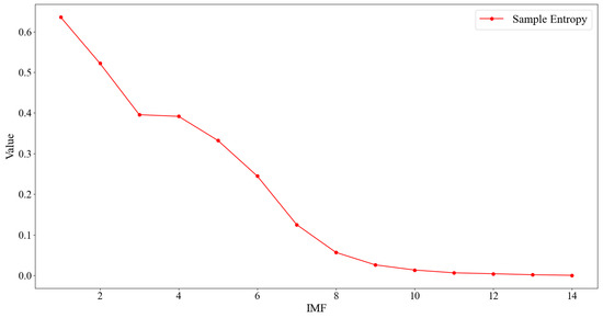
Figure 10.
Sample entropy results.
The IMF components of the high-frequency band, middle-frequency band, and low-frequency band are obtained from the sample entropy and t-mean test. Given that the middle-frequency band IMF component after one decomposition has moderate complexity and less noise, in order to retain the important feature information of the original signal in the band, it is not subjected to any additional reconstruction or processing but is directly inputted into the model as a feature, which ensures that the model can adequately learn the key information of the frequency band. The considered high-frequency band IMF components still contain high complexity and residual noise components, which are reconstructed by summing to obtain a single high-frequency IMF component, and then the reconstructed high-frequency IMF components are decomposed twice.
The value of K in VMD influences the effectiveness of the decomposition, and it is typically determined based on expert judgment, usually ranging from 5 to 9. In this case, we assess the value of K by calculating the central frequency of the IMF components. The optimal K value is achieved when eventually the central frequency of the IMF component tends to stabilize. As shown in Table 5, when K is set to 8 and 9, the last IMF component’s central frequency is closest to that of the preceding IMF component, indicating stability. Therefore, we choose K to be 8 to generate a new set of IMF components, and the obtained IMF spectrum is shown in Figure 11, with the first row as the historical wind power, which aims to further refine the structure of the IMF components, so that the high-frequency features and noise components can be separated on a smaller scale, reducing the interference of noise on the model performance, lowering the modeling difficulty, and improving the accuracy of the prediction. For the IMF components in the lower frequency bands, they are summed and reconstructed to simplify the modelling process and reduce the amount of computation, since their influence on the prediction results is minimal.
Table 5.
The center frequency of different mode number.
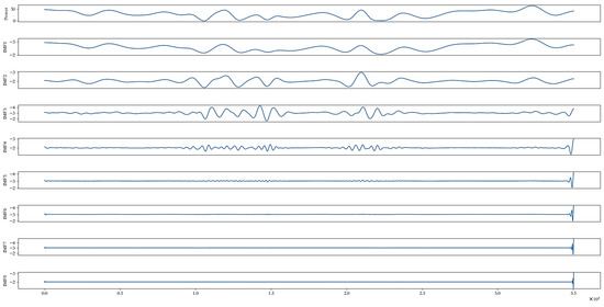
Figure 11.
VMD quadratic decomposition spectrum.
To verify the effectiveness of the quadratic decomposition reconstruction strategy, we designed a series of models with different quadratic decomposition reconstruction strategies to compare with ours(our model), and analyzed the five error metrics of MAE, MSE, RMSE, MAPE, and R2. The statistical results of the error metrics evaluations are shown in Table 6: model A (without secondary decomposition reconstruction, directly using Nons-DCTransformer to predict different frequency band IMF components after primary decomposition above), model B (without secondary decomposition, both high-frequency band IMF components and low-frequency band IMF components are reconstructed, and the middle-frequency band IMF is not reconstructed; then, Nons-DCTransformer is utilized to predict the above components), model C (the high-frequency band IMF components are reconstructed, middle-frequency band IMF components are not reconstructed, and the low-frequency band IMF is reconstructed; the low-frequency band IMF is reconstructed after primary decomposition), and model D (the high-frequency band and low-frequency band components are both reconstructed and then decomposed twice, the mid-frequency band IMF component is not reconstructed, and the above components are predicted using Nons-DCTransformer).
Table 6.
Evaluation metrics for different secondary decomposition reconstruction strategies.
To compare the prediction efficacy of different models more intuitively and efficiently, we chose radargrams for in-depth analysis. From Figure 12, we can see that different decomposition and reconstruction methods have a great impact on the prediction performance, and reconstructing the high-frequency band IMF components or the secondary decomposition of the reconstructed high-frequency IMF components can effectively improve the prediction accuracy. In combination with the evaluation metrics, ours reduces the MAE, MSE, RMSE, and MAPE relative to model A by 31.81%, 56.34%, 56.34%, 33.86%, and 27.63%, respectively, while the R2 improves by 0.92%. The MAE, MSE, RMSE, and MAPE relative to model B decrease by 41.24%, 68.27%, 43.71%, and 32.67%, while the R2 improves by 1.64%. The low-frequency band IMF component reconstruction or the secondary decomposition of the reconstructed components has a negligible effect on the model performance, and the performance of model B and model C in the metrics of MAE, MSE, RMSE, MAPE, and R2 is almost comparable with a negligible difference. Meanwhile, ours also presents extremely close results in these metrics compared to model D. However, ours still dominates and leads in these similar metrics. In summary, to improve the model performance and to reduce the experimental procedure, we selected the secondary decomposition of the reconstructed high-frequency IMF components and the reconstruction of the low-frequency band IMF components as our final modeling strategy.
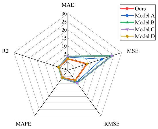
Figure 12.
Radar chart of evaluation indicators reconstructed by secondary decomposition.
4.4.3. Experimental Analysis of Ablation
In this paper, ablation experiments were designed to evaluate the performance gains included in the testing of each module in ours, comparing this model with model 1 (Transformer), model 2 (Nons-Transformer), model 3 (Nons-DCTransformer), model 4 (ICEEMDAN- Nons- DCTransformer), and model 5 (MSDBO-ICEEMDAN-Nons-DCTransformer); we also compared the models constructed with different input features, and the results of the evaluation metrics are shown in Table 7 and Figure 13a,b.
Table 7.
Ablation experiments evaluation indicators metrics.
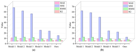
Figure 13.
(a) Single-model evaluation metrics; (b) combined model evaluation metrics.
Table 7 clearly shows that the benchmark model 1 has the highest MAE. In contrast, our model demonstrates reductions in MAE, MSE, and RMSE by 66.43%, 88.09%, and 65.49%, respectively, while R2 increases by 5.87%. Additionally, when observing the fitting figure of the prediction curve alongside the actual curve in Figure 14, it is evident that our model is more adept at capturing the intricate relationships within the data, leading to enhanced overall prediction performance compared to the benchmark model.
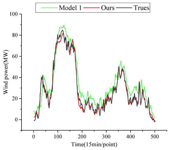
Figure 14.
Benchmark model comparison.
In the ablation experiments, we set the learning rate of the ablation experimental model to 0.0001, the batch size to 32, the hidden layer size to 512, the dropout to 0.1, the output size to 8, the model dimensionality to 512, the encoder layer to 2, the decoder layer to 1, the number of training rounds to 10, and the mapping layer dimensions unique to the Nons-Transformer architecture to 256, 256; the number of layers is 2.
A comparison between model 1 and model 2 reveals that the decomposition of MAE, MSE, and RMSE is reduced by 17.27%, 9.88%, and 5.11%, respectively, while R2 is improved by 0.75%. The substitution of the attentional mechanism in the Transformer with the Des attentional mechanism effectively alleviates the excessive stable problem caused by Transformer and its variants on the direct stability of historical wind power data, thereby improving the prediction performance.
When comparing model 2 and model 3, the incorporation of dilation causal convolution within the encoder not only prevents information leakage but also introduces a dilation factor that enhances the model’s sensitivity to local features across varying time scales, resulting in improved accuracy. This is evidenced by reductions in MAE, MSE, and RMSE by 10.26%, 9.54%, and 4.88%, respectively, alongside a 0.53% increase in R2.
The comparison between model 3 and model 4 demonstrates that the inclusion of ICEEMDAN in the predictive model significantly decreases prediction errors, with reductions of 26.38%, 60.00%, and 36.60% for MAE, MSE, and RMSE, respectively, and an improvement in R2 by 3.16%. This enhancement is attributed to ICEEMDAN’s capability to decompose historical wind data into IMF components across various frequency ranges, thereby enabling the predictive model to predict wind power at multiple frequency scales, which ultimately increases accuracy and reduces error.
Comparison between model 4 and model 5 shows that the MSDBO optimized ICEEMDAN has some performance improvement compared to the direct decomposition of historical wind power prediction without optimization, with the MAE, MSE, and RMSE reduced by 6.78%, 8.16%, and 4.16%, respectively, and the R2 improved by 0.21%. This shows that the choice of NSTD and NE combinations in ICEEMDAN has some effectiveness and emphasizes the importance of ICEEMDAN parameter optimization.
By comparing model 5 with ours, the reconstructed low-frequency band IMF component reduces the experimental process, and the secondary decomposition of the reconstructed high-frequency IMF component using VMD further removes the noise and reduces the modeling difficulty, which in turn reduces the prediction errors such as by MAE, MSE, and RMSE by 23.46%, 43.99%, and 25.18%, respectively, and R2 improved by 0.82%, which effectively improves the model performance.
By comparing ours constructed based on inputs of seven features versus six features, we find that input features with low correlation lead to model redundancy; selecting key input features using Spearman and Kendall correlation coefficients reduces the prediction error; the MAE, MSE, and RMSE are reduced by 13.92%, 13.92%, and 16.00%, respectively; and the R2 improves by 0.30%.
In summary, Nons-Transformer effectively solves the excessive stable problem affecting model performance due to the “direct stability” design of the Transformer and its variants; the inclusion of dilated causal convolution in the Nons-Transformer encoder improves the perception of local features; ICEEMDAN reduces the noise, effectively reduces the complexity of the WT historical data, and enhances the readability of the data; the proposed MSDBO method not only makes full use of the theoretical basis of the ICEEMDAN process, but also significantly improves the decomposition effect. The Spearman and Surel correlation coefficients screen out the most critical input features, thus reducing redundancy and improving prediction accuracy. In addition, considering that the IMF high-frequency band component still retains participation noise with high complexity and modelling difficulty, and that the low-frequency band component does not affect the prediction effect, the high-frequency and low-frequency bands are reconstructed by the sample entropy and t-mean test and the high-frequency component is decomposed secondarily, which effectively improves the prediction accuracy and reduces the experimental process. The analysis of the ablation experiments shows that ours has performance gains in each module, and these modules work together for the ultra-short-term wind power prediction task to significantly improve the prediction accuracy and robustness.
4.4.4. Comparative Experimental Analysis
To assess the validity and stability of ours, we designed twelve comparative experiments and the fitting diagrams are shown in Figure 15a,b including single model a (BP), model b (CNN), model c (LSTM), model d (GRU), model e (BiLSTM), and model f (TCN), and combined model g (CNN-LSTM), model h (EMD-Nons-DCTransformer), model i (VMD-Nons-DCTransformer), model j (WOA-ICEEMDAN-VMD-Nons-DCTransformer), model k (DBO-ICEEMDAN-VMD-Nons-DCTransformer), and model l (MSDBO-ICEEMDAN-EMD-Nons-DCTransformer). Table 8 details the results of each evaluation metric, and Figure 16 demonstrates the MAE metrics of different models, providing us with a rich basis for comparative analysis.

Figure 15.
(a) Single-model comparison; (b) combined model comparison.
Table 8.
Overall comparison experiment evaluation metrics.
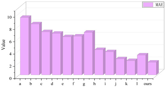
Figure 16.
Comparative test MAE.
During the comparison, it was observed that model a exhibited relatively weak predictive capabilities, which can be attributed to its limitations in feature extraction inherent to deep neural network architectures, thereby restricting its applicability in wind power prediction. Although CNNs demonstrate strong performance in image processing, their effectiveness in time-series prediction is not as pronounced. Commonly utilized models in the time-series prediction domain, such as LSTM, BiLSTM, GRU, and TCN, may also fall short of anticipated predictive outcomes due to insufficient sensitivity to local features. Furthermore, model d outperformed model h and i in terms of decomposition methodology, with reductions in MAE, MSE, and RMSE of 21.97%, 47.92%, and 27.86% when compared to model h, and 18.38%, 25.75%, and 13.84% when compared to model i, respectively. Additionally, the R2 values for model d improved by 1.77% and 0.62%, respectively. Ours also demonstrated a significant advantage over the EMD quadratic decomposition algorithm utilized in model l, as evidenced by substantial reductions in MAE, MSE, and RMSE, alongside notable improvements in R2.
Specifically, ours achieved reductions in the evaluation metrics MAE, MSE, and RMSE of 20.82%, 33.89%, and 18.69% compared to model j, and 10.88%, 18.80%, and 9.90% compared to model k, while enhancing the R2 metrics by 0.40% and 0.20%, respectively. This marked advantage is primarily due to the MSDBO-ICEEMDAN decomposition algorithm’s exceptional capability for pattern separation, which is facilitated by the precise optimization of NSTD and NE parameter combinations, effectively mitigating noise and enhancing the quality of the decomposition results. Moreover, the incorporation of dilated causal convolution and a Des attention mechanism further augments the model’s proficiency in local feature extraction and addresses the problem where the sequence is excessively stable, which affects model performance. In summary, our proposed Nons-DCTransformer ultrashort-term wind power prediction model based on the secondary decomposition reconstruction strategy successfully integrates the advantages of MSDBO-ICEEMDAN primary decomposition, secondary decomposition reconstruction strategy, and a Nons-DCTransformer model. This integration strategy enables the model to more accurately capture the short-term and long-term dependencies of wind power sequence, which significantly improves the prediction accuracy. This result not only verifies the validity and stability of the model, but also provides new research ideas and methods in the field of wind power prediction.
4.4.5. Experimental Analysis of Wind Power for Some of More Stable and Sharply Fluctuating Wind Power
In wind farms, due to meteorological instability and other factors, there are dramatic changes in wind power, leading to sharp rises and falls. At this time, accurately predicting wind power is one of the problems that need to be solved. The selection of the historical wind power data of sharp rise and fall in wind farm to reflect the proposed combination model for generalization to different wind power situations, which includes a total of 200 test data points outside the training set, as shown in Figure 17, with a time interval of 15 min. Additionally, part of the more stable historical wind power data in wind farm is selected, which also includes a total of 200 test data points outside the training set, as shown in Figure 18, with a time interval of 15 min. The models are compared through experimental analysis of the two different historical power data and the same moment of the meteorological data prediction to verify the robustness of a variety of models. The power prediction fitting diagrams of the two stages are shown in Figure 19a,b and Figure 20a,b, respectively, and the evaluation metrics are shown in Table 9 and Table 10.
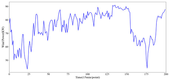
Figure 17.
Dramatic fluctuations in historical wind power sequence.
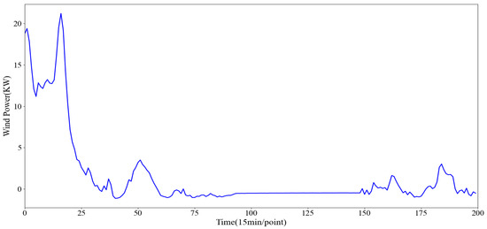
Figure 18.
More stable historical wind power sequence.
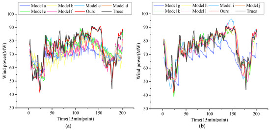
Figure 19.
(a) Single model; (b) combined model.
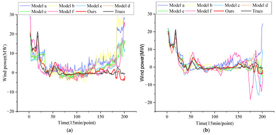
Figure 20.
(a) Single model; (b) combined model.
Table 9.
Comparison experiment evaluation metrics.
Table 10.
Comparison experiment evaluation indicators.
(1) Dramatically fluctuating wind power sequence
By observing Figure 19a,b, it can be clearly seen that under the scenario of wind power experiencing drastic and sharp rise and fall, for example, when the time series data are located in the interval from 0 to 150, ours demonstrates a very high degree of fit, and its prediction curves almost overlap with the historical wind power curves, which closely fits the actual trend of change.
Further, when the historical wind power is in the critical phase of sharp rise and fall, especially in the range of time series data from 150 to 200, ours still maintains the excellent performance. Compared to other comparative models, it not only captures the sharp changes in wind power more accurately, but also demonstrates significant advantages in prediction accuracy and stability.
To summarize, ours shows remarkable predictive ability and robustness in dealing with the challenges of complex and variable wind power with sharp rise and fall, which provides a strong support for the accurate prediction of wind power.
(2) Relatively stable wind power sequence
An examination of Figure 20a,b reveals that, in scenarios characterized by relatively stable wind power, ours exhibits exceptional accuracy, with its prediction curves closely aligning with the actual wind power output curves, thereby indicating a high degree of fit.
In this specific dataset for prediction, ours outperforms other comparative models in terms of wind power prediction capabilities. It not only significantly surpasses them in prediction accuracy but also demonstrates a consistent level of stability and reliability throughout the prediction process, thereby ensuring precise wind power predictions.
In conclusion, ours also shows commendable performance in scenarios involving more stable wind power. Its accurate predictive capabilities and high stability offer substantial support for the reliable operation and effective management of the wind power sector.
5. Conclusions
In this paper, an ultra-short-term wind power prediction method with MIVNDN is proposed. Our proposed combined model includes the following: (1) the MSDBO-ICEEMDAN algorithm aims to analytically decompose the historical wind power series into a set of IMF components with different frequency ranges; (2) the high-frequency band and low-frequency band IMF components are reconstructed through sample entropy and t-mean test, and the reconstructed high-frequency IMF components are subjected to quadratic decomposition in order to further refine their characteristics; (3) we combine the quadratic decomposed IMF component, the unreconstructed mid-frequency band component, and the reconstructed low-frequency IMF component as inputs, and use the Nons-DCTransformer model to make ultra-short-term wind power prediction, i.e., wind power prediction in the next 2 h; (4) by comparing the prediction with different single and combined models on the real data collected from a 96 WM wind farm in Inner Mongolia, ours is able to predict the wind power in the next 2 h, which is the same as that in the next 2 h. Ours reduces 77.63%, 75.03%, 70.48%, 69.09%, 66.61%, and 66.85% compared to the single model a, b, c, d, e, and f, respectively, and the combined model g, h, i, j, k, and l reduces 69.83%, 50.15%, 47.85%, 20.82%, 10.89%, and 35.92%, respectively. To sum up, wind power is non-stable and uncertain, which poses a challenge to the stable operation of the power system. By integrating improved optimization algorithms, data processing methods, decomposition and reconstruction strategy, and improved prediction model, our model aims to provide a more accurate and robust ultra-short-term wind power prediction method, reducing wind power prediction errors, and improving the scheduling flexibility and reliability of power grids, which has important research value and practical application prospects. The important conclusions of this work are as follows:
(1) The optimal parameter combination of NSTD and NR for ICEEMDAN decomposition of wind power sequence can be searched faster by MSDBO, which improves the denoising ability and decomposition effect of ICEEMDAN, also shows strong anti-noise ability and adaptability.
(2) The secondary decomposition and reconstruction strategy effectively reduces the interference of the noise on the performance of the model, reduces the difficulty of modeling, and simplifies the experimental process, and significantly improves the accuracy of prediction.
(3) The Des attention mechanism together with the sequence stability mechanism solves the excessive stable problem of the Transformer model by directly stabilizing the data and introduces the dilated causal convolution to extract the features of the local environment, which improves the prediction accuracy.
(4) Ours has a variety of feature extraction capabilities, can capture the short-term changes in the wind power series, and performs equally well in dealing with the complexity and variability of wind power, sharp rise and fall, and stable wind power scenarios, and has a better prediction accuracy and stability compared with other models. This demonstrates that the model has strong generalization capabilities and applicability, suggesting its potential value in other forecasting fields.
However, our combined model also has some limitations. The manual trial-and-error method to select the hyperparameters of the model is inefficient and may find feasible but non-optimal solutions, which may hinder the realization of more accurate predictions. In addition, we did not consider the applicability of the model in different seasons and regions during the experiment. In the future, we will continue to study the general applicability of the wind power prediction model and ensure the efficiency of the prediction while keeping the prediction accuracy.
Author Contributions
Conceptualization, L.G. and X.R.; Methodology, Q.Z.; Writing—original draft Q.Z.; Writing—review and editing, Q.Z. and L.G.; Validation, F.Z.; Formal analysis, L.Q.; Visualization, Y.W. All authors have read and agreed to the published version of the manuscript.
Funding
This work was supported by The National Natural Science Foundation of China (62161041), Inner Mongolia Natural Science Foundation (2022SHZR0375), and Inner Mongolia Autonomous Region Science and Technology plan project (2021GG0046).
Data Availability Statement
Data are available on request to the authors.
Conflicts of Interest
The authors declare no conflict of interest.
References
- Jin, M. Research on Wind Power Prediction Based on Improved VMD and Deep Learning; Xi’an University of Technology: Xi’an, China, 2023. [Google Scholar]
- Sun, X.; Liu, H. Multivariate short-term wind speed prediction based on PSO-VMD-SE-ICEEMDAN two-stage decomposition and Att-S2S. J. Energy 2024, 305, 132228. [Google Scholar] [CrossRef]
- Zhou, W. Research on Wind Power Prediction Method Based on BiGRU-Att-1dCNN Model; Shenyang Institute of Technology: Shenyang, China, 2023. [Google Scholar] [CrossRef]
- Yang, T.; Yang, Z.; Li, F.; Wang, H. A short-term wind power forecasting method based on multivariate signal decomposition and variable selection. J. Appl. Energy 2024, 360, 122759. [Google Scholar] [CrossRef]
- Deng, Y. Research and Application of Wind Power Prediction Based on Deep Learning; Guangzhou University: Guangzhou, China, 2024. [Google Scholar] [CrossRef]
- Zang, Y.; Nong, G.; Zhang, Z.; Lin, L. Ultra-short term wind power prediction based on improved spatial density clustering. J. Jilin Inst. Chem. Technol. 2023, 40, 32–37. [Google Scholar] [CrossRef]
- Chenjia, H.; Yan, Z.; He, J.; Mingkun, J.; Fucai, Y.; Qian, L. Prediction of ultra-short-term wind power based on CEEMDAN-LSTM-TCN. J. Energy Rep. 2022, 8, 483–492. [Google Scholar] [CrossRef]
- Zhao, Y. Research on Ultra-Short Term Wind Power Prediction Based on Attention Mechanism; Taiyuan University of Technology: Taiyuan, China, 2023. [Google Scholar] [CrossRef]
- Li, S. Research on Ultra-Short Term Wind Power Probability Prediction Considering the Correlation of Meteorological Factors; Shenyang University of Technology: Shenyang, China, 2022. [Google Scholar]
- Chuang, W.Z.; Cai, N.J. Wind power output prediction: A comparative study of extreme learning machine. J. Front. Energy Res. 2023, 11, 1267275. [Google Scholar] [CrossRef]
- Shi, J.; Liu, Y.; Yang, Y.; Han, S.; Wang, P. The research and application of wavelet-support vector machine on short-term wind power prediction. In Proceedings of the 2010 8th World Congress on Intelligent Control and Automation, Jinan, China, 7–9 July 2010; pp. 4927–4931. [Google Scholar] [CrossRef]
- Ling, X.; Jianing, L.; Xin, Y.; Aijun, H.; Hao, S. Ultra-short term wind power prediction applying a novel model named SATCN-LSTM. J. Energy Convers. Manag. 2022, 252, 115036. [Google Scholar] [CrossRef]
- Zhu, A.; Li, X.; Mo, Z.; Wu, R. Wind power prediction based on a convolutional neural network. In Proceedings of the 2017 International Conference on Circuits, Devices and Systems (ICCDS), Chengdu, China, 5–8 September 2017; pp. 131–135. [Google Scholar] [CrossRef]
- Zhu, Q.; Li, H.; Wang, Z.; Chen, J.; Wang, B. Short-term wind power forecasting based on LSTM. Power Syst. Technol. 2017, 41, 3797–3802. [Google Scholar] [CrossRef]
- Wang, Y.; Zeng, X.; Gao, G. Wind power short-term prediction model based on GRU network. J. Instrum. Technol. 2020, 39, 9–12+39. [Google Scholar] [CrossRef]
- Bai, S.; Kolter, J.Z.; Koltun, V. An empirical evaluation of generic convolutional and recurrent networks for sequence modeling. arXiv 2018, arXiv:1803.01271. [Google Scholar] [CrossRef]
- Siami-Namini, S.; Tavakoli, N.; Namin, A.S. The performance of LSTM and BiLSTM in forecasting time series. In Proceedings of the 2019 IEEE International Conference on Big Data (Big Data), Los Angeles, CA, USA, 9–12 December 2019; pp. 3285–3292. [Google Scholar] [CrossRef]
- Vaswani, A.; Shazeer, N.; Parmar, N.; Uszkoreit, J.; Jones, L.; Gomez, A.N.; Kaiser, L.; Polosukhin, I. Attention is all you need. arXiv 2017, arXiv:1706.03762. [Google Scholar] [CrossRef]
- Wang, L.; He, Y.; Li, L.; Liu, X.; Zhao, Y. A novel approach to ultra-short-term multi-step wind power predictions based on encoder–decoder architecture in natural language processing. J. Clean. Prod. 2022, 354, 131723. [Google Scholar] [CrossRef]
- Keneshloo, Y.; Shi, T.; Ramakrishnan, N.; Reddy, C.K. Deep reinforcement learning for sequence-to-sequence models. IEEE Trans. Neural Netw. Learn. Syst. 2019, 31, 2469–2489. [Google Scholar] [CrossRef] [PubMed]
- Huang, X. Research on Wind Power Prediction Based on Combination Model; Hunan University of Technology: Zhuzhou, China, 2023. [Google Scholar] [CrossRef]
- Chen, X. Ultra Short Term Wind Power Prediction Based on ISA-LSTM; Ningxia University: Yinchuan, China, 2022. [Google Scholar] [CrossRef]
- Ma, Z.; Wu, T.; Guo, S.; Wang, H.; Xu, G.; Aziz, S. An integrated prediction model based on meta ensemble learning for short-term wind speed forecasting. IEEE Access. 2024, 1–11. [Google Scholar] [CrossRef]
- Cheng, Y.; Guang, Y.; Cheng, Y.; Yu, Z.; Xi, M. A multi-factor driven spatiotemporal wind power prediction model based on ensemble deep graph attention reinforcement learning networks. J. Energy 2023, 263, 126034. [Google Scholar] [CrossRef]
- Hu, M.; Zheng, G.; Su, Z.; Kong, L.; Wang, G. Short-term wind power prediction based on improved variational modal decomposition, least absolute shrinkage and selection operator, and BiGRU networks. Energy 2024, 303, 131951. [Google Scholar] [CrossRef]
- Wang, X.; Shen, X.; Ai, X.; Li, S. Short-term wind speed forecasting based on a hybrid model of ICEEMDAN, MFE, LSTM and informer. PLoS ONE 2023, 18, e0289161. [Google Scholar] [CrossRef]
- Yang, Y.; Zhang, Y. Based on the mRMR and VMD-AM-short-term wind power prediction LSTM. J. Control Eng. 2022, 29, 10–17. [Google Scholar] [CrossRef]
- Peng, S.; Zhu, J.; Wu, T.; Yuan, C.; Cang, J.; Zhang, K.; Pecht, M. Prediction of wind and PV power by fusing the multi-stage feature extraction and a PSO-BiLSTM model. Energy 2024, 298, 131345. [Google Scholar] [CrossRef]
- Liu, Y.; Wu, S.; Zhu, Y.; Yang, P.; Sun, T. Ultra-short-term prediction of wind power based on CEEMDAN and DBO-GRNN. J. Electr. Power Constr. 2024, 45, 97–105. [Google Scholar] [CrossRef]
- Liu, J.; Cong, L.; Xia, Y.; Pan, G.; Zhao, H.; Han, Z. Short-term power load forecasting based on the combination model of DBO-VMD and IWOA-BILSTM neural networks. J. Power Syst. Prot. Control 2024, 52, 123–133. [Google Scholar] [CrossRef]
- Colominas, M.A.; Schlotthauer, G.; Torres, M.E. Improved complete ensemble EMD: A suitable tool for biomedical signal processing. J. Biomed. Signal Process. Control 2014, 14, 19–29. [Google Scholar] [CrossRef]
- Dragomiretskiy, K.; Zosso, D. Variational mode decomposition. IEEE Trans. Signal Process. 2013, 62, 531–544. [Google Scholar] [CrossRef]
- Pu, X. Ultra-Short Term Wind Power Prediction Based on Two-Layer Decomposition and LSTM; Kunming University of Science and Technology: Kunming, China, 2021. [Google Scholar] [CrossRef]
- Zhou, X. Research on Ultra-Short Term Wind Power Prediction Method Based on Quadratic Decomposition and Machine Learning; Southwest Jiaotong University: Chengdu, China, 2021. [Google Scholar] [CrossRef]
- Jiankai, X.; Bo, S. Dung beetle optimizer: A new meta-heuristic algorithm for global optimization. J. Supercomput. 2023, 79, 7305–7336. [Google Scholar] [CrossRef]
- Wang, Z.; Wang, S.; Cheng, Y. Fault Feature Extraction of Parallel-Axis Gearbox Based on IDBO-VMD and t-SNE. J. Appl. Sci. 2023, 14, 289. [Google Scholar] [CrossRef]
- Liu, Y.; Wu, H.; Wang, J.; Long, M. Non-stationary transformers: Exploring the stationarity in time series forecasting. Adv. Neural Inf. Process. Syst. 2022, 35, 9881–9893. [Google Scholar] [CrossRef]
- Chen, A.; Wang, H. Fault diagnosis of planetary gearbox based on HBA-ICEEMDAN and HWPE. J. Mechatron. Eng. 2023, 40, 1157–1166. [Google Scholar] [CrossRef]
Disclaimer/Publisher’s Note: The statements, opinions and data contained in all publications are solely those of the individual author(s) and contributor(s) and not of MDPI and/or the editor(s). MDPI and/or the editor(s) disclaim responsibility for any injury to people or property resulting from any ideas, methods, instructions or products referred to in the content. |
© 2024 by the authors. Licensee MDPI, Basel, Switzerland. This article is an open access article distributed under the terms and conditions of the Creative Commons Attribution (CC BY) license (https://creativecommons.org/licenses/by/4.0/).