Applications of Machine Learning in Cancer Imaging: A Review of Diagnostic Methods for Six Major Cancer Types

Abstract

Machine learning (ML) methods have revolutionized cancer analysis by enhancing the accuracy of diagnosis, prognosis, and treatment strategies. This paper presents an extensive study on the applications of machine learning in cancer analysis, with a focus on three primary areas: a comparative analysis of medical imaging techniques (including X-rays, mammography, ultrasound, CT, MRI, and PET), various AI and ML techniques (such as deep learning, transfer learning, and ensemble learning), and the challenges and limitations associated with utilizing ML in cancer analysis. The study highlights the potential of ML to improve early detection and patient outcomes while also addressing the technical and practical challenges that must be overcome for its effective clinical integration. Finally, the paper discusses future directions and opportunities for advancing ML applications in cancer research.

1. Introduction

Globally, cancer continues to be a significant public health challenge, with nearly 20 million new cases and 9.7 million deaths that occurred in 2022 alone [1]. In 2024, the American Cancer Society estimated there would be 2,001,140 new cancer cases and 611,720 cancer-related deaths. The projected 611,720 deaths translate to approximately 1671 fatalities daily, with lung, prostate, and colorectal cancers being the primary causes in men, and lung, breast, and colorectal cancers being the primary causes in women [2]. These data underscore the ongoing challenges posed by cancer and the importance of continued research and innovation in cancer analysis and care.

Cancer analysis refers to the comprehensive examination and study of cancer, involving various methods and techniques to understand its development, progression, diagnosis, treatment, and prognosis. It encompasses several key areas, illustrated in Figure 1.

Diagnosis is the foundational step, involving the identification of cancer through methods like imaging (MRI, CT scans) or biopsy. This phase is crucial, as early and precise detection greatly impacts treatment decisions and patient outcomes. Prognosis follows, focusing on predicting the likely course of the disease, including survival rates and the risk of recurrence. Prognostic models consider factors like tumor size, stage, histological grade, and molecular markers. With advancements in ML, these models can now incorporate complex datasets, such as imaging and genomic information, to enhance prediction accuracy and guide tailored treatment strategies. Treatment is another vital area, centered on developing and optimizing therapeutic plans based on the cancer type and individual patient characteristics. Standard modalities include surgery, chemotherapy, radiation therapy, targeted therapy, and immunotherapy. The emergence of personalized medicine has enabled the use of treatments specifically targeting genetic mutations within tumors, improving effectiveness and minimizing side effects. ML and AI assist in predicting patient responses to different therapies, optimizing treatment selection, and adjusting plans as cancer progresses or responds to interventions. Research plays a critical role in advancing cancer analysis by investigating the biological mechanisms underlying cancer, identifying new therapeutic targets, and exploring novel diagnostic methods. With the integration of genomics, proteomics, and bioinformatics, research efforts have accelerated, providing deeper insights into tumor behavior and potential treatment pathways. In parallel, data analysis leverages statistical and computational techniques, including ML, to analyze vast datasets from imaging, clinical records, and genetic profiles. This analysis aids in identifying patterns, classifying cancer types, segmenting tumors, and making predictive assessments regarding patient outcomes. Epidemiology studies the distribution and determinants of cancer across populations to identify risk factors, assess the impact of preventive measures, and inform public health policies. Understanding trends in cancer incidence, survival, and mortality is essential for developing effective screening programs and educational campaigns. Finally, patient outcomes focus on evaluating the success of treatments in terms of survival, quality of life, and recurrence rates. By analyzing outcomes, healthcare providers can refine treatment protocols, improve supportive care, and ensure optimal patient well-being during and after their cancer journey. Together, these key areas form an integrated approach to cancer analysis, driving progress in diagnosis, treatment, research, and patient care.

Medical imaging data analysis is crucial for effectively and accurately detecting and diagnosing various types of cancer. Expert radiologists and pathologists rely on medical images to identify anomalous growths or abnormalities within the patient’s body, determining the staging and metastasis of cancer through meticulous analysis. A diverse range of imaging modalities is used for diagnosing different cancer types, significantly enhancing diagnostic precision by providing exceptionally accurate and clear depictions of tissues and internal organs.

In recent years, extensive research has focused on AI and ML, identifying numerous areas where these techniques can be applied to yield superior results [3]. These advancements offer promising avenues for enhancing cancer diagnosis and care, as such algorithms can analyze medical images with unprecedented efficiency, aiding in early detection and personalized treatment strategies for cancer patients. Moreover, they can assist in automating repetitive tasks, freeing up valuable time for healthcare professionals to focus on more complex aspects of patient care.

1.1. Paper Structure

This paper presents a comprehensive study on the utilization of ML methods for cancer analysis and is divided into four key sections. The first section provides an in-depth presentation of various medical imaging techniques, including X-rays, mammography, ultrasound, CT, PET, MRI, and endoscopy, highlighting their effectiveness in cancer detection and diagnosis. The next section presents a detailed literature review of lung, breast, brain, cervical, colorectal, and liver cancers, examining how ML techniques have been applied to these cancer types to enhance diagnostic and prognostic accuracy. Lastly, the various challenges and limitations associated with the use of ML in cancer analysis, such as data quality, model interpretability, and the need for extensive validation before clinical application, are explored.

1.2. Motivation and Contribution

The survey explores recent advancements in AI and ML for various cancers (lung, breast, brain, cervical, colorectal, and liver) and aims at updating researchers on new developments and tackling major challenges in cancer care, such as complexity, the need for personalized treatments, and the large volume of healthcare data. The paper highlights how AI and ML can overcome these issues, offering insights into potential solutions and improvements. It emphasizes improving patient outcomes through successful case studies and algorithms, and informs healthcare professionals about the benefits of computer-aided techniques in early detection, accurate diagnosis, personalized treatment planning, and patient monitoring.

The main contributions of this paper can be summarized as follows:

▪

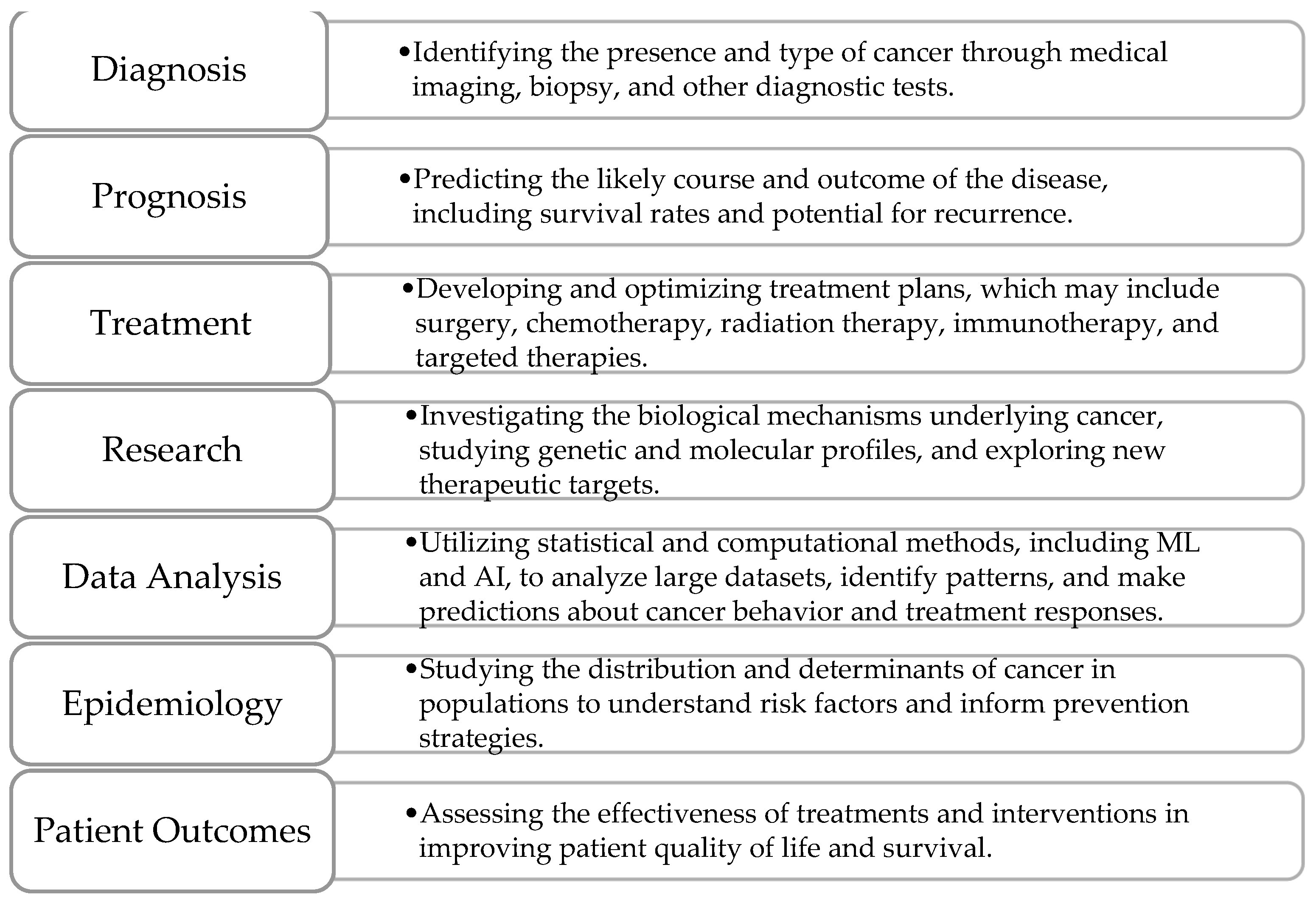
Analyzes and highlights the most important aspects of the aforementioned six cancer types.

▪

Analyzes various ML methods based on benchmark datasets and several performance evaluation metrics.

▪

Identifies the majority of datasets utilized in the reviewed papers.

▪

Outlined various research challenges, potential solutions, and opportunities for cancer analysis and care suggested for future researchers.

1.3. Summary

In the following paragraphs, a concise overview of the six cancer types discussed in this paper is provided along with the imaging modalities commonly employed for their detection and diagnosis.

▪

Lung cancer originates in the tissues of the lungs, usually in the cells lining the air passages. It is strongly associated with smoking, but can also occur in non-smokers due to other risk factors like exposure to secondhand smoke, radon, or certain chemicals. Lung cancer is one of the leading causes of cancer-related deaths worldwide, emphasizing the importance of early detection and smoking cessation efforts. It is detected primarily through chest X-rays, CT scans, and PET scans. CT scans offer high-resolution images and are particularly useful for detecting small lung nodules, while PET scans help assess the metabolic activity of suspected tumors, aiding in staging and treatment planning.

▪

Breast cancer develops in the cells of the breasts, most commonly in the ducts or lobules. It predominantly affects women, but men can also develop it, although it is much less common. This cancer is often diagnosed using mammography, ultrasound, and MRI modalities. Mammography remains the gold standard for screening, while ultrasound and MRI are utilized for further evaluation of suspicious findings, particularly in dense breast tissue.

▪

Brain cancer refers to tumors that develop within the brain or its surrounding tissues. These tumors can be benign or malignant. It is diagnosed using imaging modalities like MRI, CT scans, PET scans, and sometimes biopsy for histological confirmation. MRI is the preferred imaging modality for evaluating brain tumors due to its superior soft tissue contrast, allowing for precise localization and characterization of lesions.

▪

Cervical cancer starts in the cells lining the cervix, which is the lower part of the uterus that connects to the vagina. It is primarily caused by certain strains of human papillomavirus (HPV). Regular screening tests such as Pap smear tests, HPV DNA tests, colposcopy, and biopsy can help detect cervical cancer early, when it is most treatable.

▪

Colorectal cancer develops in the colon or rectum, typically starting as polyps on the inner lining of the colon or rectum. These polyps can become cancerous over time if not removed. Screening tests rely on various imaging modalities, including colonoscopy, sigmoidoscopy, fecal occult blood tests, and CT colonography (virtual colonoscopy). Colonoscopy is considered the gold standard for detecting colorectal polyps and cancers, allowing for both visualization and tissue biopsy during the procedure.

▪

Liver cancer arises from the cells of the liver and can either start within the liver itself (primary liver cancer) or spread to the liver from other parts of the body (secondary liver cancer). Chronic liver diseases such as hepatitis B or C infection, cirrhosis, and excessive alcohol consumption are major risk factors for primary liver cancer. Its diagnosis relies on imaging modalities such as ultrasound, CT scans, MRI, and PET scans, along with blood tests for tumor markers such as alpha-fetoprotein (AFP). These imaging techniques enable the detection of liver lesions, nodules, or masses, aiding in the diagnosis, staging, and treatment planning for liver cancer patients.

ML algorithms used for cancer detection typically follow a pattern recognition approach, where the algorithm learns patterns and features from input data to distinguish between cancerous and non-cancerous cases. Such algorithms follow a specific framework, presented in Figure 2. Each step in the framework will be detailed in following sections.

The first step involves collecting a large dataset containing features extracted from various sources such as medical imaging scans. Next, the collected data undergo preprocessing steps to clean, normalize, and standardize them for analysis. This may include removing noise, handling missing values, and scaling features to ensure consistency across the dataset. Relevant features are then extracted from the preprocessed data, depending on the type of cancer and the available input data. For medical imaging data, features may include texture, shape, intensity, or structural characteristics of tumors. The ML algorithm is trained using the labeled dataset, where each instance is associated with a binary label indicating the presence or absence of cancer. The trained model is then evaluated using separate validation datasets to assess its performance using relevant metrics that will be detailed in the upcoming section. Once the model is trained and validated, it can be used to predict the likelihood of cancer for new, unseen cases. The input data are fed into the trained model, which outputs a probability score or a binary classification indicating the presence or absence of cancer. Lastly, postprocessing steps may be applied to refine the model predictions or interpret its outputs.

1.4. Methods

The studies included in this paper focus on the application of ML techniques in cancer analysis, particularly for the diagnosis, classification, and treatment of the six most frequent cancer types: lung, breast, brain, cervical, colorectal, and liver cancers. Studies were eligible if they involved analyses of medical imaging techniques (X-rays, mammography, ultrasound, CT, MRI, PET), various AI/ML methods (e.g., deep learning, transfer learning, ensemble learning), and discussed challenges or limitations of ML in cancer care. Studies were grouped based on the cancer type and ML methodology applied. The characteristics of each study were summarized in a table that focused on the ML models used and their diagnostic performance.

A comprehensive literature search was conducted on the following databases: Web of Science, PubMed, and IEEE Xplore. Additional sources included reference lists of identified articles and conference proceedings in the fields of medical imaging and oncology. Non-English studies and reviews published before 2020 were excluded. The terms utilized in the search process were related to cancer types (“lung cancer”, “breast cancer”, etc.), ML methodologies (“deep learning”, “transfer learning”, etc.), medical imaging techniques (“CT”, “MRI”, “ultrasound”, etc.), and key areas of focus (“classification”, “segmentation”).

A single reviewer conducted the screening of titles, abstracts, and full-text articles to identify studies meeting the inclusion criteria. No automation tools were used in the selection process. The same reviewer performed the data extraction, collecting information such as study characteristics (e.g., author, year, cancer type, ML model, dataset used) and outcomes (e.g., accuracy). No formal risk-of-bias assessment was performed.

2. Medical Imaging and Diagnostic Techniques: An Overview of Key Modalities

Medical imaging techniques, together with deep learning (DL) methods, have emerged as powerful tools in the field of cancer analysis. The intersection of advanced imaging technologies and AI has led to more accurate, efficient, and early detection of cancer, revolutionizing the way healthcare professionals diagnose and treat the disease. This section briefly presents some of the key medical imaging techniques, including their underlying principles, applications, and comparative advantages when used for DL applications in cancer analysis.

2.1. X-Rays

X-rays are a type of invisible light that can pass through solid objects, including human tissue. When X-rays are directed at the body, they can create images of the inside of the body, like bones or organs, by showing how much of the X-rays are absorbed or passed through different tissues. The resulting image, typically a 2D projection, can have resolutions as fine as 100 microns, with intensities indicating X-ray absorption levels [4].

2.2. Mammography

Mammography is a specialized medical imaging technique used primarily for breast cancer screening and diagnosis [5]. It involves taking low-dose X-ray images [6] of the breast tissue to detect abnormalities such as tumors, cysts, or calcifications. These images, called mammograms, can help physicians detect early signs of breast cancer [6], such as abnormal lumps or masses, before they can be felt.

2.3. Ultrasound

Ultrasound (US) is a non-invasive and safe imaging method with extensive availability and patient comfort [7] that uses high-frequency sound waves. These waves reflect back when they hit tissues, and the returning echoes are captured to create real-time images of internal structures. The non-ionizing nature of US makes it safer for patients, as the absence of radiation reduces health risks and enhances patient comfort during diagnostic procedures. However, it fails to provide comprehensive images of organs or specific areas under examination, as its penetration capability into deeper tissues is reduced. This limitation results in incomplete images, impacting the overall visualization quality of organs, which may hinder the diagnostic accuracy and thorough assessment of certain medical conditions.

2.4. Computed Tomography

Computed tomography (CT) stands out as a fast and readily available imaging method. A CT scan is a diagnostic tool that employs X-ray images taken from various angles around the body, utilizing computer processing to generate detailed cross-sectional images (slices) of bones, blood vessels, and soft tissues. CT scan images provide superior information compared to plain X-rays, enabling a comprehensive assessment of various anatomical structures. This imaging technique allows for the identification of abnormalities in bones, blood vessels, and soft tissues, facilitating a thorough examination [8].

2.5. Positron Emission Tomography

Positron-emission tomography (PET) has transitioned from a primarily research-focused tool to an indispensable imaging modality for evaluating cancer. It uses a radioactive tracer to emit gamma rays, which are detected to create detailed images of the body’s metabolic processes. While PET offers high sensitivity for malignancy detection, its practical use as a standalone imaging modality is often limited, as it provides imprecise anatomical localization due to limited spatial resolution [9]. The advent of integrated PET–CT, a combination of PET and CT in a single device, has addressed this limitation. This approach allows for the merging of PET and CT datasets acquired during a single examination, providing both morphological and metabolic information and enhancing the accuracy and reliability of cancer staging.

2.6. Magnetic Resonance Imaging

Magnetic resonance imaging (MRI) is a precise and accurate method for tumor diagnosis, leveraging high contrasts among soft tissues in the obtained images. Although this characteristic makes it particularly effective in identifying and characterizing tumors, the diagnostic accuracy of MRI can be influenced by both patient- and operator-related factors. Patient-related considerations, such as claustrophobia, implanted materials, or devices, and uncomfortable situations, may pose limitations on the application of MRI and impact the quality of the results [10]. In contrast to CT, MRI operates without ionizing radiation, relying on magnetic stimulation of hydrogen atoms to create detailed images of targeted tissues. MRI uses powerful magnetic fields and radio waves to produce precise images of the internal structures within the body and relies on the behavior of hydrogen atoms in the body’s tissues when exposed to these magnetic fields.

2.7. Endoscopic Biopsy

Endoscopic biopsy is a procedure commonly used to obtain tissue samples from the gastrointestinal tract [11] and respiratory system [12] and involves using an endoscope, which is a long, flexible tube with a camera and light at its tip, to visualize the inside of these organs and guide the biopsy procedure. Endoscopic biopsy may be performed in various areas of the body, as presented below.

2.7.1. Colonoscopy

Colonoscopy [11,13] is a medical procedure used to examine the inside of the colon and rectum. During the procedure, if any suspicious growths or polyps are found, they can be removed or biopsied for further examination. Colonoscopy, with or without removal of a lesion, is an invasive procedure and can carry some risks, such as bleeding and perforation, although these are considered to be low.

2.7.2. Bronchoscopy

Bronchoscopy [12,14] is a medical procedure used to examine the inside of the airways and lungs. If a suspicious mass or lesion is found during the procedure, a biopsy can be taken for further examination under a microscope. The risks associated with bronchoscopy are generally considered to be low, and include bleeding, infection, and pneumothorax.

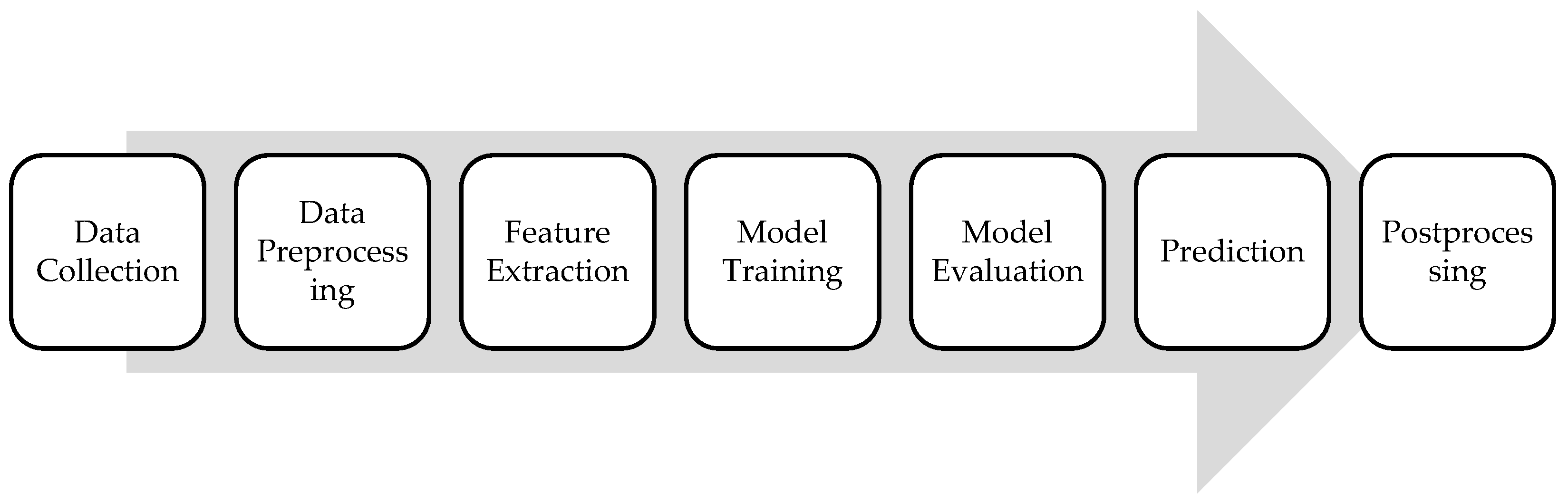
3. Machine Learning Framework

In cancer analysis, building effective ML models is crucial for accurate diagnosis, prognosis, and treatment planning. This section outlines the essential workflow stages previously presented in Figure 2: gathering data, preprocessing it for quality, extracting relevant features, training and evaluating the model, and finally, making predictions and refining outputs. Each stage plays a vital role in creating models that are accurate and robust.

3.1. Data Collection

In cancer analysis, data collection involves gathering various types of medical data, including imaging data (such as MRI, CT, or histopathology images), clinical records, genetic information, and biomarker levels. High-quality, annotated datasets are crucial, especially for tasks such as tumor classification and segmentation. Data may come from hospital databases, clinical trials, or publicly available medical repositories. It is important to collect diverse data across different patient demographics and cancer types to build a robust and generalizable model [15].

3.2. Data Preprocessing

Medical data, particularly images, require extensive preprocessing to handle noise, artifacts, and varying imaging conditions. Preprocessing steps include normalization (e.g., adjusting intensity values in images), resizing to a consistent scale, removing artifacts (e.g., motion blur in MRIs) using filters, and enhancing the contrast. For segmentation tasks, creating accurate masks that outline the tumor is vital for model training. Data augmentation techniques, such as rotation, flipping, or contrast adjustment, can help to increase the dataset’s variability and improve model robustness. Handling missing or inconsistent clinical data, such as incomplete patient records, is also part of this stage [16].

3.3. Feature Extraction

In cancer analysis, feature extraction often involves identifying key characteristics from imaging data, such as tumor size, shape, texture, and intensity patterns. Advanced methods like radiomics can quantify these features to capture the heterogeneity within a tumor. For segmentation tasks, features may include pixel intensity gradients or edge detection to outline tumor boundaries accurately. In classification, features might encompass not only image characteristics but also clinical data like patient age, genetic markers, and lab results.

3.4. Model Training

Model training in cancer analysis involves using annotated datasets (e.g., labeled images indicating tumor presence or delineated tumor regions) to teach the model to recognize cancerous patterns. For classification, algorithms like CNNs, SVMs, or ensemble methods are commonly used to differentiate between benign and malignant cases. For segmentation, more specialized architectures like U-Net are employed to accurately identify and delineate tumor regions.

Table 1. Overview of the key model training algorithms.

Algorithm	Description	Strengths	Weaknesses	Applications
SVM [18]	Finds the hyperplane that best separates the data points of different classes.	▪ Effective for smaller datasets. ▪ Performs well in high-dimensional spaces. ▪ Works well for binary classification. ▪ Can handle linear and non-linear classification using kernel tricks.	▪ Computationally expensive for large datasets. ▪ Less effective with complex image patterns or overlapping features. ▪ Difficult to interpret.	▪ Binary (e.g., benign vs. malignant) or multi-class classification. ▪ Regression.
k-NN [18]	Classifies data based on the majority class of the k-nearest neighbors in the dataset.	▪ Easy to implement. ▪ Handles noise reasonably well when imaging features are carefully preprocessed. ▪ Intuitive and interpretable.	▪ High computational cost for large datasets. ▪ Sensitive to irrelevant features and data scaling.	▪ Binary (e.g., benign vs. malignant) or multi-class classification. ▪ Used in preliminary analysis or quick tumor identification.
Decision Tree [18]	A tree-like model of decisions and their possible consequences.	▪ Easy to interpret. ▪ Works well for small datasets. ▪ Handles both categorical and numerical data.	▪ Prone to overfitting. ▪ Sensitive to noise, especially with high-dimensional imaging data.	▪ Binary or multi-class classification. ▪ Regression. ▪ Can assist in feature importance identification in tumor images.
Random Forest [18]	An EL method that builds multiple decision trees and combines them for a more accurate prediction.	▪ Reduces overfitting. ▪ Handles large datasets well. ▪ Can detect multiple feature types (e.g., color, shape, texture) across a large image dataset.	▪ Resource-intensive and slower for very high-resolution imaging. ▪ Difficult to interpret individual feature impact.	▪ Binary or multi-class classification. ▪ Regression. ▪ Helpful in feature selection for detailed tumor analysis.
Extra Trees [18]	Similar to random forest, but selects splits at random rather than calculating the best possible split, leading to faster training times.	▪ Faster training than random forest. ▪ Less prone to overfitting due to the use of random splits. ▪ Capable of extracting important diagnostic features even from noisy data.	▪ Slower and more resource-intensive for large datasets. ▪ Prone to overfitting if hyperparameters are not well-tuned. ▪ Less interpretable in terms of specific imaging feature impact.	▪ Binary or multi-class classification. ▪ Regression. ▪ Tissue differentiation, cell segmentation.
Logistic Regression [18]	Estimates the probability that a given input belongs to a particular class.	▪ Simple and easy to implement. ▪ Outputs probabilities, making predictions interpretable. ▪ Provides insight into which features contribute most to cancer presence.	▪ Can underperform with complex data without feature engineering. ▪ Limited to linearly separable data, which may be insufficient for complex cancer imaging tasks.	▪ Binary classification (e.g., benign vs. malignant).
GBM [19]	An EL method that builds models sequentially, minimizing the loss at each stage to improve accuracy.	▪ Reduces bias and variance in cancer imaging models. ▪ Flexible with hyperparameter tuning to fine-tune for complex image data. ▪ Handles non-linear relationships well.	▪ Slow to train and computationally intensive. ▪ Prone to overfitting without proper regularization. ▪ Sensitive to noisy data common in medical imaging.	▪ Binary or multi-class classification. ▪ Regression. ▪ Useful for difficult image differentiation.
XGBoost [19]	A fast and efficient implementation of GBM designed for large-scale datasets.	▪ Highly efficient. ▪ Performs well on large datasets. ▪ High performance in feature extraction for complex patterns (e.g., texture, edges).	▪ Complex and sensitive to hyperparameter tuning. ▪ Requires substantial computational resources for large-scale cancer imaging data.	▪ Binary or multi-class classification. ▪ Regression. ▪ Tumor growth prediction, feature importance in tumor identification.
Bagging [18]	An ensemble method that trains multiple models on different subsets of the data and combines their predictions to reduce variance.	▪ Reduces overfitting. ▪ Works well with noisy and high-variance data in imaging contexts. ▪ Simple and effective.	▪ Less effective on small, balanced datasets with low variance. ▪ May not provide substantial improvements on simpler imaging tasks.	▪ Binary or multi-class classification. ▪ Regression. ▪ Helpful for enhancing stability in difficult image sets.
AdaBoost [18]	A boosting algorithm that combines weak learners into a strong learner by adjusting weights to focus on harder-to-classify examples.	▪ Effective with weak learners. ▪ Can focus on ambiguous areas of cancer images where differentiation is challenging.	▪ Sensitive to noisy data in imaging, which may result in misclassification of high-variance or complex regions.	▪ Binary or multi-class classification. ▪ Suitable for refining edges or boundaries in segmentation.
Gaussian Naïve Bayes [18]	A probabilistic classifier that assumes features are normally distributed and independent of each other.	▪ Fast and simple to implement. ▪ Works well with high-dimensional data. ▪ Performs well on small datasets. ▪ Works well for preliminary screening applications or low-variance feature data.	▪ Assumes independence between features. ▪ The assumption of feature independence may not hold true in imaging, leading to inaccurate results. ▪ Prone to bias if assumptions don’t hold.	▪ Binary classification for rapid, preliminary image screening tasks.
CNN [20]	A DL algorithm primarily used for image recognition.	▪ Learns hierarchical features automatically. ▪ Handles complex image data. ▪ Excellent for identifying complex spatial relationships in tumor structure. ▪ Widely used in medical imaging analysis.	▪ Requires large annotated datasets for training. ▪ Computationally intensive, particularly with high-resolution medical images. ▪ Black-box model, harder to interpret.	▪ Binary or multi-class classification. ▪ Segmentation (e.g., organs, tumors). ▪ Object detection (e.g., organs, tumors).
VGG-16 [21]	A CNN architecture with 16 layers known for using small convolutional filters (3 × 3) and deep layers.	▪ Strong performance in identifying fine-grained cancer features. ▪ Simple yet effective deep structure. ▪ Performs well with TL.	▪ Memory-intensive and computationally expensive. ▪ Limited interpretability in context of specific image features.	▪ Binary or multi-class classification. ▪ Object detection (e.g., organs, tumors).
U-Net [22]	A type of CNN tailored for biomedical image segmentation that uses an encoder–decoder structure.	▪ Ideal for precise medical image segmentation. ▪ Handles small datasets well with data augmentation. ▪ Widely used in cancer imaging.	▪ High computational cost. ▪ Sensitive to tuning. ▪ Performance depends on high-quality annotations, which can be challenging in cancer imaging.	▪ Tumor boundary segmentation. ▪ Highly effective for delineating cancerous tissues from surrounding structures.
ResNet [23]	A DNN that introduces “residual connections” to solve the vanishing gradient problem, allowing the training of much deeper networks.	▪ Solves vanishing gradient problem. ▪ Ideal for training on very deep networks with high-dimensional cancer imaging data. ▪ Retains high accuracy without overfitting.	▪ Computationally expensive. ▪ Requires significant memory and processing power for large image datasets. ▪ More complex to train and tune.	▪ Binary or multi-class classification. ▪ Segmentation in complex cancer imaging. ▪ Object detection.

summarizes some of the most common algorithms utilized for model training in cancer analysis [17].

3.5. Model Evaluation

In medical applications, false negatives (missing a cancerous region) can have serious implications, so the evaluation must be thorough to ensure reliable clinical performance. The evaluation metrics for the performance of an ML algorithm can be categorized based on the task at hand, whether it is classification or segmentation. The following subsections will delve into the specifics of each.

3.5.1. Classification

In ML classification tasks, several performance metrics are used to evaluate the effectiveness of a classifier, typically derived from a confusion matrix [24], which is a means to evaluate the performance of a classification model by presenting a summary of the model’s predictions compared to the actual labels in a tabular format, as presented in Figure 3, where:

▪

True Positives (TP): Instances that are correctly predicted as belonging to the positive class.

▪

False Positives (FP): Instances that are incorrectly predicted as belonging to the positive class when they actually belong to the negative class.

▪

True Negatives (TN): Instances that are correctly predicted as belonging to the negative class.

▪

False Negatives (FN): Instances that are incorrectly predicted as belonging to the negative class when they actually belong to the positive class.

The most widely used performance metrics for classification problems are accuracy, precision, recall, specificity, sensitivity, F1 score, PR curve, AUC-PR curve, ROC curve, and AUC-ROC curve, which are described below [24,25].

▪

Accuracy measures the proportion of correctly classified instances out of the total instances and is calculated as the number of true positives and true negatives divided by the total number of instances:

$$Accuracy={\displaystyle \frac{TP+TN}{TP+TN+FN+FP}}$$

▪

Precision measures the proportion of true positive predictions among all positive predictions made by the classifier and is calculated as the number of true positives divided by the total number of instances predicted as positive:

$$Precision={\displaystyle \frac{TP}{TP+FP}}$$

▪

Recall or sensitivity measures the proportion of true positives that are correctly identified by the classifier and is calculated as the number of true positives divided by the total number of actual positive instances:

$$Recall (Sensitivity)={\displaystyle \frac{TP}{TP+FN}}$$

▪

Specificity measures the proportion of true negatives that are correctly identified by the classifier and is calculated as the number of true negatives divided by the total number of actual negative instances:

$$Specificity={\displaystyle \frac{TN}{TN+FP}}$$

▪

F1 score is the harmonic mean of precision and recall, providing a balance between the two metrics and is calculated as the harmonic mean of precision and recall:

$$F1\text{-}score={\displaystyle \frac{2\times Precision\times Recall}{Precision+Recall}}$$

▪

Precision–recall (PR) curves plot the precision against the recall for different threshold values used by the classifier to make predictions. Each point on the curve corresponds to a different threshold setting used by the classifier, where a higher threshold leads to higher precision but lower recall, and vice versa.

▪

Area under the PR (AUC-PR) curves summarize the performance of the classifier across all possible threshold values, with a higher AUC-PR indicating better overall performance in terms of both precision and recall.

▪

Receiver operating characteristic (ROC) curves plot the recall against the false-positive rate (FPR, which measures the proportion of false-positive predictions among all actual negative instances) for various threshold values used by the classifier to make predictions. Each point on the curve corresponds to a different threshold setting used by the classifier, where a higher threshold leads to higher specificity but lower recall, and vice versa.

▪

Area under the ROC curve (AUC-ROC or simply AUC) summarizes the performance of the classifier across all possible threshold values, with a higher AUC indicating better overall performance in terms of both recall and specificity.

3.5.2. Segmentation

In ML segmentation tasks, key metrics include the following [25,26,27].

▪

Intersection over union (IOU) measures the overlap between the predicted and ground-truth masks by calculating the ratio of the intersection to the union of the two masks:

$$IoU={\displaystyle \frac{TP}{TP+FP+FN}} or \mathrm{I}\mathrm{o}\mathrm{U}={\displaystyle \frac{\left|\mathrm{A}\bigcap \mathrm{B}\right|}{\left|\mathrm{A}\bigcup \mathrm{B}\right|}}, where:$$

$$\mathrm{A}=the predicted segmentation mask$$

$$\mathrm{B}=the ground-truth mask$$

$$\left|\mathrm{A}\bigcap \mathrm{B}\right|=the number of overlapping pixels$$

$$\left|\mathrm{A}\bigcup \mathrm{B}\right|=the total number of unique pixels in both masks$$

▪

Dice similarity coefficient (DSC) measures the spatial overlap between the predicted segmentation mask and the ground-truth mask and is calculated as twice the intersection of the predicted and ground-truth masks divided by the sum of their volumes:

$$Dice={\displaystyle \frac{2\times TP}{2\times TP+FP+FN}}={\displaystyle \frac{2\times IoU}{1+IoU}} \mathrm{o}\mathrm{r}:$$

$$Dice={\displaystyle \frac{2\times \left|A\bigcap B\right|}{\left|A\right|+\left|B\right|}}, \mathrm{w}\mathrm{h}\mathrm{e}\mathrm{r}\mathrm{e}$$

$$\mathrm{A}=\mathrm{t}\mathrm{h}\mathrm{e} \mathrm{p}\mathrm{r}\mathrm{e}\mathrm{d}\mathrm{i}\mathrm{c}\mathrm{t}\mathrm{e}\mathrm{d} \mathrm{s}\mathrm{e}\mathrm{g}\mathrm{m}\mathrm{e}\mathrm{n}\mathrm{t}\mathrm{a}\mathrm{t}\mathrm{i}\mathrm{o}\mathrm{n} \mathrm{m}\mathrm{a}\mathrm{s}\mathrm{k}$$

$$\mathrm{B}=\mathrm{t}\mathrm{h}\mathrm{e} \mathrm{g}\mathrm{r}\mathrm{o}\mathrm{u}\mathrm{n}\mathrm{d}-\mathrm{t}\mathrm{r}\mathrm{u}\mathrm{t}\mathrm{h} \mathrm{m}\mathrm{a}\mathrm{s}\mathrm{k}$$

$$\left|\mathrm{A}\bigcap \mathrm{B}\right|=\mathrm{t}\mathrm{h}\mathrm{e} \mathrm{n}\mathrm{u}\mathrm{m}\mathrm{b}\mathrm{e}\mathrm{r} \mathrm{o}\mathrm{f} \mathrm{o}\mathrm{v}\mathrm{e}\mathrm{r} \mathrm{l}\mathrm{a}\mathrm{p}\mathrm{p}\mathrm{i}\mathrm{n}\mathrm{g} \mathrm{p}\mathrm{i}\mathrm{x}\mathrm{e}\mathrm{l}\mathrm{s}$$

$$\left|A\right|=\mathrm{t}\mathrm{h}\mathrm{e} \mathrm{t}\mathrm{o}\mathrm{t}\mathrm{a}\mathrm{l} \mathrm{n}\mathrm{u}\mathrm{m}\mathrm{b}\mathrm{e}\mathrm{r} \mathrm{o}\mathrm{f} \mathrm{p}\mathrm{i}\mathrm{x}\mathrm{e}\mathrm{l}\mathrm{s} \mathrm{i}\mathrm{n} \mathrm{t}\mathrm{h}\mathrm{e} \mathrm{p}\mathrm{r}\mathrm{e}\mathrm{d}\mathrm{i}\mathrm{c}\mathrm{t}\mathrm{e}\mathrm{d} \mathrm{m}\mathrm{a}\mathrm{s}\mathrm{k}$$

$$\left|B\right|=\mathrm{t}\mathrm{h}\mathrm{e} \mathrm{t}\mathrm{o}\mathrm{t}\mathrm{a}\mathrm{l} \mathrm{n}\mathrm{u}\mathrm{m}\mathrm{b}\mathrm{e}\mathrm{r} \mathrm{o}\mathrm{f} \mathrm{p}\mathrm{i}\mathrm{x}\mathrm{e}\mathrm{l}\mathrm{s} \mathrm{i}\mathrm{n} \mathrm{t}\mathrm{h}\mathrm{e} \mathrm{g}\mathrm{r}\mathrm{o}\mathrm{u}\mathrm{n}\mathrm{d}-\mathrm{t}\mathrm{r}\mathrm{u}\mathrm{t}\mathrm{h} \mathrm{m}\mathrm{a}\mathrm{s}\mathrm{k}$$

▪

Mean intersection over union (mIoU) measures the average IoU across all classes or segments in the image:

$$mIoU={\displaystyle \frac{1}{N}}{\sum }_{i=1}^N{IoU}_i, \mathrm{w}\mathrm{h}\mathrm{e}\mathrm{r}\mathrm{e}:$$

$$\mathrm{N}=\mathrm{t}\mathrm{h}\mathrm{e} \mathrm{n}\mathrm{u}\mathrm{m}\mathrm{b}\mathrm{e}\mathrm{r} \mathrm{o}\mathrm{f} \mathrm{c}\mathrm{l}\mathrm{a}\mathrm{s}\mathrm{s}\mathrm{e}\mathrm{s}$$

$${\mathrm{I}\mathrm{o}\mathrm{U}}_{\mathrm{i}}=\mathrm{t}\mathrm{h}\mathrm{e} \mathrm{I}\mathrm{o}\mathrm{U} \mathrm{f}\mathrm{o}\mathrm{r} \mathrm{e}\mathrm{a}\mathrm{c}\mathrm{h} \mathrm{c}\mathrm{l}\mathrm{a}\mathrm{s}\mathrm{s} \mathrm{i}$$

▪

Pixel accuracy measures the proportion of correctly classified pixels in the segmentation mask and is calculated as the number of pixels correctly classified divided by the total number of pixels in the image:

$$Pixel Accuracy={\displaystyle \frac{Number of correctly classified pixels}{Total number of pixels}}$$

▪

Mean average precision (mAP) summarizes the precision–recall (PR) curve across multiple classes or categories and is calculated in three steps:

• For each class or category in the dataset, the PR curve is computed based on the model’s predictions and ground-truth annotations.
• The AUC-AP curve is computed for each class.
• The mAP is calculated by taking the mean of the average precision values across all classes in the dataset.

$$mAP={\displaystyle \frac{1}{N}}{\sum }_{i=1}^N{AP}_i, \mathrm{w}\mathrm{h}\mathrm{e}\mathrm{r}\mathrm{e}:$$

$$\mathrm{C}=\mathrm{t}\mathrm{h}\mathrm{e} \mathrm{t}\mathrm{o}\mathrm{t}\mathrm{a}\mathrm{l} \mathrm{n}\mathrm{u}\mathrm{m}\mathrm{b}\mathrm{e}\mathrm{r} \mathrm{o}\mathrm{f} \mathrm{c}\mathrm{l}\mathrm{a}\mathrm{s}\mathrm{s}\mathrm{e}\mathrm{s} \mathrm{i}\mathrm{n} \mathrm{t}\mathrm{h}\mathrm{e} \mathrm{d}\mathrm{a}\mathrm{t}\mathrm{a}\mathrm{s}\mathrm{e}\mathrm{t}$$

$${\mathrm{A}\mathrm{P}}_{\mathrm{i}}=\mathrm{t}\mathrm{h}\mathrm{e} \mathrm{a}\mathrm{v}\mathrm{e}\mathrm{r}\mathrm{a}\mathrm{g}\mathrm{e} \mathrm{p}\mathrm{r}\mathrm{e}\mathrm{c}\mathrm{i}\mathrm{s}\mathrm{i}\mathrm{o}\mathrm{n} \mathrm{f}\mathrm{o}\mathrm{r} \mathrm{c}\mathrm{l}\mathrm{a}\mathrm{s}\mathrm{s} \mathrm{i}$$

▪

Hausdorff distance (HD) measures the similarity between two sets of points in a metric space. It quantifies the maximum distance from a point in one set to the closest point in the other set, and vice versa.

The directed Hausdorff distance from set A to set B is defined as:

$$h\left(A,B\right)={max}_{a\in A}{min}_{b\in B}d\left(a,b\right), \mathrm{w}\mathrm{h}\mathrm{e}\mathrm{r}\mathrm{e}:$$

$$\mathrm{d}\left(\mathrm{a},\mathrm{b}\right)=\mathrm{t}\mathrm{h}\mathrm{e} \mathrm{d}\mathrm{i}\mathrm{s}\mathrm{t}\mathrm{a}\mathrm{n}\mathrm{c}\mathrm{e} \mathrm{b}\mathrm{e}\mathrm{t}\mathrm{w}\mathrm{e}\mathrm{e}\mathrm{n} \mathrm{p}\mathrm{o}\mathrm{i}\mathrm{n}\mathrm{t}\mathrm{s} \mathrm{a} \mathrm{a}\mathrm{n}\mathrm{d} \mathrm{b} (\mathrm{w}\mathrm{h}\mathrm{e}\mathrm{r}\mathrm{e} \mathrm{a}\in \mathrm{A} \mathrm{a}\mathrm{n}\mathrm{d} \mathrm{b}\in \mathrm{B})$$

Similarly, the directed Hausdorff distance from set B to set A is defined as:

$$h\left(B,A\right)={max}_{b\in B}{min}_{a\in A}d\left(b,a\right)$$

The Hausdorff distance between sets A and B is therefore defined as the maximum of the directed Hausdorff distances:

$$H\left(A,B\right)=\mathit{max} (h\left(A,b\right),h(B,A\left)\right)$$

3.6. Prediction

Once trained and evaluated, the model is deployed to predict cancer presence or segment tumors in new, unseen patient data. The same algorithms used for model training are employed to take in new input data, apply the patterns and parameters learned during training, and output predictions. In general, for classification, the model outputs a probability score indicating the likelihood of cancer, which can aid in early diagnosis, while for segmentation tasks, the model provides a pixel-wise mask outlining the tumor boundaries, assisting radiologists and oncologists in treatment planning.

3.7. Postprocessing

Postprocessing is essential to refine the model’s output into clinically actionable insights. In segmentation, postprocessing might involve smoothing tumor boundaries, removing noise, or filling gaps in the predicted mask to improve visual clarity. For classification, probability scores might be converted into binary labels (cancerous or non-cancerous) based on a decision threshold. Additionally, postprocessing can include combining predictions with other clinical data, generating reports, or highlighting regions of interest on images for further review by medical experts.

A critical aspect of postprocessing in cancer analysis is model interpretability. After an ML model has made its predictions, interpretability techniques can be applied to explain the reasoning behind those predictions. These interpretability methods provide crucial insights, especially in medical applications, where understanding how and why the model arrived at a specific decision is essential for gaining clinical trust and ensuring the transparency of the model. Commonly used interpretability methods include:

▪

Shapley additive explanation (SHAP) [28] values explain individual predictions by attributing the contribution of each feature (e.g., patient characteristics or image pixels) to the final outcome. SHAP helps clinicians understand which variables had the most significant influence on the prediction.

▪

Local interpretable model-agnostic explanations (LIME) [29] approximate complex models by perturbing input data slightly and analyzing the effect on predictions. It provides local explanations for individual instances, making it particularly useful in understanding predictions made by complex, black-box models.

▪

Gradient-weighted class activation mapping (Grad-CAM) [30] generates visual explanations of model decisions by highlighting the regions of an image that were most influential in the model’s decision-making process. This is particularly important in cancer imaging, where clinicians need to verify that the model is focusing on relevant areas when diagnosing or classifying cancer.

▪

Score-weighted class activation mapping (Score-CAM) [31] provides visual explanations for the decisions made by CNNs, particularly in image classification and object detection tasks. It extends the concept of Grad-CAM by using the activation maps directly from the network to generate class-specific attention maps, but without relying on the gradients.

4. Literature Review

This section provides an in-depth analysis of existing research and developments in the field of ML-based cancer analysis, with a specific focus on the most prevalent and deadly six types of cancer: lung, breast, brain, cervical, colorectal, and liver cancers. These specific types of cancer are associated with high mortality rates and are frequently diagnosed at advanced stages. Recent research has demonstrated that early detection plays a crucial role in reducing mortality rates and improving patient survival rates. A notable trend observed in recent years is the extensive research efforts dedicated to the detection and diagnosis of these cancers utilizing ML-based techniques. This section aims to review the current state of the art, methodologies, and advancements in utilizing ML techniques for the diagnosis, prognosis, and treatment of these selected cancers. By examining a wide range of studies and approaches within these specific cancer types, this review offers insights into the various ML algorithms, data sources, and evaluation methods used in cancer analysis.

4.1. Lung Cancer

Lung cancer accounts for approximately 14% of the annual new cancer cases in the United States, surpassing the combined deaths caused by breast, prostate, and colon cancers [32]. Early-stage lung cancer typically lacks symptoms, leading to late-stage diagnoses. The 5-year survival rate for locally detected lung cancers is 55%, but most patients receive diagnoses at advanced stages, resulting in significantly lower survival rates (overall 5-year survival rate of 18%) [33]. The utilization of ML has the potential to revolutionize the early detection of lung cancer, leading to enhanced accuracy in results and more targeted treatment approaches, which could substantially increase patient survival rates.

Jassim et al. [34] present a transfer DL ensemble model for predicting lung cancer using CT images. The Chest CT-Scan images dataset [35] comprises 1000 CT images across four classes relevant to lung cancer. The classes include adenocarcinoma, large cell carcinoma, squamous cell carcinoma, and normal tissue. The model leverages the capabilities of three ImageNet dataset pre-trained DL architectures, namely, EfficientNetB3, ResNet50, and ResNet101, with TL and applied data augmentation techniques for training. These models are further trained on the lung cancer dataset to fine-tune the weights for specific features relevant to lung cancer classification. Each model configuration includes modifications specific to lung cancer imaging, such as adjustments in layer depths and learning rates. EfficientNetB3 emerged as the top-performing model, displaying the most effective convergence with average precision of 94%, recall of 93%, and F1 score of 93%. In comparison, the ResNet50 model achieved precision, recall, and F1 score values of 88%, 81%, and 81%, respectively, while the ResNet101 model achieved values of 94%, 93%, and 93%, respectively. The maximum accuracy achieved by the models presented in this paper is 99.44%.

Muhtasim et al. [36] propose a multi-classification approach for detecting lung nodules using AI on CT scan images from the IQ-OTHNCCD lung cancer dataset [37], consisting of 1190 CT scan images classified into normal, benign, and malignant. It employs TL with the VGG16 model and morphological segmentation to enhance the accuracy and computational efficiency of lung cancer detection. Morphological operations are applied to segment the region of interest and extract distinct morphological features. The classification task implements a DL architecture combined with seven different ML algorithms, namely, decision tree, k-NN, random forest, extra trees, extreme gradient boosting, SVM, and logistic regression, to classify lung nodules into malignant, benign, and normal categories. The proposed stacked ensemble model combines the CNN with the VGG16 TL model to achieve accuracy, precision, recall, and F1 score of 99.55%, 0.996, 0.995, and 0.995, respectively.

Luo [38] introduces the LLC-QE model, an innovative approach combining EL and reinforcement learning to improve lung cancer classification. The model classifies lung cancer into four classes: adenocarcinoma, squamous cell carcinoma, large-cell carcinoma, and small-cell carcinoma. The study utilizes the LIDC-IDRI dataset [39] comprising 1018 CT scans, primarily composed of non-cancer cases, to train and validate the model. To address dataset imbalances, the training employs strategies that involve differential reward systems in reinforcement learning, focusing on underrepresented classes to improve model sensitivity to less frequent cases. The artificial bee colony algorithm is used during pre-training to enhance the initialization of network weights, and a series of CNNs act as feature extractors. The reinforcement learning mechanism views image classification as a series of decisions made by the network within a Markov decision process framework and adopts a nuanced reward system where correct classifications of minority classes receive higher rewards compared to majority classes, encouraging the model to pay more attention to the harder-to-detect instances. The features extracted by individual CNNs are then merged to harness the collective power of multiple models, resulting in an average classification accuracy of 92.9%.

Mamun et al. [40] assess the effectiveness of various EL techniques in binary classifying lung cancer using the Lung Cancer dataset [41] from Kaggle, containing 309 instances with 16 attributes. These attributes included various symptoms and patient characteristics, such as age, smoking status, chronic disease, alcohol consumption, coughing, shortness of breath, and chest pain. The ensemble methods applied include XGBoost, LightGBM, Bagging, and AdaBoost. The data underwent preprocessing to handle missing values and balance the dataset using the synthetic minority over-sampling technique (SMOTE). The models were evaluated based on accuracy, precision, recall, F1 score, and AUC. XGBoost performed the best among the tested models, achieving accuracy of 94.42%, precision of 95.66%, and AUC of 98.14%, highlighting its capability in handling imbalanced and complex datasets. The LightGBM, AdaBoost, and Bagging methods achieved accuracy values of 92.55%, 90.70%, and 89.76%, respectively.

Venkatesh and Raamesh [42] examine the application of EL techniques for predicting lung cancer survivability through binary classification methods using the Surveillance, Epidemiology, and End Results (SEER) dataset [43]. The study evaluates the effectiveness of bagging and AdaBoost ensemble methods combined with k-NN, decision tree, and neural network classifiers. The dataset consists of 1000 samples with 149 attributes initially, which was reduced to 24 attributes after preprocessing, including smoking, gender, air pollution, chronic lung disease, chest pain, wheezing, dry cough, snoring, and swallowing difficulty. The previously mentioned ensemble techniques are used to improve the predictive performance by reducing variance (bagging) and bias (AdaBoost), as well as improving the accuracy of weak classifiers. The outputs from the different models are combined using a systematic voting mechanism to finalize the survival prediction. The results indicate that both bagging and AdaBoost techniques improve the performance of individual models. Specifically, the accuracy scores for decision trees with bagging and AdaBoost were 0.973 and 0.982, respectively, for k-NN, bagging and AdaBoost achieved scores of 0.932 and 0.951, and for neural networks, bagging and AdaBoost attained scores of 0.912 and 0.931. The integrated model achieved an accuracy score of 0.983, surpassing the scores of individual algorithms both with and without ensemble methods.

Said et al. [44] present a system for lung cancer diagnosis using segmentation and binary classification techniques based on DL architectures, specifically utilizing UNETR for segmentation and a self-supervised network for classification. The Decathlon dataset [45], consisting of 96 3D CT scan volumes, is utilized for training and testing. The segmentation part employs the UNETR neural network, a combination of U-Net and transformers, to achieve an DSC of 96.42%. The classification part uses a self-supervised neural network to classify segmented nodules as either benign or malignant, achieving a classification accuracy of 98.77%.

Table 2. Summary of Lung Cancer studies.

Author	Model	Data Type	Dataset		Preprocessing
			Size	Classes
Jassim et al. [34]	Transfer DL Ensemble	CT	1000	Normal Adenocarcinoma Large cell Squamous cell	Conversion to RGB Resizing Data augmentation
Muhtasim et al. [36]	Ensemble CNN + VGG16 TL	CT	1190	Normal Benign Malignant	Resizing Normalization Smoothing Enhancement Morphological segmentation
Luo [38]	LLC-QE	CT	1018	Non-nodule > or =3 mm Nodule > or =3 mm Nodule < 3 mm	-
Mamun et al. [40]	XGBoost LightGBM AdaBoost Bagging	16 attributes	309	Normal Cancer	Feature extraction Data cleaning Missing value handling Categorical variables transformation SMOTE
Venkatesh & Raamesh [42]	Bagging AdaBoost Integrated	24 attributes	1000	Normal Cancer	Interpolation Normalization
Said et al. [44]	UNETR	CT	96	Benign Malignant	Segmentation

provides an overview of lung cancer studies, including model name, dataset details, and preprocessing methods. No interpretability methods were presented in of any these papers.

4.2. Breast Cancer

Breast cancer is a common type of cancer among women, accounting for approximately 30% of all annual new cancer cases among women [46]. Globally, there were 2.3 million women (11.6% of the total new cases of cancer) diagnosed with breast cancer and 670,000 deaths (6.9% of the total cancer deaths) attributed to the disease in 2022 [47]. Early detection through screening mammography can decrease breast cancer mortality by up to 20% [48]. Breast US faces challenges due to image complexity, including noise, artifacts, and low contrast. Manual analysis by sonographers is time-consuming, subjective, and can result in unintended misdiagnoses due to fatigue. Therefore, the integration of computer-aided detection or AI is crucial for enhancing the accuracy of screening breast US, reducing both false positives and false negatives, and minimizing unnecessary biopsies [49].

Interlenghi et al. [50] developed a radiomics-based ML binary classification model that predicts the BI-RADS category of suspicious breast lesions detected through US with an accuracy of approximately 92%. A dataset of 821 images, comprising 834 suspicious breast masses from 819 patients, was collected retrospectively from US-guided core needle biopsies performed by four certified breast radiologists using six different US systems. The dataset consists of 404 malignant and 430 benign lesions based on histopathology. A balanced image set of biopsy-proven benign and malignant lesions (299 each) is used to train and cross-validate ensembles of ML algorithms supervised by histopathological diagnosis. An ensemble of SVMs, using a majority vote, demonstrated the ability to reduce the biopsy rate of benign lesions by 15% to 18% while maintaining a sensitivity of over 94% in external testing. This model was tested on two additional image sets, resulting in positive predictive values (PPV) of 45.9% and 50.5% and sensitivity of 98.0% and 94.4%, respectively, outperforming the radiologists’ PPVs. The model achieved low error rates in assigning BI-RADS categories, and the radiologists accepted the model’s classifications for most masses, indicating instances where the model performed better than the radiologists by assigning a more accurate BI-RADS classification.

Kavitha et al. [51] propose a novel optimal multi-level thresholding-based segmentation with DL-enabled capsule network (OMLTS-DLCN) model for breast cancer diagnosis and multi-class classification. The model incorporates an adaptive fuzzy-based median filtering procedure to eliminate noise. The segmentation technique employed is the optimal Kapur’s multilevel thresholding with shell game optimization (OKMT-SGO) algorithm, which effectively detects the diseased portion in mammogram images. Feature extraction is performed using the CapsNet model, and the final classification is achieved using the backpropagation neural network (BPNN) model, determining appropriate class labels. The performance evaluation on the Mini-MIAS [52] (322 images) and CBIS-DDSM [53] (13,128 images) datasets, containing normal, benign, and malignant classes, demonstrates that the presented OMLTS-DLCN model outperforms other methods in terms of classification accuracy, with an accuracy of 98.50% and 97.56%, respectively.

Chen et al. [54] introduce a novel approach called DSEU-Net (squeeze-and-excitation (SE) attention U-Net with deep supervision) for the segmentation of medical US images. The proposed method combines several key elements to enhance the accuracy and robustness of the segmentation process. Firstly, a deeper U-Net architecture is employed as a benchmark network to effectively capture the intricate features present in complex US images. Next, the SE block is integrated as a bridge between the encoder and decoder, allowing for enhanced attention on relevant object regions. The SE block not only strengthens the connections between distant but useful information but also suppresses the introduction of irrelevant information, improving the overall segmentation quality. Furthermore, deep supervised constraints are incorporated into the decoding stage of the network to refine the prediction masks of US images, which further improves the accuracy and reliability of the segmentation results. The performance of DSEU-Net in US image segmentation was evaluated using extensive experiments on two clinical US breast datasets. Specifically, when applied to the first dataset (BUSI [55]), DSEU-Net achieved IOU, precision, recall, specificity, DSC, and accuracy values of 70.36%, 79.73%, 82.70%, 97.42%, 78.51%, and 95.81%, respectively. Similarly, for the second dataset, the method achieved Jaccard coefficient, precision, recall, specificity, and DSC values of 73.17%, 82.58%, 84.02%, 99.05%, and 81.50%, respectively. These results demonstrate the significant improvement of DSEU-Net over the original U-Net, with an average increase of 8.28% and 12.55% on the five-evaluation metrics for the two breast US datasets.

Dogiwal’s paper [56] investigates the effectiveness of supervised ML techniques in predicting breast cancer using histopathological data. The dataset used in this study was sourced from the UCI Machine Learning Repository, specifically the Breast Cancer Wisconsin (Diagnostic) dataset [57], which consists of 699 samples with 458 benign (65.5%) and 241 malignant (34.5%) instances with 32 attributes. This study utilizes PCA to reduce the number of dimensions while preserving the most significant information. The approach also involves feature engineering to enhance model performance by selecting the most relevant features. The study focuses on the application of three prominent algorithms, namely, random forest, logistic regression, and SVM, for breast cancer binary classification. The random forest algorithm achieved an accuracy of 98.6%, with precision and recall scores of 0.99 and 0.98, respectively. In comparison, the logistic regression algorithm attained an accuracy of 94.41%, with precision and recall scores both at 0.94. Similarly, the SVM algorithm yielded an accuracy of 93.71%, with precision and recall scores also at 0.93.

Al-Azzam and Shatnawi’s study [58] evaluates the effectiveness of both SL and semi-SL algorithms in diagnosing breast cancer using the Breast Cancer Wisconsin (Diagnostic) dataset [57], containing 569 instances with 30 features extracted from digital images of fine needle-aspirates (FNAs) of breast masses. The dataset is split into training (80%) and testing (20%) sets for both approaches, noting that for the semi-SL algorithm, the training data was divided into 50% labeled data and 50% unlabeled data. Several models, such as logistic regression, Gaussian naïve Bayes, SVM (both linear and RBF), decision tree, random forest, XGBoost, GBM, and k-NN, are trained using the labeled dataset for both approaches. All algorithms demonstrated strong performance on the test data, a minimal disparity in accuracy between the SL and semi-SL techniques being observed. Results showed that logistic regression (SL = 97%, SSL = 98%) and k-NN (SL = 98%, SSL = 97%) achieved the highest accuracy for classifying malignant and benign tumors.

Ayana et al. [59] explore a novel multistage TL (MSTL) approach tailored for US breast cancer image binary classification. The dataset consists of 20,400 cancer cell line microscopic images and US images from two datasets: Mendeley [60] (200 images) and MT-Small-Dataset [55,61] (400 images). The presented TL approach begins with a pre-trained model on ImageNet, adapted to cancer cell line microscopic images. This stage involves fine-tuning the model to recognize features relevant to medical contexts, particularly those that are morphologically similar to features in US images. Then, it uses the tuned model as a base to further train on US breast cancer images. This two-step process allows the model to refine its ability to differentiate between malignant and benign features with higher accuracy. The study employs three different CNN models: EfficientNetB2, InceptionV3, and ResNet50. The best performance was achieved using the ResNet50 with the Adagrad optimizer, resulting in a test accuracy of 99.0% on the Mendeley dataset and 98.7% on the MT-Small-Dataset.

Umer et al. [61] propose an innovative approach for breast cancer binary classification using a combination of convoluted features extracted through DL techniques and an ensemble of ML algorithms. The study employs a custom CNN model designed to extract deep convoluted features from mammographic images from the Breast Cancer Wisconsin (Diagnostic) dataset [57] consisting of 32 features. After feature extraction, multiple ML algorithms, such as random forest, decision trees, SVM, and k-NN, are employed to classify the images into benign or malignant. The final classification is determined through a majority voting system where each algorithm contributes equally to the decision-making process. The dataset was split into 70% training and 30% testing. This ensemble approach reduces the likelihood of misclassification by leveraging the diverse strengths of different algorithms, reaching accuracy of 99.89%, precision of 99.89%, recall of 99.92%, and F1 score of 99.90%.

The study conducted by Hekal et al. [62] proposes an ensemble DL system designed for binary classification of breast cancer. The system processes suspected nodule regions (SNRs) extracted from mammogram images, utilizing four different TL CNNs and subsequent binary SVM classifiers. The study uses the CBIS-DDSM [53] dataset, which provides 3549 region-of-interest (ROI) images with both mass and calcification cases containing annotations for both malignant and benign findings. SNRs are extracted from ROI images using an optimal dynamic thresholding method specifically tailored to adjust the threshold based on the detailed characteristics of each image. Four CNN architectures, namely, AlexNet, DenseNet-201, ResNet-50, and ResNet-101, are used and followed by a binary SVM classifier that determines if the processed SNRs are malignant or benign. The outputs from each CNN-SVM pipeline are combined using a first-order momentum method, which considers the training accuracies of the individual models. This fusion approach is designed to enhance decision-making by weighting the contribution of each model based on its performance. The proposed ensemble DL system achieved an accuracy of 94% for distinguishing benign and malignant cases and 95% for distinguishing between benign and malignant masses.

Deb et al. [63] provide a detailed analysis of segmenting mammogram images using DL architectures, specifically U-Net and BCDU-Net, which is an advanced variant of U-Net that incorporates bidirectional ConvLSTM and densely connected convolutional blocks. The INBreast dataset [64] is utilized, comprising 410 mammograms from 115 patients. Initial experiments are conducted on full mammograms to segment regions indicative of potential masses. Further experiments focus on ROIs extracted from mammograms, where the network segments smaller, more focused areas. Both U-Net and BCDU-Net are evaluated on their ability to segment whole mammograms and ROIs. The models achieved a DSC of 0.8376 and IOU of 0.7872 for the full mammogram, while for the ROI segmentation, they reported a DSC of 0.8723 and IOU of 0.8098. The study concludes that BCDU-Net provides better segmentation results, especially when focusing on ROIs.

Haris et al. [65] introduce a novel approach for breast cancer segmentation using a combination of Harris hawks optimization (HHO) with cuckoo search (CS) and an SVM classifier that aims to optimize segmentation by fine-tuning hyperparameters for enhanced accuracy in mammographic image analysis. The study utilizes the CBIS-DDSM [40] dataset. The hybrid model starts with initializing a population of hawks in the image matrix, where each hawk represents a potential solution. The fitness of each hawk is evaluated based on pixel intensity and neighboring intensities. This evaluation guides the optimization process, focusing on improving segmentation accuracy. The hybrid approach leverages the strengths of both HHO and CS, enabling a dynamic adjustment between exploration and exploitation phases, ultimately fine-tuning SVM parameters for optimal segmentation. The study concludes that the integration of HHO and CS with SVM significantly improves breast cancer segmentation in mammographic images, demonstrating an accuracy of 98.93%, a DSC of 98.77%, and an IOU of 97.68%.

Table 3. Summary of breast cancer studies.

Author	Model	Data Type	Dataset		Preprocessing
			Size	Classes
Interlenghi et al. [50]	Radiomics-based ML	US	821	Benign Malignant	Image balancing Histogram equalization
Kavitha et al. [51]	OMLTS-DLCN	Mammogram	322 + 13,128	Normal Benign Malignant	Noise reduction Thresholding Segmentation
Chen et al. [54]	DSEU-Net	US	780	Normal Benign Malignant	-
Dogiwal [56]	Random Forest Logistic Regression SVM	32 attributes	699	Benign Malignant	Feature extraction Feature selection
Al-Azzam & Shatnawi [58]	SL Semi-SL	32 features	569	Benign Malignant	Exploratory Data Analysis Correlation analysis
Ayana et al. [59]	ResNet50	US	200 + 400	Benign Malignant	Adaptive thresholding Noise reduction Data augmentation
Umer et al. [61]	Voting CNN	32 features	-	Benign Malignant	Feature extraction Label encoder
Hekal et al. [62]	Ensemble DL SVM	Mammogram	3549	Benign Malignant	ROI extraction Smoothing Otsu thresholding
Deb et al. [63]	BCDU-Net	Mammogram	410	Masses Calcifications Asymmetries Distortions	ROI extraction Otsu thresholding Resizing
Haris et al. [65]	HHO-CS SVM	Mammogram	2620	Normal Benign Malignant	Histogram equalization Contrast stretching Adaptive equalization

provides a concise overview of each paper’s details, including the model types, data preprocessing, and dataset characteristics. No interpretability methods were presented in any of these papers.

4.3. Brain Cancer

Brain cancer ranks as the leading cause of cancer death for females aged 20 and younger, as well as males aged 40 and younger [66]. Each year, approximately 13,000 cases of glioblastoma are diagnosed in the United States, corresponding to an incidence rate of 3.2 per 100,000 individuals [67]. Given the pressing demand for precise and automated analysis of brain tumors, coupled with the exponential expansion of clinical imaging data, the significance of image-based ML techniques is steadily escalating.

Khan et al. [68] present an advanced method for detecting and segmenting brain tumors using a region-based CNN (RCNN). This approach utilizes MRI images from the BraTS 2020 dataset [69,70,71], which contains a total of 369 training, 125 validation, and 169 test multi-modal MRI studies, to identify and delineate tumor regions. The proposed approach consists of three phases: preprocessing, tumor localization using the RCNN, and segmentation using an active contour algorithm. The RCNN, which integrates region proposal mechanisms with CNNs, is employed to accurately localize and segment tumors in brain MRI scans. It makes use of an AlexNet pre-trained network to extract features from regions of interest within the brain scans, which are then used to identify and segment the tumors. After the initial detection and rough segmentation by the RCNN, the active contour model, also known as “snakes,” is used for precise segmentation. This method refines the boundaries of the tumor by minimizing an energy function that delineates the tumor’s shape more accurately. The proposed system achieved a mean average precision of 0.92 for tumor localization performance and an average DSC of 0.92 for tumor segmentation performance, demonstrating an accuracy of 88.9%.

Sharma et al. [72] introduce a hybrid multilevel thresholding image segmentation method for brain MRI images from the publicly available Figshare database [73] using a novel dynamic opposite bald eagle search (DOBES) optimization algorithm. The brain MRI dataset contains T1-weighted images of 233 patients, categorized into meningioma, glioma, and pituitary tumors. The DOBES algorithm is an enhancement of the traditional bald eagle search (BES) algorithm, incorporating dynamic opposition learning (DOL) to improve initialization and exploitation phases, aiming to avoid local optima and enhance convergence speed. This algorithm is used for selecting optimal multilevel threshold values for image segmentation to accurately isolate tumor regions from normal brain tissues. The segmentation process combines optimized thresholding with morphological operations to refine the segmented images, removing noise and non-tumor areas to enhance the clarity and accuracy of tumor delineation. The results showed structural similarity indices of 0.9997, 0.9999, and 0.9998 for meningioma, glioma, and pituitary tumors, respectively, with an average accuracy of 99.98%.

A study presented by Ngo et al. [74] explores an advanced approach to brain tumor segmentation, particularly focusing on small tumors, which are often challenging to detect and delineate accurately in medical imaging. It utilizes multi-task learning, integrating feature reconstruction tasks alongside the main segmentation task, and makes use of the BraTS 2018 dataset [69,70,71], which includes 3D MRI scans of 285 patients for training and 66 patients for validation. The primary task is the segmentation of brain tumors using a U-Net-based architecture modified for 3D analysis to accommodate the full complexity of brain structures in MRI. An auxiliary task of feature reconstruction using an autoencoder-like module called U-Module is implemented. The U-Module helps retain critical features that are often lost during down-sampling in traditional CNN architectures, therefore preserving important features through the encoding–decoding process, which is particularly useful for capturing the characteristics of small tumors. The model’s effectiveness is evaluated using the DSC, which showed a value of 0.4499 for tumors smaller than 2000 voxels. For overall segmentation performance, the model achieved 81.82% DSC for enhancing tumors, 89.75% for tumor cores, and 84.05% for whole tumors.

Ullah et al. [75] introduce an evolutionary lightweight model for the grading and classification of brain cancer using MRI images. It is a multi-class classification task where the brain tumors are categorized into four grades (I, II, III, and IV). The model, which combines weighted average and lightweight XGBoost decision trees, is a modified version of multimodal lightweight XGBoost. Features such as intensity, texture, and shape were extracted from the MRI images. Intensity features include mean intensity, standard deviation, skewness, and kurtosis. Texture features are derived using the gray-level co-occurrence matrix (GLCM) method, while shape features include area, perimeter, and eccentricity. The proposed lightweight XGBoost ensemble model is an ensemble of multiple XGBoost decision trees. Each tree in the ensemble is trained on different subsets of the data and with different hyperparameters to capture diverse patterns and improve generalization. The XGBoost algorithm constructs decision trees iteratively, optimizing for a specific loss function, their predictions being then combined using a weighted average approach. Using the BraTS 2020 dataset [69,70,71], which includes 285 MRI scans of patients with gliomas, the proposed model achieved an accuracy of 93.0%, precision of 0.94, recall of 0.93, F1 score of 0.94, and an AUC value of 0.984.

Saha et al. [76] propose the BCM-VEMT model, which integrates DL and EL techniques for accurate multi-class classification of brain tumors from MRI images. The model combines various DL methods to improve the detection and classification accuracy of brain cancer. The paper utilizes a dataset comprising MRI scans obtained from three publicly available sources, namely, Figshare’s Brain Tumor dataset [77], Kaggle’s Brain MRI Images for Brain Tumor Detection [78], and Brain Tumor Classification (MRI) [79] datasets. The final dataset includes 3787 MRI images divided into four classes (glioma, meningioma, pituitary, and normal) and is preprocessed using techniques like normalization, skull stripping, and image augmentation to ensure uniformity and enhance the training process. Next, significant features are extracted from the MRI images, focusing on intensity, texture, and shape. The model employs CNNs to automatically learn and extract features from the MRI images. To further enhance accuracy, the study combines multiple ML models, including SVMs and random forests, in an ensemble approach. The model achieved 97.90% accuracy for glioma, 98.94% for meningioma, 98.92% for pituitary, and 98.00% for normal cases, resulting in an overall accuracy of 98.42%.

Table 4. Summary of brain cancer studies.

Author	Model	Data Type	Dataset		Preprocessing
			Size	Classes
Khan et al. [68]	RCNN	MRI	663	Glioma	Denoising
Sharma et al. [72]	DOBES	MRI	3064	Meningioma Glioma Pituitary	Multilevel thresholding Kapur’s method DOBES algorithm Morphological operations based postprocessing
Ngo et al. [74]	U-Net	MRI	351	Glioma	Cropping Normalization Data augmentation
Ullah et al. [75]	Lightweight XGBoost Ensemble	MRI	285	Glioma grade II Glioma grade III Glioma grade IV	Image registration Skull stripping Intensity Resizing
Saha et al. [76]	BCM-VEMT	MRI	3787	Normal Glioma Meningioma Pituitary	Resizing Cropping Normalization Data augmentation

provides a structured overview of the previously presented studies. No interpretability methods were presented in any of these papers.

4.4. Cervical Cancer

Cervical cancer, which has claimed the lives of millions of women globally, ranks as the third-leading cause of cancer-related mortality in women [1]. There were 661,044 women diagnosed with cervical cancer and 348,186 deaths attributed to the disease in 2022 [47]. Given that the Papanicolaou (Pap) test can diagnose precancerous lesions, regular screenings are essential to mitigate the significant risks associated with cervical cancer [80]. However, traditional cervical cell screening heavily relies on pathologists’ expertise, resulting in low efficiency and accuracy. Medical image processing combined with ML and DL techniques offers a notable advantage in the classification and detection of cervical cancerous cells, surpassing traditional methods in terms of effectiveness and precision.

Zhang et al. [81] proposed DeepPap, a deep CNN model designed for the binary classification of cervical cells into “normal” and “abnormal” categories. The study utilized two datasets: the Herlev [82] dataset, consisting of 917 cervical cell images across seven classes, and the HEMLBC [83] dataset, which includes 989 abnormal cells and 1381 normal cells. The DeepPap architecture leverages TL using a pre-trained network on the ImageNet dataset, followed by fine-tuning on cervical cell images. This architecture includes several convolutional layers for feature extraction, pooling layers for downsampling, and fully connected layers for final classification. The model achieved a classification accuracy of 98.3% and an AUC of 0.99.

A study presented by Guo et al. [84] employed an unsupervised DL registration approach to align cervix images taken during colposcopic examinations. It utilizes uterine cervix images collected from four different databases, namely, CVT [85,86] (3398 images), ALTS [87] (939 images), Kaggle [88] (1950 images), and DYSIS (5100 images). These datasets consist of cervix images captured at different time intervals during the application of acetic acid, covering various conditions and imaging variations, such as changes in cervix positioning, lighting intensity, and texture. The focus is on using DL architectures employing transformers, such as DeTr, for object detection. The architecture comprises a backbone network for feature extraction, a transformer encoder–decoder module, and prediction heads. The encoder–decoder module includes 3 encoder layers, 3 decoder layers, and 4 attention heads, with a feedforward network (FFN) of 256 layers and an embedding size of 128. The model employs 20 object query slots to accommodate the varying number of objects in each image. The training strategy involves two stages: initially training a DeTr-based object detection network, then replacing the bounding box prediction heads with a mask prediction head and training the network with mask ground truth. The segmentation network derived from this process is utilized to extract cervix region boundaries from original and registered images for performance evaluation of the registration network. The segmentation approach was then applied to registered time sequences, achieving Dice/IoU scores of 0.917/0.870 and 0.938/0.885 on two datasets, resulting in a 12.62% increase in Dice scores for cervix boundary detection compared to unregistered images.

Angara et al. [89] focus on enhancing the binary classification of cervical precancer using semi-SL techniques applied to cervical photographic images. The study utilizes data derived from two large studies conducted by the U.S. National Cancer Institute, namely, ALTS [87] and the Guanacaste Natural History Study (NHS). The combined dataset consists of 3384 labeled images and over 26,000 unlabeled images. The authors employ novel data augmentation techniques like random sun flares and grid drop to tackle challenges such as specular reflections in cervix images. The semi-SL framework employs the ResNeSt50 architecture, which includes a split-attention block that allows it to focus on relevant features within an image by grouping feature maps and applying attention mechanisms within these groups. It also relies on a model pre-trained on ImageNet to utilize learned features applicable to general visual recognition tasks. The semi-supervised approach includes generating pseudo-labels for unlabeled images using a teacher model trained on available labeled data. These pseudo-labels are then used to train a student model, improving its learning from both labeled and unlabeled data. The student model’s predictions refine the training process iteratively, progressively enhancing the model’s ability to classify new and unseen images accurately. The model’s effectiveness is measured through accuracy, precision, recall, and F1 score, the results on the test set being 82%, 0.84, 0.57, and 0.68, respectively. The accuracy on the test dataset is enhanced to 82.02% when utilizing the semi-supervised method compared to the 76.81% of ImageNet TL.

Kudva et al.’s paper [90] presents a novel hybrid TL (HTL) approach that integrates DL techniques with traditional image processing to improve the binary classification of uterine cervix images for cervical cancer screening. The study used 2198 cervix images, comprising 1090 negative and 1108 positive cases, sourced from Kasturba Medical College and the National Cancer Institute. The study first identified relevant filters from pre-trained models (AlexNet and VGG-16) that were effective in highlighting cervical features, particularly acetowhite regions. Two shallow-layer CNN models were developed: CNN-1, which incorporated the selected filters that were resized and adapted to the specific dimensions required for the initial convolutional layers of the CNN, and CNN-2, which included an additional step of adapting filters from the second convolutional layers of AlexNet and VGG-16, providing deeper and more detailed feature extraction capabilities. The results show that the HTL approach outperformed traditional methods that rely solely on either full training of deep CNNs or basic ML techniques, achieving an accuracy of 91.46%, sensitivity of 89.16%, and specificity of 93.83%.

Ahishakiye et al. [91] focus on a binary classification task to predict cervical cancer based on risk factors using EL techniques. The dataset was sourced from the UCI Machine Learning Repository and included records for 858 patients with 36 attributes related to cervical cancer risk factors. Feature selection consisted of selecting five main predictors deemed the most influential for predicting cervical cancer based on previous studies and expert recommendations. The EL techniques used were k-NN, classification and regression trees (CARTs), naïve Bayes classifier, and SVM. The models were integrated using a voting ensemble method and the final prediction was based on the majority vote. The proposed ensemble model achieved an accuracy of 87.21%, demonstrating its potential as a diagnostic tool in clinical settings.

Hodneland et al. [92] examine a fully automatic method for whole-volume tumor segmentation in cervical cancer using advanced DL techniques. The study included 131 patients with uterine cervical cancer who underwent pretreatment pelvic MRI. The dataset was divided into 90 patients for training, 15 for validation, and 26 for testing. The performance of the proposed enhanced residual U-Net architecture was assessed using the DSC, comparing the DL-generated segmentations against those done by two human radiologists. The DL algorithm achieved median DSCs of 0.60 and 0.58 when compared to the two radiologists, respectively, while the DSC for inter-rater comparisons was 0.78, showing a respectable but not perfect alignment with human expert segmentation.

Table 5. Summary of cervical cancer studies.

Author	Model	Data Type	Dataset		Preprocessing	Interpretability
			Size	Classes
Zhang et al. [81]	DeepPap	Pap smear Pap staining	917 + 1978	Abnormal Normal	Patch extraction Data augmentation	-
Guo et al. [84]	DeTr	Colposcopic	3398 + 939 + 1950 + 5100	Normal Cancer	Resizing	-
Angara et al. [89]	ResNeSt50	Cytology HPV Testing Cervicography	3384 + 26,000	Normal Cancer	Resizing Cropping Data augmentation PCA noise Normalizing	Score-CAM
Kudva et al. [90]	HTL	Pap smear	2198	Benign Malignant	Data augmentation	-
Ahishakiye et al. [91]	Voting EL	36 attributes	858	Normal Cancer	Normalization Standardization	-
Hodneland et al. [92]	ResU-Net	MRI	131	Cancer	Resampling Interpolation Z-normalization Resizing Data augmentation	-

provides an overview of the previously presented articles, including the data type, preprocessing methods, and model interpretability information.

4.5. Colorectal Cancer

Colorectal cancer (CRC) is the second-deadliest cancer globally [93], with its incidence and mortality expected to rise significantly in the coming decades. Early detection of colorectal cancer allows for complete cure through surgery and medication, but access to early diagnosis and treatment is more prevalent in developed countries, whereas such facilities are scarce in developing regions. Globally, there were 1.9 million people (9.6% of the total new cases of cancer) diagnosed with CRC and 900,000 deaths (9.3% of the total cancer deaths) attributed to the disease in 2022 [47]. ML can significantly enhance the diagnosis and survival prediction of colorectal cancer through various innovative applications. For example, ML algorithms can be trained to analyze histopathological images or real-time videos from colonoscopies to identify polyps or other abnormalities, leading to more accurate diagnoses and effective treatment strategies.

The core of Guo et al.’s study [94] is the development of the RK-net, which combines UL techniques with DL to optimize the preprocessing and feature extraction processes for colorectal cancer diagnosis. It utilizes data that includes imaging and clinical information stored in a standardized DICOM format from 360 colorectal cancer patients, divided into 300 patients for training and 60 patients for testing. Initially, the images undergo preprocessing where they are normalized for intensity and resized to fit the input requirements of the network. The unsupervised component involves a k-means clustering algorithm, which segments the images into clusters based on similarities in texture, color, and spatial characteristics, effectively isolating relevant features from the background and noise. This network then takes the clustered images and performs feature extraction using the MobileNetV2 architecture and learns to identify and prioritize features that are most indicative of cancerous tissues. The UL component helps in reducing the training data size by focusing only on relevant clusters, thereby decreasing the computational costs and speeding up the training process. RK-net demonstrated a significant reduction in training time by up to 50% compared to traditional methods and achieved 95% accuracy in differentiating two types of colorectal cancer.

Zhou et al. [95] introduce a weakly supervised DL approach for classifying and localizing colorectal cancer in histopathology images using only global labels. The proposed DL model classifies whole-slide images (WSIs) into multiple classes, including different stages of colorectal cancer and normal tissue. The study utilizes two datasets: 1346 WSIs, including 134 normal and 1212 cancerous images, from the Cancer Genome Atlas (TCGA) and 50 newly collected WSIs from three hospitals. The study experiments with various CNN architectures, including ResNet, which was chosen due to its superior performance in patch-based classification tasks, and designs three frameworks. The image-level framework processes low-resolution thumbnails of WSIs to predict the cancerous probability of tissues by examining the entire image, which mimics the preliminary evaluations typically performed by pathologists. The cell-level framework focuses on detailed pathological information present at the cellular level and employs a CNN model to distinguish between cancerous and non-cancerous cells based on features extracted from normal tissue samples, thus avoiding the need for precise cancer annotations. The combination framework combines features from both the image-level and cell-level frameworks to improve diagnostic accuracy. The model achieved 94.6% accuracy on the TCGA dataset and 92.0% accuracy on the external dataset.

Venkatayogi et al. [96] propose a novel approach for the multi-class classification of colorectal cancer polyps using TL and a vision-based surface tactile sensor (VS-TS). The research team designed and additively manufactured 48 types of realistic polyp phantoms, varying in hardness, type, and texture. The dataset was then augmented through rotation and flipping to generate a total of 384 samples. These phantoms are used to mimic real CRC polyps and generate a dataset of textural images using the VS-TS. VS-TS consists of a deformable silicone membrane, an optics module, and an array of LEDs that illuminate the polyp during imaging. The sensor detects the deformation of the silicone upon contact with polyp phantoms, creating detailed textural images. Each phantom is systematically pressed against the sensor to record the detailed textural patterns that characterize different polyp types. The ResNet-18 network is pre-trained on the ImageNet dataset and a SVM algorithm is employed and trained to classify polyps based on the textural features extracted by the VS-TS. The classification is performed on two versions of ResNet-18: one starting with random weights (ResNet1) and the other pre-trained on ImageNet (ResNet2). ResNet2 demonstrated a test accuracy of 91.93%, surpassing the metrics of ResNet1, which exhibited an accuracy of 54.95%.

Tamang et al. [97] present a TL-based binary classifier to effectively distinguish between tumor and stroma in colorectal cancer patients using histological images obtained from a publicly available dataset by Kather et al. [98], containing 5000 tissue tiles of colorectal cancer histological images. The TL framework employs four different CNN architectures, namely, VGG19, EfficientNetB1, InceptionResNetV2, and DenseNet121, which are pre-trained on the ImageNet dataset. The bottleneck layer features (deep features just before the fully connected layers) from these models are used, as this layer typically contains rich feature representations that are broadly applicable across different tasks, including medical imaging. The classifier is then fine-tuned on the CRC dataset while keeping the pre-trained layers frozen to retain the learned features. VGG19, EfficientNetB1, and InceptionResNetV2 architectures achieved accuracies of 96.4%, 96.87%, and 97.65%, respectively, surpassing the reference values presented in the study and therefore demonstrating that the application of TL using pre-trained CNNs significantly enhances the ability to classify tumor and stroma regions in colorectal cancer histological images.

Liu et al. [99] explore the application of Fovea-UNet, a DL model inspired by the fovea of the human eye for the detection and segmentation of lymph node metastases (LNM) in colorectal cancer using CT images. The study used a dataset containing 81 WSIs of LNM, with a total of 624 metastatic regions that were manually extracted and annotated. The dataset was divided into a training set with 57 WSIs (451 metastatic regions) and a test set with 24 WSIs (173 metastatic regions). The architecture includes an importance-aware module that adjusts the pooling operation based on feature relevance, enhancing the model’s focus on significant areas. The authors introduce a novel pooling method that adjusts the pooling radius based on pixel-level importance, helping to aggregate detailed and non-local contextual information effectively. The feature extraction process utilizes a lightweight backbone modified with a feature-based regularization strategy (GhostNet backbone) to reduce computational demands while maintaining feature extraction efficiency. The proposed model demonstrated superior segmentation performance with a 79.38% IOU and 88.51% DSC, outperforming other state-of-the-art models.

Fang et al. [100] developed an advanced approach called area-boundary constraint network (ABC-Net) for segmenting colorectal polyps in colonoscopy images. The study utilizes three public colorectal polyp datasets, namely, EndoScene [101] (912 images), Kvasir-SEG [102] (1000 images), and ETIS-Larib [103] (196 images), which include various colorectal polyp images captured through colonoscopy. ABC-Net consists of a shared encoder and two decoders. The decoders are tasked with segmenting the polyp area and boundary. The network integrates selective kernel modules (SKMs) to dynamically select and fuse multi-scale feature representations, optimizing the network’s focus on the most relevant features for segmentation. The SKMs help in adapting the receptive fields dynamically, allowing the network to focus more on informative features and less on irrelevant ones. The dual decoders operate under mutual constraints, where one decoder focuses on the polyp area and the other on the boundary, with each influencing the performance of the other to improve overall segmentation accuracy. A novel boundary-sensitive loss function models the interdependencies between the area and boundary predictions, enhancing the accuracy of both. This function includes terms that encourage consistency between the predicted area and its boundary, thereby refining the segmentation output. ABC-Net achieved DSCs of 0.857, 0.914, and 0.864, and IOU scores of 0.762, 0.848, and 0.770 on the EndoScene, Kvasir-SEG, and ETIS-Larib datasets, respectively.

Elkarazle et al. [104] introduce a novel approach to colorectal polyp segmentation using an enhanced version of the multi-scale attention network (MA-NET) integrated with a modified Mix-ViT transformer. This combination leverages the transformer’s capability to perform ultrafine-grained visual categorization, which is crucial for the accurate segmentation of challenging polyp types. The Mix-ViT transformer, adapted for this specific application, replaces the typical convolution-based encoder in MA-NET. This allows for better feature extraction at multiple scales, improving the model’s ability to distinguish between polypoid and non-polypoid regions effectively. The network includes a preprocessing layer that applies contrast-limited adaptive histogram equalization (CLAHE) in the CIELAB color space to enhance features in the input images. This enhancement aims to address the challenges of segmenting small and flat polyps. The segmentation model undergoes training on the Kvasir-SEG [102] (1000 images) and CVC-ClinicDB [105] (612 images) datasets with additional cross-validation on CVC-ColonDB [106] (300 images) and ETIS-LaribDB [103] (196 images) to test its robustness and generalizability. The proposed model achieved an accuracy, IOU, DSC, and F1 score of 0.9890, 0.985, 0.989, and 0.992, respectively, for the ETIS-LaribDB dataset, while for the CVC-ColonDB the results were 0.983, 0.973, 0.983, and 0.985, respectively.

Table 6. Summary of colorectal cancer studies. The asterisks (*) are used to denote that the values are derived from a mathematically defined color space.

Author	Model	Data Type	Dataset		Preprocessing
			Size	Classes
Guo et al. [94]	RK-net	Histopathology	360	Cancer Normal	Normalization Resizing
Zhou et al. [95]	CNN	Histopathology	1346	Cancer Normal	Feature combination
Venkatayogi et al. [96]	ResNet1 ResNet2	Fabricated	48	IIa IIc Ip LST	Cropping Resizing Data augmentation
Tamang et al. [97]	EfficientNetB1 InceptionResNetV2	Histopathology	625	Tumor Stroma	Data augmentation
Liu et al. [99]	Fovea-UNet	CT	624	Metastatic regions	Resizing
Fang et al. [100]	ABC-Net	Colonoscopy	912 + 1000 + 196	Polyps Non-polyps	Resizing Data augmentation
Elkarazle et al. [104]	MA-NET Mix-ViT	Colonoscopy	1000 + 612 + 196	Polyps Non-polyps	Resizing Normalization CIEL*A*B* color space conversion CLAHE

summarizes the colorectal cancer studies presented above. No interpretability methods were presented in any of these papers.

4.6. Liver Cancer

In 2020, liver cancer was the sixth-most common cancer, with 841,000 cases, and the fourth-leading cause of cancer deaths globally, with 782,000 fatalities [107]. These numbers saw a slight decrease in 2022, with 865,269 new cases of liver cancer reported globally (4.3% of all new cancer cases) and 757,948 liver cancer deaths recorded (7.8% of all cancer deaths) [1]. Hepatocellular carcinoma (HCC) is the most prevalent type of liver cancer, accounting for 75–85% of cases [108]. Significant progress has been made in both curative and palliative treatments for HCC. Early diagnosis and appropriate treatments, from the initial to advanced stages of liver cancer, are essential for improving overall survival (OS) [108].

Napte et al. [109] presents the ESP-UNet, an encoder–decoder CNN designed to improve liver segmentation accuracy in CT images. The study utilizes the publicly available Liver Tumor Segmentation (LiTS) dataset [110], containing 131 CT volumes with various tissue abnormalities and tumor levels, each image being preprocessed to enhance edge details and contrast using Kirsch’s filter. The ESP-UNet architecture incorporates two parallel U-Net models: the first U-Net processes the original CT images for general liver segmentation, while the second U-Net handles edge-enhanced images to focus on precise border delineation. The outputs of both U-Nets are combined using logical operations to reconcile the general segmentation with the edge-focused segmentation, aiming to reduce both over-segmentation and under-segmentation by refining the liver borders. The proposed ESP-UNet achieved a DSC of 0.959, a volume overlapping error of 0.089, a IOU of 0.921, a relative volume difference of 0.09, and a volume overlapping error of 0.089, demonstrating higher accuracy and reliability in liver segmentation when compared to existing state-of-the-art methods.

Suganeshwari et al. [111] introduce a novel DL-based system, En-DeNet, aimed at improving liver cancer diagnosis through advanced segmentation and binary classification techniques using CT images. The core of the system is an encoder–decoder network (En–DeNet), which uses U-Net for encoding and a pre-trained EfficientNet for decoding. Additionally, the gradational modular network (GraMNet) optimizes the classification process using a hierarchy of SubNets, each adding progressively to the complexity and capability of the model. This allows for flexibility in network depth and complexity, enabling detailed tuning to specific features of liver tumors. The study utilizes two public datasets, namely, 3DIRCADb01 [112] (20 patients with 2000 images in total) and LiTS [110] (131 patients with over 58,000 images), for training and testing. The average results for LiTS showcased an accuracy of 92.17% and a DSC of 85.94% for segmentation tasks, whereas for 3DIRCADb01, the mean results revealed an accuracy of 88.08% and a DSC of 84.81%. For the classification task, the mean accuracy for 3DIRCADb01 was 97.86% with an AUC of 99.16%, while for LiTS, the mean accuracy was 93.13% with an AUC of 95.38%.

Araújo et al. [113] presents an automatic method for liver segmentation from CT images in the LiTS [110] dataset (131 patients with over 58,000 images) utilizing a cascade DL approach. The method involves four main steps: image preprocessing, initial segmentation, reconstruction, and final segmentation. This approach uses two cascading U-Net architectures: the first U-Net is aimed at defining an ROI to reduce the computational load, and the second is used for more detailed liver segmentation within the defined ROI. The reconstruction step is implemented to recover liver regions potentially excluded in the initial segmentation due to lesions altering liver texture. This uses another U-Net model trained specifically for identifying and segmenting lesions within the liver. Refinement techniques are applied after the initial segmentation and reconstruction steps to enhance the segmentation results. This includes reduction of false positives and morphological operations to fill segmentation gaps. The proposed architecture achieved an average accuracy of 97.66%, sensitivity of 95.45%, specificity of 99.86%, DSC of 95.64%, volumetric overlap error of 8.28%, HD of 26.60 mm, and relative volume difference of −0.41%.

Table 7. Summary of liver cancer studies.

Author	Model	Data Type	Dataset		Preprocessing
			Size	Classes
Napte et al. [109]	ESP-UNet	CT	131	Normal Cancer	Kirsch’s filter Segmentation
Suganeshwari et al. [111]	En-DeNet	CT	2346	Normal Cancer	Data augmentation Resizing Normalization
Araújo et al. [113]	U-Net	CT	131	Normal Cancer	Windowing Voxel rescaling False-positive reduction Hole filling

provides the overview for liver cancer studies, including model types, dataset details, and preprocessing methods. No interpretability methods were presented in any of these papers.

This section has provided a comprehensive overview of the research conducted in the field of ML-based cancer analysis techniques.

Table 8. Summary of the classification studies.

Cancer Type	Author	ML Model	Type	Dataset	Accuracy
Lung Cancer	Jassim et al. [34]	Transfer DL Ensemble	Multi-class	Chest CT-Scan images [35]	99.44%
	Muhtasim et al. [36]	Ensemble CNN+VGG16 TL	Multi-class	IQ-OTHNCCD [37]	99.55%
	Luo [38]	LLC-QE	Multi-class	LIDC-IDRI [39]	92.90%
	Mamun et al. [40]	XGBoost	Binary	Lung Cancer Dataset [41]	94.42%
		LightGBM			92.55%
		AdaBoost			90.70%
		Bagging			89.76%
	Venkatesh & Raamesh [42]	Bagging	Binary	SEER [43]	93.90%
		AdaBoost			95.46%
		Integrated			98.30%
	Said et al. [44]	UNETR	Binary	Decathlon [45]	98.77%
Breast Cancer	Interlenghi et al. [50]	Radiomics-based ML	Binary	-	92.70%
	Kavitha et al. [51]	OMLTS-DLCN	Multi-class	Mini-MIAS [52]	98.50%
				CBIS-DDSM [53]	97.56%
	Dogiwal [56]	Random Forest	Binary	Breast Cancer Wisconsin (Diagnostic) [57]	98.60%
		Logistic Regression			94.41%
		SVM			93.71%
	Al-Azzam & Shatnawi [58]	SL	Binary	Breast Cancer Wisconsin (Diagnostic) [57]	97.00%
		Semi-SL			98.00%
	Ayana et al. [59]	ResNet50	Binary	Mendeley [60]	99.00%
				MT-Small-Dataset [55,114]	98.70%
	Umer et al. [61]	Voting CNN	Binary	Breast Cancer Wisconsin (Diagnostic) [57]	99.89%
	Hekal et al. [62]	Ensemble DL SVM	Binary	CBIS-DDSM [53]—case	94.00%
				CBIS-DDSM [53]—mass	95.00%
Brain Cancer	Ullah et al. [75]	Lightweight XGBoost Ensemble	Multi-class	BraTS 2020 [69,70,71]	93.00%
	Saha et al. [76]	BCM-VEMT	Multi-class	Figshare [64], Kaggle [78,79]	98.42%
Cervical Cancer	Zhang et al. [81]	DeepPap	Binary	Herlev [82], HEMLBC [83]	98.30%
	Angara et al. [89]	ResNeSt50	Binary	ALTS [87], NHS	82.02%
	Kudva et al. [90]	HTL	Binary	Kasturba Medical College, National Cancer Institute	91.46%
	Ahishakiye et al. [91]	Voting EL	Binary	UCI ML Repository	87.21%
Colorectal Cancer	Guo et al. [94]	RK-net	Binary	-	95.00%
	Zhou et al. [95]	CNN	Multi-class	TCGA	94.60%
	Venkatayogi et al. [96]	ResNet1	Multi-class	-	54.95%
		ResNet2			91.93%
	Tamang et al. [97]	VGG19	Binary	ImageNet, Kather et al. [98]	96.40%
		EfficientNetB1			96.87%
		InceptionResNetV2			97.65%
Liver Cancer	Suganeshwari et al. [101]	En-DeNet	Binary	3DIRCADb01 [112]	97.22%
				LiTS [110]	88.08%

presents a comprehensive summary of the classification ML models utilized for the diagnosis of the previously mentioned cancer types, while

Table 9. Summary of the segmentation studies.

Cancer Type	Author	ML Model	Dataset	DSC	IOU
Lung Cancer	Muhtasim et al. [36]	Ensemble CNN+VGG16 TL	IQ-OTHNCCD [37]	-	-
	Said et al. [44]	UNETR	Decathlon [45]	0.9642	0.9309
Breast Cancer	Kavitha et al. [51]	OMLTS-DLCN	Mini-MIAS [52]	-	-
			CBIS-DDSM [53]	-	-
	Chen et al. [54]	DSEU-Net	BUSI [55]	0.7851	0.7036
	Deb et al. [63]	U-Net	INBreast [64]	0.8781	0.7827
		BCDU-Net		0.8949	0.8098
	Haris et al. [65]	HHO+CS SVM	CBIS-DDSM [53]	0.9877	0.9768
Brain Cancer	Khan et al. [68]	RCNN	BraTS 2020 [69,70,71]	0.9200	0.8519
	Sharma et al. [72]	DOBES	Figshare [73]	-	-
	Ngo et al. [74]	U-Net	BraTS 2018 [69,70,71]	0.4499	0.2902
Cervical Cancer	Guo et al. [84]	DeTr	CVT [85,86], ALTS [87], Kaggle [88], DYSIS	0.9380	0.8850
	Hodneland et al. [92]	ResU-Net	-	0.7800	0.6393
Colorectal Cancer	Liu et al. [99]	Fovea-UNet	LMN [99]	0.8851	0.7938
	Fang et al. [100]	ABC-Net	EndoScene [101]	0.8570	0.7620
			Kvasir-SEG [102]	0.9140	0.8480
			ETIS-LaribDB [103]	0.8640	0.7700
	Elkarazle et al. [104]	MA-NET Mix-ViT	CVC-ColonDB [106]	0.9830	0.9730
			ETIS-LaribDB [103]	0.9890	0.9850
Liver Cancer	Napte et al. [109]	ESP-UNet	LiTS [110]	0.9590	0.9210
	Suganeshwari et al. [111]	En-DeNet	3DIRCADb01 [112]	0.8481	0.7363
			LiTS [110]	0.8594	0.7535
	Araújo et al. [113]	U-Net	LiTS [110]	0.9564	0.9164

summarizes the aforementioned segmentation models. Each entry in the table includes the type of cancer, the authors of the study, the machine learning model employed, the dataset utilized, and the achieved performance. This summary aims to present an overview of the current state-of-the-art approaches and their effectiveness in cancer segmentation and classification.

The findings of the reviewed literature revealed a clear consensus regarding the importance of early detection in improving survival rates. Researchers have dedicated considerable efforts to developing and refining ML-based approaches for the detection and diagnosis of these diseases. Medical imaging modalities have been particularly instrumental in this regard, enabling the extraction of valuable information from various imaging scans.

The extensive literature review presented in this section demonstrates the transformative impact of ML in the field of cancer analysis across various types, namely, lung, breast, brain, cervical, colorectal, and liver cancers. By harnessing the power of ML, researchers and clinicians can enhance diagnostic accuracy, predict patient outcomes with greater precision, and develop more effective personalized treatment plans. Although significant progress has been made, ongoing research and development are essential to fully exploit the potential of ML in oncology.

5. Challenges and Limitations

Although ML holds significant potential in cancer analysis, diagnosis, prediction, and treatment, several challenges hinder its full integration into cancer care. These include data and technical limitations, clinical adoption hurdles, and ethical considerations. Robust computing infrastructure is needed to manage large datasets, while data heterogeneity, poor quality, and biases can cause overfitting and poor generalizability. Lack of model transparency and ethical concerns regarding data usage, fairness, and privacy further impede clinical integration. The following paragraphs detail these challenges.

5.1. Computing Infrastructure and Scalability

ML models, especially DL models, demand substantial computing power and resources for training and deployment. Scaling up infrastructure for high-resolution imaging, genomics, or multimodal data is costly and technically challenging. Additionally, integrating ML models into existing healthcare IT systems faces compatibility issues, data interoperability challenges, and data transfer security concerns [115].

Google Colab can be a practical solution, particularly for researchers or smaller-scale projects with limited resources. It provides free access to GPUs and TPUs for training ML models and supports integration with cloud storage like Google Drive, allowing researchers to handle high-resolution imaging data more efficiently.

5.2. Data Quality and Availability

Training and validating ML models require large, diverse, and high-quality datasets, which are challenging to obtain due to data fragmentation, limited access, and privacy concerns. Limited annotated data hamper model accuracy and generalizability. Lack of standardization in data formats and protocols further complicates data aggregation and integration. Imbalanced datasets, due to varying cancer prevalence, can lead to biased model performance and poor representation of less common cancer types [116].

To address this challenge, researchers can use data augmentation techniques to artificially increase the size and diversity of existing datasets. Additionally, employing TL allows models pre-trained on larger, similar datasets (e.g., ImageNet) to be fine-tuned on smaller, specific cancer datasets, improving model generalizability.

5.3. Limited Data for Rare Cancer Types

Obtaining large and diverse datasets for rare types of cancer can be challenging and can lead to limitations in developing robust and reliable ML models specific to those cancer types. The lack of sufficient data for rare cancer types leads to imbalanced datasets [117], where the minority class is underrepresented, leading to biased or inaccurate predictions for that class.

To address this challenge, data augmentation and synthetic data generation techniques, such as generative adversarial networks, can be used to create realistic synthetic samples of the minority class. This can help balance the dataset and provide the model with more examples of rare cancer types, improving its ability to recognize these cases.

5.4. Model Overfitting, Robustness, and Adaptability

ML models often struggle to generalize to unseen data [117], leading to overfitting and sensitivity to variations in data distribution, noise, and perturbations. Ensuring robustness and adaptability across different clinical settings and patient populations is challenging. Deploying ML models in real-world clinical settings requires rigorous validation and testing to maintain consistent and reliable performance, despite variations in data collection, imaging techniques, and treatment modalities. Additionally, the evolving nature of cancer research and clinical practice demands adaptable models to stay relevant and accurate.

To address overfitting and improve robustness, techniques like regularization, data augmentation, and k-fold cross-validation can be employed to ensure models generalize well to new data.

5.5. Model Validation and Generalizability

Validating ML models across different cancer types, populations, and healthcare settings is challenging due to the need for transferability and generalizability. Achieving the latter is difficult because of variations in data distributions, patient characteristics, and clinical practices across institutions. Extensive data collection and expert annotations are necessary to obtain high-quality validation datasets that represent diverse clinical scenarios and populations [118].

To enhance model validation and generalizability, researchers can use multi-center datasets and cross-institutional studies to capture diverse patient populations, imaging techniques, and clinical practices. This ensures that the model is trained and validated on a wide range of data distributions, enhancing its ability to generalize to new settings.

5.6. Model Interpretability and Explainability

Frequently, ML models operate as black boxes, which makes it difficult to interpret the reasoning behind their predictions [119]. In cancer care, each decision has critical implications, making the development of methods that explain the decision-making process of ML models a requirement essential to build trust and facilitate clinical acceptance.

Techniques like Shapley additive explanations (SHAP) and local interpretable model-agnostic explanations (LIME) can be used to provide insights into a model’s decision-making process by highlighting which features most influence predictions. For image-based models, gradient-weighted class activation mapping (Grad-CAM) can generate heatmaps showing regions in the image that the model focuses on for its classification, offering visual explanations.

5.7. Clinical Adoption and Usability

Introducing ML technologies into clinical practice requires user-friendly tools that integrate seamlessly into workflows and provide clear benefits to healthcare providers and patients [119]. The success of ML-driven systems depends on model interpretability and explainability. Additionally, the lack of standardized data formats complicates the integration of ML models with electronic health record (EHR) systems and other clinical information systems, essential for seamless data exchange and decision support [115].

To facilitate the integration of ML technologies into clinical practice, user-friendly interfaces and visualization tools that present model outputs in an interpretable manner can be developed. Techniques like Grad-CAM for visual explanations and LIME for feature importance can provide clinicians with insights into model decisions, enhancing trust and usability.

5.8. Integration with Clinical Workflows

Integrating ML models into clinical workflows faces challenges in compatibility with EHR systems, IT infrastructure, and data exchange standards. Training healthcare professionals to use and interpret ML models is essential for informed decision-making in cancer analysis and treatment. Ensuring ML models are interpretable is crucial for clinicians to understand and effectively incorporate predictions and recommendations.

Providing user-friendly dashboards and visual tools can help present predictions in an easily interpretable way, supporting clinicians in decision-making. Training healthcare professionals through workshops and interactive tutorials is also essential, ensuring they can effectively use the models and incorporate their insights into patient care.

5.9. Ethical Considerations in Data Usage

Ensuring patient privacy and data security, along with informed consent, is crucial when using ML in cancer care [116]. Key ethical challenges include potential misuse of patient data [120], balancing data access with privacy protection, and biases in training data [117] leading to unequal treatment. Transparency and explainability in data use are also essential for patient and provider understanding.

Implementing data anonymization and encryption techniques can ensure patient privacy and security. Informed consent processes should be enhanced to clearly communicate how patient data will be used for ML purposes. Additionally, using bias detection and mitigation techniques during model development can reduce biases in training data, promoting equitable treatment.

5.10. Regulatory and Legal Frameworks

Ensuring patient safety and regulatory adherence in ML models for cancer care requires clear guidelines, standards, and regulations. Regulatory requirements vary across jurisdictions, complicating compliance. Intellectual property rights and ownership of models, especially those trained on proprietary datasets, present legal challenges. Privacy and data protection regulations, like GDPR, add complexities in data handling, consent management, and cross-border transfers [119].

Developers should collaborate with regulatory bodies to ensure adherence to established guidelines and obtain necessary certifications for ML models in cancer care. Legal agreements, such as data usage licenses and intellectual property contracts, can clarify ownership rights, especially when using proprietary datasets.

Overcoming these challenges depends on interdisciplinary collaboration, robust validation methods, transparent and explainable models, regulatory compliance, user-centered design, and ongoing monitoring and evaluation. The technology-related limitations require ongoing research and development, innovation in algorithm design, infrastructure improvements, and advancements in interpretability techniques to harness the full potential of ML in cancer care. By addressing these challenges, ML can significantly contribute to cancer analysis by improving diagnosis, prediction, treatment decision-making, and patient outcomes.

6. Discussion and Future Directions

ML techniques have shown remarkable improvements in the accuracy and efficiency of cancer diagnosis. The ability to process large datasets from diverse medical imaging modalities, such as X-rays, mammography, ultrasound, CT, PET, and MRI, allows for more precise identification and classification of cancerous tissues. Notably, the use of DL, EL, and TL has enhanced model performance, enabling higher precision in detecting early-stage cancers, which is crucial for improving patient outcomes.

For lung cancer, the highest accuracy achieved for tumor classification was 99.55%, utilizing the Ensemble CNN+VGG16 TL model by Muhtasim et al. [36], while for segmentation, the UNETR model by Said et al. [44] achieved a notable accuracy of 97.83%. In the context of breast cancer, Umer et al.’s [61] custom CNN model attained the best classification accuracy at 99.89%. Segmentation tasks for breast cancer were effectively handled by the OMLTS-DLCN model by Kavitha et al. [51], which recorded accuracy of 98.50% on the Mini-MIAS dataset and 97.56% on the CBIS-DDSM dataset. For brain cancer, the DOBES model by Sharma et al. [72] reached an accuracy of 99.98% for tumor segmentation, while for classification tasks, Saha et al.’s [76] BCM-VEMT model demonstrated the highest accuracy of 98.42%. For cervical cancer, the DeepPap model by Zhang et al. [81] achieved the highest classification accuracy at 98.30%, and Guo et al. [84] reported a significant cervical cancer segmentation accuracy of 93.80% using the DeTr model. Colorectal cancer analysis showed that the InceptionResNetV2 model by Tamang et al. [97] achieved the best classification accuracy at 97.65%, while the ABC-Net model by Fang et al. [100] attained an average segmentation accuracy of 98.80%. For liver cancer, the En-DeNet model by Suganeshwari et al. [111] achieved the highest classification accuracy at 97.86%, and the U-Net model proposed by Araújo et al. [113] recorded a segmentation accuracy of 97.66%.

The application of ML in cancer diagnosis offers several promising opportunities, such as early detection and diagnosis and personalized treatment plans. However, several challenges must be addressed to fully realize the potential of ML in cancer care. The performance of ML models heavily depends on the quality and quantity of data available for training. Issues such as data fragmentation, inconsistent annotations, and privacy concerns limit the accessibility of high-quality datasets. Moreover, many ML models, especially deep learning algorithms, operate as “black boxes”, making it difficult to understand the reasoning behind their predictions. This lack of transparency poses a barrier to clinical adoption, as healthcare providers need to trust and understand the tools they use. Additionally, training and deploying ML models require substantial computational power, which may not be readily available in all clinical settings, while the use of patient data in ML models raises ethical and legal issues related to privacy, consent, and data security. Addressing these concerns is crucial to widespread adoption, maintaining patient trust, and complying with regulations.

Future research should concentrate on enhancing data quality through standardized protocols for collection and annotation, alongside employing techniques like data augmentation and synthetic data generation to address data scarcity for rare cancers. Efforts to increase model transparency with explainable AI are crucial for fostering trust among clinicians and patients. Additionally, optimizing computational efficiency through hardware and software innovations can make ML models more practical for clinical applications. Lastly, addressing ethical concerns by developing robust frameworks for data privacy, informed consent, and algorithmic fairness is essential for the responsible deployment of ML in healthcare.

One critical observation from the reviewed studies is the lack of emphasis on model interpretability. Despite the increasing complexity and accuracy of ML models in cancer diagnosis, most authors did not employ widely recognized interpretability techniques such as SHAP, LIME, Grad-CAM, or Score-CAM. These methods are essential for providing transparency and explaining how the models arrive at their predictions, especially in high-stakes fields like healthcare, where clinical decisions must be well understood and trusted by practitioners. By incorporating these interpretability methods, future studies can offer more insights into model behavior, improve clinician trust in AI systems, and make the models more suitable for real-world medical applications. Addressing this gap will be crucial for the responsible deployment of ML models in clinical settings.

7. Conclusions

The integration of AI and ML techniques in cancer analysis has shown significant promise in enhancing the accuracy, efficiency, and effectiveness of cancer diagnosis, prognosis, and treatment. This paper highlights the transformative potential of ML applications across various cancer types, focusing on lung, breast, brain, cervical, colorectal, and liver cancers. Despite the advancements, the implementation of ML in clinical settings encounters several challenges that have been identified. Issues related to data quality, model interpretability, and ethical considerations need to be addressed to ensure the safe and effective use of ML in cancer care. ML offers a potent set of tools for advancing cancer diagnosis, prognosis, and treatment. While significant progress has been made, ongoing research and innovation are crucial to fully employ the potential of ML in improving cancer care and patient outcomes. The insights gained from this comprehensive review underscore the importance of integrating ML into clinical practice, paving the way for more accurate, efficient, and personalized cancer care solutions.

References

1. Bray, F.; Laversanne, M.; Sung, H.; Ferlay, J.; Siegel, R.L.; Soerjomataram, I.; Jemal, A. Global cancer statistics 2022: GLOBOCAN estimates of incidence and mortality worldwide for 36 cancers in 185 countries. CA Cancer J. Clin. 2024, 74, 229–263. [Google Scholar] [CrossRef] [PubMed]
2. Siegel, R.L.; Giaquinto, A.N.; Jemal, A. Cancer statistics, 2024. CA Cancer J. Clin. 2024, 74, 12–49. [Google Scholar] [CrossRef] [PubMed]
3. Manhas, J.; Gupta, R.K.; Roy, P.P. A Review on Automated Cancer Detection in Medical Images using Machine Learning and Deep Learning based Computational Techniques: Challenges and Opportunities. Arch. Comput. Methods Eng. 2022, 29, 2893–2933. [Google Scholar] [CrossRef]
4. Panayides, A.S.; Amini, A.; Filipovic, N.D.; Sharma, A.; Tsaftaris, S.A.; Young, A.; Foran, D.; Do, N.; Golemati, S.; Kurç, T.; et al. AI in medical imaging informatics: Current challenges and future directions. IEEE J. Biomed. Health Inform. 2020, 24, 1837–1857. [Google Scholar] [CrossRef]
5. Tian, Y.; Fu, S. A descriptive framework for the field of deep learning applications in medical images. Knowl.-Based Syst. 2020, 210, 106445. [Google Scholar] [CrossRef]
6. Suckling, J. Medical image processing. In Webb’s Physics of Medical Imaging 2016, 2nd ed.; CRC Press: Boca Raton, FL, USA, 2016; pp. 713–738. [Google Scholar] [CrossRef]
7. Debongnie, J.C.; Pauls, C.; Fievez, M.; Wibin, E. Prospective evaluation of the diagnostic accuracy of liver ultrasonography. Gut 1981, 22, 130–135. [Google Scholar] [CrossRef]
8. Wan, Y.; Wang, D.; Li, H.; Xu, Y. The imaging techniques and diagnostic performance of ultrasound, CT, and MRI in detecting liver steatosis and fat quantification: A systematic review. J. Radiat. Res. Appl. Sci. 2023, 16, 100658. [Google Scholar] [CrossRef]
9. Kim, H.S.; Lee, K.S.; Ohno, Y.; Van Beek, E.J.R.; Biederer, J. PET/CT versus MRI for diagnosis, staging, and follow-up of lung cancer. J. Magn. Reson. Imaging 2015, 42, 247–260. [Google Scholar] [CrossRef]
10. de Savornin Lohman, E.A.J.; de Bitter, T.J.J.; van Laarhoven, C.J.H.M.; Hermans, J.J.; de Haas, R.J.; de Reuver, P.R. The diagnostic accuracy of CT and MRI for the detection of lymph node metastases in gallbladder cancer: A systematic review and meta-analysis. Eur. J. Radiol. 2019, 110, 156–162. [Google Scholar] [CrossRef]
11. Fiocca, R.; Ceppa, P. Endoscopic biopsies. J. Clin. Pathol. 2003, 56, 321–322. [Google Scholar] [CrossRef]
12. Ahn, J.H. An update on the role of bronchoscopy in the diagnosis of pulmonary disease. Yeungnam Univ. J. Med. 2020, 37, 253–261. [Google Scholar] [CrossRef] [PubMed]
13. Stauffer, C.M.; Pfeifer, C. Colonoscopy. StatPearls [Internet]. 2024. Available online: https://www.ncbi.nlm.nih.gov/books/NBK559274 (accessed on 20 January 2024).
14. Mahmoud, N.; Vashisht, R.; Sanghavi, D.K.; Kalanjeri, S.; Bronchoscopy. StatPearls [Internet]. 2024. Available online: https://www.ncbi.nlm.nih.gov/books/NBK448152 (accessed on 20 January 2024).
15. Gillies, R.J.; Kinahan, P.E.; Hricak, H. Radiomics: Images are more than pictures, they are data. Radiology 2016, 278, 563–577. [Google Scholar] [CrossRef] [PubMed]
16. Sharma, A.; Saurabh, S. Medical image preprocessing: A literature review. Int. J. Comput. Intell. Res. 2020, 16, 5–20. [Google Scholar]
17. Litjens, G.; Kooi, T.; Bejnordi, B.E.; Setio, A.A.A.; Ciompi, F.; Ghafoorian, M.; van Ginneken, B. A survey on deep learning in medical image analysis. Med. Image Anal. 2017, 42, 60–88. [Google Scholar] [CrossRef]
18. Franklin, J. The Elements of Statistical Learning: Data Mining, Inference, and Prediction. Math. Intell. 2005, 27, 83–85. [Google Scholar] [CrossRef]
19. Chen, T.; Guestrin, C. XGBoost: A scalable tree boosting system. In Proceedings of the ACM SIGKDD International Conference on Knowledge Discovery and Data Mining, San Francisco, CA, USA, 13–17 August 2016; pp. 785–794. [Google Scholar] [CrossRef]
20. Goodfellow, I.; Bengio, Y.; Courville, A. Deep Learning; MIT Press: Cambridge, MA, USA, 2016; Available online: http://www.deeplearningbook.org (accessed on 20 January 2024).
21. Simonyan, K.; Zisserman, A. Very deep convolutional networks for large-scale image recognition. In Proceedings of the 3rd International Conference on Learning Representations, ICLR 2015—Conference Track Proceedings, San Diego, CA, USA, 7–9 May 2015; pp. 1–14. [Google Scholar] [CrossRef]
22. Ronneberger, O.; Fischer, P.; Brox, T. U-Net: Convolutional networks for biomedical image segmentation. arXiv 2015. [Google Scholar] [CrossRef]
23. He, K.; Zhang, X.; Ren, S.; Sun, J. Deep residual learning for image recognition. In Proceedings of the IEEE Computer Society Conference on Computer Vision and Pattern Recognition, Las Vegas, NV, USA, 27–30 June 2016; pp. 770–778. [Google Scholar] [CrossRef]
24. Naser, M.Z.; Alavi, A.H. Error metrics and performance fitness indicators for artificial intelligence and machine learning in engineering and sciences. Archit. Struct. Constr. 2023, 3, 499–517. [Google Scholar] [CrossRef]
25. Maurya, S.; Tiwari, S.; Mothukuri, M.C.; Tangeda, C.M.; Nandigam, R.N.S.; Addagiri, D.C. A review on recent developments in cancer detection using machine learning and deep learning models. Biomed. Signal Process. Control 2023, 80, 104398. [Google Scholar] [CrossRef]
26. Faghani, S.; Khosravi, B.; Zhang, K.; Moassefi, M.; Jagtap, J.M.; Nugen, F.; Vahdati, S.; Kuanar, S.P.; Rassoulinejad-Mousavi, S.M.; Singh, Y.; et al. Mitigating bias in radiology machine learning: 3. Performance metrics. Radiol. Artif. Intell. 2022, 4, e220061. [Google Scholar] [CrossRef]
27. Erickson, B.J.; Kitamura, F. Magician’s corner: 9. Performance metrics for machine learning models. Radiol. Artif. Intell. 2021, 3, e200126. [Google Scholar] [CrossRef]
28. Lundberg, S.M.; Lee, S.-I. A unified approach to interpreting model predictions. arXiv 2017. [Google Scholar] [CrossRef]
29. Ribeiro, M.T.; Singh, S.; Guestrin, C. “Why should I trust you?” Explaining the predictions of any classifier. In Proceedings of the 22nd ACM SIGKDD International Conference on Knowledge Discovery and Data Mining, San Francisco, CA, USA, 13–17 August 2016; pp. 1135–1144. [Google Scholar] [CrossRef]
30. Selvaraju, R.R.; Cogswell, M.; Das, A.; Vedantam, R.; Parikh, D.; Batra, D. Grad-CAM: Visual explanations from deep networks via gradient-based localization. In Proceedings of the IEEE International Conference on Computer Vision, Venice, Italy, 22–29 October 2017; pp. 618–626. [Google Scholar] [CrossRef]
31. Wang, H.; Wang, Z.; Du, M.; Yang, F.; Zhang, Z.; Ding, S.; Mardziel, P. Score-CAM: Score-weighted Visual Explanations for Convolutional Neural Networks. In Proceedings of the IEEE/CVF Conference on Computer Vision and Pattern Recognition Workshops (CVPRW), Seattle, WA, USA, 14–19 June 2020; Available online: https://arxiv.org/abs/1910.01279 (accessed on 20 January 2024).
32. American Cancer Society. Key Statistics for Lung Cancer. 2017. Available online: https://www.cancer.org/cancer/non-small-cell-lung-cancer/about/key-statistics.html (accessed on 14 February 2024).
33. American Cancer Society. Cancer Facts and Figures 2017. 2017. Available online: https://www.cancer.org/content/dam/cancer-org/research/cancer-facts-and-statistics/annualcancer-facts-and-figures/2017/cancer-facts-and-figures-2017.pdf (accessed on 14 February 2024).
34. Jassim, O.A.; Abed, M.J.; Saied, Z.H. Deep learning techniques in the cancer-related medical domain: A transfer deep learning ensemble model for lung cancer prediction. Baghdad Sci. J. 2024, 21, 1101–1118. [Google Scholar] [CrossRef]
35. Hany, M. Chest CT-Scan Images Dataset. Kaggle. 2020. Available online: https://www.kaggle.com/datasets/mohamedhanyyy/chest-ctscan-images (accessed on 14 February 2024).
36. Muhtasim, N.; Hany, U.; Islam, T.; Nawreen, N.; Al Mamun, A. Artificial intelligence for detection of lung cancer using transfer learning and morphological features. J. Supercomput. 2024, 80, 13576–13606. [Google Scholar] [CrossRef]
37. Al-Yasriy, H.F.; Al-Husieny, M.S.; Mohsen, F.Y.; Khalil, E.A.; Hassan, Z.S. Diagnosis of lung cancer based on CT scans using CNN. IOP Conf. Ser. Mater. Sci. Eng. 2020, 928, 022035. [Google Scholar] [CrossRef]
38. Luo, S. Lung cancer classification using reinforcement learning-based ensemble learning. Int. J. Adv. Comput. Sci. Appl. 2023, 14, 1112–1122. [Google Scholar] [CrossRef]
39. Armato, I.; Samuel, G.; McLennan, G.; Bidaut, L.; McNitt-Gray, M.F.; Meyer, C.R.; Reeves, A.P.; Clarke, L.P. Data from LIDC-IDRI [Data Set]; The Cancer Imaging Archive: Palo Alto, CA, USA, 2015. [Google Scholar] [CrossRef]
40. Mamun, M.; Farjana, A.; Al Mamun, M.; Ahammed, M.S. Lung cancer prediction model using ensemble learning techniques and a systematic review analysis. In Proceedings of the 2022 IEEE World AI IoT Congress (AIIoT 2022), Seattle, WA, USA, 6–9 June 2022; pp. 187–193. [Google Scholar] [CrossRef]
41. Das, S. Lung Cancer Dataset—Does Smoking Cause Lung Cancer. Kaggle. 2022. Available online: https://www.kaggle.com/datasets/shuvojitdas/lung-cancer-dataset (accessed on 14 February 2024).
42. Venkatesh, S.P.; Raamesh, L. Predicting lung cancer survivability: A machine learning ensemble method on SEER data. Int. J. Cancer Res. Ther. 2023, 8, 148–154. [Google Scholar] [CrossRef]
43. Altekruse, S.F.; Rosenfeld, G.E.; Carrick, D.M.; Pressman, E.J.; Schully, S.D.; Mechanic, L.E.; Cronin, K.A.; Hernandez, B.Y.; Lynch, C.F.; Cozen, W.; et al. SEER cancer registry biospecimen research: Yesterday and tomorrow. Cancer Epidemiol. Biomark. Prev. 2014, 23, 2681–2687. [Google Scholar] [CrossRef]
44. Said, Y.; Alsheikhy, A.A.; Shawly, T.; Lahza, H. Medical images segmentation for lung cancer diagnosis based on deep learning architectures. Diagnostics 2023, 13, 546. [Google Scholar] [CrossRef]
45. Antonelli, M.; Reinke, A.; Bakas, S.; Farahani, K.; Kopp-Schneider, A.; Landman, B.A.; Litjens, G.; Menze, B.; Ronneberger, O.; Summers, R.M.; et al. The medical segmentation decathlon. Nat. Commun. 2022, 13, 4128. [Google Scholar] [CrossRef]
46. Siegel, R.L.; Miller, K.D.; Jemal, A. Cancer statistics, 2019. CA Cancer J. Clin. 2019, 69, 7–34. [Google Scholar] [CrossRef]
47. World Health Organization. Global Cancer Burden Growing, Amidst Mounting Need for Services. 2024. Available online: https://www.who.int/news/item/01-02-2024-global-cancer-burden-growing--amidst-mounting-need-for-services (accessed on 6 March 2024).
48. Oeffinger, K.C.; Fontham, E.T.; Etzioni, R.; Herzig, A.; Michaelson, J.S.; Shih, Y.C.T.; Walter, L.C.; Church, T.R.; Flowers, C.R.; LaMonte, S.J.; et al. Breast cancer screening for women at average risk: 2015 guideline update from the American Cancer Society. JAMA 2015, 314, 1599–1614. [Google Scholar] [CrossRef] [PubMed]
49. Stower, H. AI for breast-cancer screening. Nat. Med. 2020, 26, 163. [Google Scholar] [CrossRef]
50. Interlenghi, M.; Salvatore, C.; Magni, V.; Caldara, G.; Schiavon, E.; Cozzi, A.; Schiaffino, S.; Carbonaro, L.A.; Castiglioni, I.; Sardanelli, F. A Machine Learning Ensemble Based on Radiomics to Predict BI-RADS Category and Reduce the Biopsy Rate of Ultrasound-Detected Suspicious Breast Masses. Diagnostics 2022, 12, 187. [Google Scholar] [CrossRef]
51. Kavitha, T.; Mathai, P.P.; Karthikeyan, C.; Ashok, M.; Kohar, R.; Avanija, J.; Neelakandan, S. Deep learning based capsule neural network model for breast cancer diagnosis using mammogram images. Interdiscip. Sci. Comput. Life Sci. 2022, 14, 113–129. [Google Scholar] [CrossRef] [PubMed]
52. Ionkina, K.; Svistunov, A.; Galin, I.; Onykiy, B.; Pronicheva, L. MIAS database semantic structure. Procedia Comput. Sci. 2018, 145, 254–259. [Google Scholar] [CrossRef]
53. Sawyer-Lee, R.; Gimenez, F.; Hoogi, A.; Rubin, D. Curated Breast Imaging Subset of Digital Database for Screening Mammography (CBIS-DDSM) [Data Set]; The Cancer Imaging Archive: Palo Alto, CA, USA, 2016. [Google Scholar] [CrossRef]
54. Chen, G.; Liu, Y.; Qian, J.; Zhang, J.; Yin, X.; Cui, L.; Dai, Y. DSEU-net: A novel deep supervision SEU-net for medical ultrasound image segmentation. Expert Syst. Appl. 2023, 223, 119939. [Google Scholar] [CrossRef]
55. Al-Dhabyani, W.; Gomaa, M.; Khaled, H.; Fahmy, A. Dataset of breast ultrasound images. Data Brief 2020, 28, 104863. [Google Scholar] [CrossRef]
56. Dogiwal, S.R. Breast cancer prediction using supervised machine learning techniques. J. Inf. Optim. Sci. 2023, 44, 383–392. [Google Scholar]
57. Wolberg, W.; Mangasarian, O.; Street, N.; Street, W. Breast Cancer Wisconsin (Diagnostic); UCI Machine Learning Repository: Irvine, CA, USA, 1995. [Google Scholar] [CrossRef]
58. Al-Azzam, N.; Shatnawi, I. Comparing supervised and semi-supervised machine learning models on diagnosing breast cancer. Ann. Med. Surg. 2021, 62, 53–64. [Google Scholar] [CrossRef]
59. Ayana, G.; Park, J.; Jeong, J.W.; Choe, S.W. A novel multistage transfer learning for ultrasound breast cancer image classification. Diagnostics 2022, 12, 135. [Google Scholar] [CrossRef]
60. Rodrigues, P.S. Breast Ultrasound Image. Mendeley Data 2017, V1. Available online: https://data.mendeley.com/datasets/wmy84gzngw/1 (accessed on 24 November 2024).
61. Umer, M.; Naveed, M.; Alrowais, F.; Ishaq, A.; Hejaili, A.A.; Alsubai, S.; Eshmawi, A.A.; Mohamed, A.; Ashraf, I. Breast Cancer Detection Using Convoluted Features and Ensemble Machine Learning Algorithm. Cancers 2022, 14, 6015. [Google Scholar] [CrossRef]
62. Hekal, A.A.; Moustafa, H.E.D.; Elnakib, A. Ensemble deep learning system for early breast cancer detection. Evol. Intell. 2023, 16, 1045–1054. [Google Scholar] [CrossRef]
63. Deb, S.D.; Jha, R.K. Segmentation of mammogram images using deep learning for breast cancer detection. In Proceedings of the 2022 2nd International Conference on Image Processing and Robotics (ICIPRob), Colombo, Sri Lanka, 12–13 March 2022; pp. 1–6. [Google Scholar] [CrossRef]
64. Moreira, I.C.; Amaral, I.; Domingues, I.; Cardoso, A.; Cardoso, M.J.; Cardoso, J.S. INBreast: Toward a full-field digital mammographic database. Acad. Radiol. 2012, 19, 236–248. [Google Scholar] [CrossRef]
65. Haris, U.; Kabeer, V.; Afsal, K. Breast cancer segmentation using hybrid HHO-CS SVM optimization techniques. Multimed. Tools Appl. 2024, 83, 69145–69167. [Google Scholar] [CrossRef]
66. Walker, D.; Hamilton, W.; Walter, F.M.; Watts, C. Strategies to accelerate diagnosis of primary brain tumors at the primary-secondary care interface in children and adults. CNS Oncol. 2013, 2, 447–462. [Google Scholar] [CrossRef]
67. Hanif, F.; Muzaffar, K.; Perveen, K.; Malhi, S.M.; Simjee, S.U. Glioblastoma multiforme: A review of its epidemiology and pathogenesis through clinical presentation and treatment. Asian Pac. J. Cancer Prev. 2017, 18, 3–9. [Google Scholar] [CrossRef]
68. Khan, M.; Shah, S.A.; Ali, T.; Quratulain; Khan, A.; Choi, G.S. Brain tumor detection and segmentation using RCNN. Comput. Mater. Contin. 2022, 71, 5005–5020. [Google Scholar] [CrossRef]
69. Menze, B.H.; Jakab, A.; Bauer, S.; Kalpathy-Cramer, J.; Farahani, K.; Kirby, J.; Burren, Y.; Porz, N.; Slotboom, J.; Wiest, R.; et al. The multimodal brain tumor image segmentation benchmark (BRATS). IEEE Trans. Med. Imaging 2015, 34, 1993–2024. [Google Scholar] [CrossRef]
70. Bakas, S.; Akbari, H.; Sotiras, A.; Bilello, M.; Rozycki, M.; Kirby, J.S.; Freymann, J.B.; Farahani, K.; Davatzikos, C. Advancing The Cancer Genome Atlas glioma MRI collections with expert segmentation labels and radiomic features. Nat. Sci. Data 2017, 4, 170117. [Google Scholar] [CrossRef]
71. Bakas, S.; Reyes, M.; Jakab, A.; Bauer, S.; Rempfler, M.; Crimi, A.; Shinohara, R.T.; Berger, C.; Ha, S.M.; Rozycki, M.; et al. Identifying the Best Machine Learning Algorithms for Brain Tumor Segmentation, Progression Assessment, and Overall Survival Prediction in the BRATS Challenge; Apollo—University of Cambridge Repository: Cambridge, UK, 2018. [Google Scholar] [CrossRef]
72. Sharma, S.R.; Alshathri, S.; Singh, B.; Kaur, M.; Mostafa, R.R.; El-Shafai, W. Hybrid multilevel thresholding image segmentation approach for brain MRI. Diagnostics 2023, 13, 925. [Google Scholar] [CrossRef]
73. Brima, Y.; Hossain, M.; Tushar, K.; Kabir, U.; Islam, T. Brain MRI Dataset [Data Set]; Figshare: London, UK, 2021. [Google Scholar] [CrossRef]
74. Ngo, D.K.; Tran, M.T.; Kim, S.H.; Yang, H.J.; Lee, G.S. Multi-task learning for small brain tumor segmentation from MRI. Appl. Sci. 2020, 10, 7790. [Google Scholar] [CrossRef]
75. Ullah, F.; Nadeem, M.; Abrar, M.; Amin, F.; Salam, A.; Alabrah, A.; AlSalman, H. Evolutionary Model for Brain Cancer-Grading and Classification. IEEE Access 2023, 11, 126182–126194. [Google Scholar] [CrossRef]
76. Saha, P.; Das, R.; Das, S.K. BCM-VEMT: Classification of brain cancer from MRI images using deep learning and ensemble of machine learning techniques. Multimed. Tools Appl. 2023, 82, 44479–44506. [Google Scholar] [CrossRef]
77. Cheng, J. Brain Tumor Dataset [Data Set]. Figshare. 2017. Available online: https://figshare.com/articles/dataset/brain_tumor_dataset/1512427 (accessed on 25 March 2024).
78. Chakrabarty, N. Brain MRI Images for Brain Tumor Detection [Data Set]. Kaggle. 2019. Available online: https://www.kaggle.com/datasets/navoneel/brain-mri-images-for-brain-tumor-detection (accessed on 25 March 2024).
79. Bhuvaji, S.; Kadam, A.; Bhumkar, P.; Dedge, S.; Kanchan, S. Brain Tumor Classification (MRI) [Data Set]; Kaggle: San Francisco, CA, USA, 2020. [Google Scholar] [CrossRef]
80. Kessler, T.A. Cervical cancer: Prevention and early detection. Semin. Oncol. Nurs. 2017, 33, 172–183. [Google Scholar] [CrossRef]
81. Zhang, L.; Lu, L.; Nogues, I.; Summers, R.M.; Liu, S.; Yao, J. DeepPap: Deep convolutional networks for cervical cell classification. IEEE J. Biomed. Health Inform. 2017, 21, 1633–1643. [Google Scholar] [CrossRef]
82. Albuquerque, T.; Cruz, R.; Cardoso, J.S. Ordinal losses for classification of cervical cancer risk. PeerJ Comput. Sci. 2021, 7, 1–21. [Google Scholar] [CrossRef]
83. Hussain, E.; Mahanta, L.B.; Borah, H.; Das, C.R. Liquid based-cytology Pap smear dataset for automated multi-class diagnosis of pre-cancerous and cervical cancer lesions. Data Brief 2020, 30, 105589. [Google Scholar] [CrossRef]
84. Guo, P.; Xue, Z.; Angara, S.; Antani, S.K. Unsupervised deep learning registration of uterine cervix sequence images. Cancers 2022, 14, 2401. [Google Scholar] [CrossRef]
85. Herrero, R.; Hildesheim, A.; Rodríguez, A.C.; Wacholder, S.; Bratti, C.; Solomon, D.; González, P.; Porras, C.; Jiménez, S.; Guillen, D.; et al. Rationale and design of a community-based double-blind randomized clinical trial of an HPV 16 and 18 vaccine in Guanacaste, Costa Rica. Vaccine 2008, 26, 4795–4808. [Google Scholar] [CrossRef]
86. Herrero, R.; Wacholder, S.; Rodríguez, A.C.; Solomon, D.; González, P.; Kreimer, A.R.; Porras, C.; Schussler, J.; Jiménez, S.; Sherman, M.E.; et al. Prevention of persistent human papillomavirus infection by an HPV16/18 vaccine: A community-based randomized clinical trial in Guanacaste, Costa Rica. Cancer Discov. 2011, 1, 408–419. [Google Scholar] [CrossRef]
87. The Atypical Squamous Cells of Undetermined Significance/Low-Grade Squamous Intraepithelial Lesions Triage Study (ALTS) Group. Human papillomavirus testing for triage of women with cytologic evidence of low-grade squamous intraepithelial lesions: Baseline data from a randomized trial. J. Natl. Cancer Inst. 2000, 92, 397–402. [Google Scholar] [CrossRef]
88. Intel & MobileODT Cervical Cancer Screening Competition. (2017, March). Kaggle. Available online: https://www.kaggle.com/c/intel-mobileodt-cervical-cancer-screening (accessed on 15 May 2024).
89. Angara, S.; Guo, P.; Xue, Z.; Antani, S. Semi-supervised learning for cervical precancer detection. In Proceedings of the 2021 IEEE 34th International Symposium on Computer-Based Medical Systems (CBMS), Aveiro, Portugal, 7–9 June 2021; pp. 202–206. [Google Scholar] [CrossRef]
90. Kudva, V.; Prasad, K.; Guruvare, S. Transfer learning for classification of uterine cervix images for cervical cancer screening. Lect. Notes Electr. Eng. 2020, 614, 299–312. [Google Scholar] [CrossRef]
91. Ahishakiye, E.; Wario, R.; Mwangi, W.; Taremwa, D. Prediction of cervical cancer basing on risk factors using ensemble learning. In Proceedings of the 2020 IST-Africa Conference (IST-Africa 2020), Kampala, Uganda, 18–22 May 2020. [Google Scholar]
92. Hodneland, E.; Kaliyugarasan, S.; Wagner-Larsen, K.S.; Lura, N.; Andersen, E.; Bartsch, H.; Smit, N.; Halle, M.K.; Krakstad, C.; Lundervold, A.S.; et al. Fully Automatic Whole-Volume Tumor Segmentation in Cervical Cancer. Cancers 2022, 14, 2372. [Google Scholar] [CrossRef]
93. World Health Organization. Cancer. 2022. Available online: https://www.who.int/news-room/fact-sheets/detail/cancer (accessed on 15 May 2024).
94. Guo, J.; Cao, W.; Nie, B.; Qin, Q. Unsupervised learning composite network to reduce training cost of deep learning model for colorectal cancer diagnosis. IEEE J. Transl. Eng. Health Med. 2023, 11, 54–59. [Google Scholar] [CrossRef] [PubMed]
95. Zhou, C.; Jin, Y.; Chen, Y.; Huang, S.; Huang, R.; Wang, Y.; Zhao, Y.; Chen, Y.; Guo, L.; Liao, J. Histopathology classification and localization of colorectal cancer using global labels by weakly supervised deep learning. Comput. Med. Imaging Graph. 2021, 88, 101861. [Google Scholar] [CrossRef]
96. Venkatayogi, N.; Kara, O.C.; Bonyun, J.; Ikoma, N.; Alambeigi, F. Classification of colorectal cancer polyps via transfer learning and vision-based tactile sensing. In Proceedings of the 2022 IEEE Sensors, Dallas, TX, USA, 8 December 2022; pp. 1–4. [Google Scholar] [CrossRef]
97. Tamang, L.D.; Kim, M.T.; Kim, S.J.; Kim, B.W. Tumor-stroma classification in colorectal cancer patients with transfer learning based binary classifier. In Proceedings of the 2021 International Conference on Information and Communication Technology Convergence (ICTC), Jeju Island, Republic of Korea, 20–22 October 2021; pp. 1645–1648. [Google Scholar] [CrossRef]
98. Kather, J.N.; Weis, C.A.; Bianconi, F.; Melchers, S.M.; Schad, L.R.; Gaiser, T.; Marx, A.; Zöllner, F.G. Multi-class texture analysis in colorectal cancer histology. Sci. Rep. 2016, 6, 27988. [Google Scholar] [CrossRef]
99. Liu, Y.; Wang, J.; Wu, C.; Liu, L.; Zhang, Z.; Yu, H. Fovea-UNet: Detection and segmentation of lymph node metastases in colorectal cancer with deep learning. Biomed. Eng. Online 2023, 22, 74. [Google Scholar] [CrossRef]
100. Fang, Y.; Zhu, D.; Yao, J.; Yuan, Y.; Tong, K.Y. ABC-Net: Area-boundary constraint network with dynamical feature selection for colorectal polyp segmentation. IEEE Sens. J. 2021, 21, 11799–11809. [Google Scholar] [CrossRef]
101. Vázquez, D.; Bernal, J.; Sánchez, F.J.; Fernández-Esparrach, G.; López, A.M.; Romero, A.; Drozdzal, M.; Courville, A. A benchmark for endoluminal scene segmentation of colonoscopy images. J. Healthc. Eng. 2017, 2017, 4037190. [Google Scholar] [CrossRef]
102. Jha, D.; Smedsrud, P.H.; Riegler, M.A.; Halvorsen, P.; Lange, T.D.; Johansen, D.; Johansen, H.D. Kvasir-SEG: A segmented polyp dataset. In Proceedings of the 26th International Conference on Multimedia Modeling, Daejeon, Republic of Korea, 5–8 January 2020; pp. 451–462. [Google Scholar] [CrossRef]
103. Silva, J.S.; Histace, A.; Romain, O.; Dray, X.; Granado, B. Toward embedded detection of polyps in WCE images for early diagnosis of colorectal cancer. Int. J. Comput. Assist. Radiol. Surg. 2014, 9, 283–293. [Google Scholar] [CrossRef]
104. Elkarazle, K.; Raman, V.; Then, P.; Chua, C. Improved colorectal polyp segmentation using enhanced MA-NET and modified Mix-ViT transformer. IEEE Access 2023, 11, 69295–69309. [Google Scholar] [CrossRef]
105. Bernal, J.; Sánchez, F.J.; Fernández-Esparrach, G.; Gil, D.; Rodríguez, C.; Vilariño, F. WM-DOVA maps for accurate polyp highlighting in colonoscopy: Validation vs. saliency maps from physicians. Comput. Med. Imaging Graph. 2015, 43, 99–111. [Google Scholar] [CrossRef]
106. Bernal, J.; Sánchez, J.; Vilariño, F. Towards automatic polyp detection with a polyp appearance model. Pattern Recognit. 2012, 45, 3166–3182. [Google Scholar] [CrossRef]
107. Arnold, M.; Abnet, C.C.; Neale, R.E.; Vignat, J.; Giovannucci, E.L.; McGlynn, K.A.; Bray, F. Global burden of 5 major types of gastrointestinal cancer. Gastroenterology 2020, 159, 335–349. [Google Scholar] [CrossRef]
108. Masuzaki, R. Liver cancer: Improving standard diagnosis and therapy. Cancers 2023, 15, 4602. [Google Scholar] [CrossRef]
109. Napte, K.; Mahajan, A.; Urooj, S. ESP-UNet: Encoder-decoder convolutional neural network with edge-enhanced features for liver segmentation. Trait. Du Signal 2023, 40, 2275–2281. [Google Scholar] [CrossRef]
110. Bilic, P.; Christ, P.; Li, H.B.; Vorontsov, E.; Ben-Cohen, A.; Kaissis, G.; Szeskin, A.; Jacobs, C.; Mamani, G.E.H.; Chartrand, G.; et al. The liver tumor segmentation benchmark (LiTS). Med. Image Anal. 2023, 84, 102680. [Google Scholar] [CrossRef]
111. Suganeshwari, G.; Appadurai, J.P.; Kavin, B.P.; Kavitha, C.; Lai, W.C. En–DeNet based segmentation and gradational modular network classification for liver cancer diagnosis. Biomedicines 2023, 11, 1309. [Google Scholar] [CrossRef]
112. Soler, L.; Hostettler, A.; Agnus, V.; Charnoz, A.; Fasquel, J.; Moreau, J.; Osswald, A.; Bouhadjar, M.; Marescaux, J. 3D Image Reconstruction for Comparison of Algorithm Database: A Patient Specific Anatomical and Medical Image Database. IRCAD. 2010. Available online: https://www.ircad.fr/research/data-sets/liver-segmentation-3d-ircadb-01 (accessed on 24 November 2024).
113. Araújo, J.D.L.; da Cruz, L.B.; Diniz, J.O.B.; Ferreira, J.L.; Silva, A.C.; de Paiva, A.C.; Gattass, M. Liver segmentation from computed tomography images using cascade deep learning. Comput. Biol. Med. 2022, 140, 105095. [Google Scholar] [CrossRef] [PubMed]
114. Badawy, S.M.; Mohamed, A.E.-N.A.; Hefnawy, A.A.; Zidan, H.E.; GadAllah, M.T.; El-Banby, G.M. Automatic semantic segmentation of breast tumors in ultrasound images based on combining fuzzy logic and deep learning—A feasibility study. PLoS ONE 2021, 16, e0251899. [Google Scholar] [CrossRef] [PubMed]
115. United States Government Accountability Office. Artificial Intelligence in Health Care: Benefits and Challenges of Machine Learning Technologies for Medical Diagnostics; United States Government Accountability Office: Washington, DC, USA, 2022; pp. 3–30. Available online: https://www.gao.gov/assets/gao-22-104629.pdf (accessed on 24 November 2024).
116. Sebastian, A.M.; Peter, D. Artificial intelligence in cancer research: Trends, challenges and future directions. Life 2022, 12, 1991. [Google Scholar] [CrossRef] [PubMed]
117. Ellis, R.J.; Sander, R.M.; Limon, A. Twelve key challenges in medical machine learning and solutions. Intell. Med. 2022, 6, 100068. [Google Scholar] [CrossRef]
118. Maleki, F.; Muthukrishnan, N.; Ovens, K.; Reinhold, C.; Forghani, R. Machine learning algorithm validation: From essentials to advanced applications and implications for regulatory certification and deployment. Neuroimaging Clin. N. Am. 2020, 30, 433–445. [Google Scholar] [CrossRef] [PubMed]
119. Shreve, J.T.; Khanani, S.A.; Haddad, T.C. Artificial intelligence in oncology: Current capabilities, future opportunities, and ethical considerations. ASCO Educ. Book 2022, 42, 842–851. [Google Scholar] [CrossRef]
120. Carter, S.M.; Rogers, W.; Win, K.T.; Frazer, H.; Richards, B.; Houssami, N. The ethical, legal and social implications of using artificial intelligence systems in breast cancer care. Breast 2020, 49, 25–32. [Google Scholar] [CrossRef]
Figure 1. Key areas of cancer analysis.
Electronics 13 04697 g001
Figure 2. ML framework for cancer analysis.
Electronics 13 04697 g002
Figure 3. Confusion matrix structure.
Electronics 13 04697 g003