Robust Twin Extreme Learning Machine Based on Soft Truncated Capped L₁-Norm Loss Function

Abstract

Currently, most researchers propose robust algorithms from different perspectives for overcoming the impact of outliers on a model, such as introducing loss functions. However, some loss functions often fail to achieve satisfactory results when the outliers are large. Therefore, the capped loss has become a better choice for researchers. The majority of researchers directly set an upper bound on the loss function, which reduces the impact of large outliers, but also introduces non-differentiable regions. To avoid this shortcoming, we propose a robust twin extreme learning machine based on a soft-capped $L_1$-normal loss function (SCTELM). It uses a soft capped $L_1$-norm loss function. This not only overcomes the shortcomings of the hard capped loss function, but also improves the robustness of the model. Simultaneously, to improve the learning efficiency of the model, the stochastic variance-reduced gradient (SVRG) optimization algorithm is used. Experimental results on several datasets show that the proposed algorithm can compete with state-of-the-art algorithms in terms of robustness.

1. Introduction

Extreme learning machine (ELM) [1,2] was proposed by Huang et al. on a single hidden layer feedforward network. Compared with traditional training methods, ELM has advantages in learning speed and generalization performance. This is because ELM differs from traditional methods, that is, the input consists of randomly generated weights and bias values of the hidden layer nodes, allowing for the quick and effective determination of output weights. Additionally, The ultimate aim of ELM is to reduce the training error and the norm of the weights, which enhances ELM’s generalization performance in feedforward neural networks. Nowadays, ELM is widely used in ship detection [3], online visual tracking [4], image quality assessment [5], and other fields.

In recent years, many excellent scholars have proposed different algorithms based on ELM and achieved good performance. However, most of the ELM-based algorithms are more sensitive to outliers and affect the performance of the model. In recent years, the robust learning algorithm has become a new direction of machine learning. In order to overcome the influence of outliers on ELM, researchers have proposed some robust algorithms based on ELM from different perspectives [6,7,8,9,10,11,12]. From the perspective of loss function and based on expected penalty and correntropy, Wu et al. [7] proposed an asymmetric non-convex bounded loss function (AC-loss) and obtained a robust ELM learning framework of $L_1$-norm robust regularized extreme learning machine with asymmetric AC-loss ($L_1$-ACELM). Ren and Yang [11] proposed a new hybrid loss function using pinball loss and least squares loss. Then, based on the hybrid loss function, a robust ELM framework with a hybrid loss function was proposed. Luo et al. [12] proposed that the correntropy loss function induced by the p-order Laplace kernel can be used to replace the $L_2$ loss function to reduce the influence of outliers during learning.

In recent years, the $L_1$-norm, called the sparse rule operator, has been given attention and applied in more and more fields, and it is considered to be robust to outliers [13]. Zhang and Luo et al. [14] took advantage of the robustness of $L_1$-norm to introduce the $L_1$ loss function into ELM to solve the outlier problem. Although $L_1$-norm performs well in improving the robustness of the algorithm, most existing algorithms based on $L_1$-norm may not obtain a satisfactory result when the outliers are large. Therefore, more and more scholars have tried to use the capped $L_1$-norm to achieve some good results [15,16,17,18,19]. Following is a brief review of some representative works, Wang et al. [16] proposed a new capped $L_1$-norm twin SVM. Wang and Chen et al. [17] proposed a capped $L_1$-norm sparse representation method (CSR) to remove outliers and ensure the quality of the graph. Li et al. [18] proposed a new robust capped $L_1$-norm twin support vector machine (R-CTSVM+), which adopted the capped $L_1$ regularization distance to ensure the robustness of the model.

In recent years, inspired by SVM and GEPSVM, Jayadeva et al. [20] proposed twin SVM (TSVM). Compared with SVM, TWSVM shows great improvement in computational complexity and computational speed because it improves the speed of work by solving a large quadratic programming problem into a pair of small quadratic programming problems, which is theoretically four times faster than the traditional SVM [20,21]. Due to the excellent performance of TSVM, scholars have proposed many variants of TSVM. For example, Kumar et al. and Shao et al. proposed least squares TSVM (LSTSVM) [22] and twin bounded SVM (TBSVM) [23] based on TSVM. LSTSVM simplifies the solution of a pair of complex QPPs in TSVM to only solving two linear equations, which greatly improves the operation speed but loses the sparsity, and TBSVM considers the minimization of the structural risk of TSVM by introducing a regulaization term. These improvements make TSVM closer to perfection, while the recognition ability and adaptability are also strengthened. Wan et al. [24] proposed twin extreme learning machine inspired by TWSVM. He combined twin support vector machine (TWSVM) with extreme learning machine (ELM), so TELM has the advantages of both TWSVM and ELM. At the same time, compared with ELM, TELM has faster learning speed.

Most researchers use the hard capped strategy to enhance the robustness of models by reducing the impact of noisy data, but it has inherent shortcomings, such as inadvertently ignoring key data and introducing non-differentiable regions. To address this, this paper proposes a soft capped loss function based on the $L_1$-norm (SC-loss) and introduces SC-loss into TELM to construct the SCTELM model. SC-loss is a soft capped loss function that reaches the upper limit more smoothly than hard capped and can be applied to various machine learning problems, effectively reducing the impact of large outliers on the model. We also employ stochastic variance-reduced gradient (SVRG) to further improve the learning rate. A large number of experimental results show that SCTELM is more competitive in terms of accuracy and learning efficiency.

The main contributions of this paper are as follows:

• This paper proposes an efficient and reliable learning framework based on TELM, namely robust twin extreme learning machine with the $L_1$-norm loss function based on the soft capped strategy (SCTELM).
• This paper proposes an $L_1$-norm loss with soft capped, which can reach the upper bound more smoothly to reduce the impact of large outliers on the model.
• Experimental results on various datasets show that our proposed SCTELM is competitive with other algorithms in terms of accuracy and learning efficiency.

The rest of this paper is organized as follows, and Section 2 briefly reviews some properties of ELM, TWSVM and TELM. In Section 3, some details of our proposed SC-loss and SCTELM are described and the related theoretical analysis is given. Experimental results on multiple datasets are presented in Section 4. Section 5 concludes the paper.

2. Related Work

In this section, we will give a brief overview of extreme learning machine (ELM), twin support vector machine (TWSVM) and twin extreme learning machine (TELM), along with an introduction to the symbols covered in this paper.

2.1. Notations

In this paper, uppercase letters are used to represent matrices while lowercase letters represent vectors. All vectors are column vectors. The symbol ${(.)}^T$ denotes transpose, e represents an all-one column vector of any dimension and I stands for the identity matrix.

The model being discussed in this article is a binary classification model implemented in $R^n$. The sample data comprise $l_1$ positive samples labeled with +1, and $l_2$ negative samples labeled with −1, and $l_1+l_2=l$. Let the matrix $A\in R^{l_1\times n},B\in R^{l_2\times n}$ represent the positive and negative classes, respectively.

2.2. ELM

The extreme learning machine (ELM) is a generalized single-layer feedforward network (SLFN) proposed by Huang et al. It employs the random initialization of the connection weights and biases between the hidden layer and the output layer. The output function of ELM is

$$\begin{array}{c}\hfill f\left(x\right)=h\left(x\right)\beta \end{array}$$

(1)

The ELM algorithm is shown in Figure 1, where $\beta$ is the weight between the hidden layer and the output layer, and $h\left(x\right)=(h_1\left(x\right),h_2\left(x\right),h_3\left(x\right),\dots ,h_L\left(x\right))\in R^{1\times L}$ is the random mapping of the hidden layer for the input pattern $x={(x_1,x_2,x_3,\cdots ,x_n)}^T$. L is the number of hidden nodes of ELM and $h_j\left(x\right)=g({\sum }_{i=1}^L{x}_i{\omega }_{ij}+b_j)$ is the activation function for example ${\displaystyle \frac{e^x}{e^x+1}}$.

To obtain the optimal $\beta$, it is necessary to ensure that the training error is minimized. The optimal solution can be achieved by minimizing the norm of the difference between $H\beta$ and the labeled sample T, which involves minimizing both the norm $\beta$ of the training error and output weights.

$$\begin{array}{c}\hfill min\parallel H\beta -T\parallel andmin\parallel \beta \parallel \end{array}$$

(2)

where H is the output matrix of the hidden layer and T is the sample label matrix, $H={(h{\left(x_1\right)}^T,h{\left(x_2\right)}^T,h{\left(x_3\right)}^T,\cdots ,h{\left(x_n\right)}^T)}^T,T={(t_1,t_2,t_3,\cdots ,t_n)}^T$.

Thus, the optimal solution of Equation (2) can be deduced as

$$\begin{array}{c}\hfill {\beta }^{\ast }=H^{†}T\end{array}$$

(3)

where $H^{†}$ is the Moore–Penrose generalized inverse matrix of the matrix H.

2.3. TWSVM

The TWSVM algorithm is used to find two non-parallel hyperplanes, one for each class, such that the sample points of one class are as close to this hyperplane as possible, while the sample points of the other class are as far away as possible. Finally, whether a point belongs to this class is judged by judging whether it is close to this type of hyperplane. The two hyperplanes are written, respectively, as follows:

$$\begin{array}{c}\hfill f_1\left(x\right)={\omega }_1^{T}x+b_1=0and{f}_2\left(x\right)={\omega }_2^{T}x+b_2=0\end{array}$$

(4)

TWSVM is composed of two quadratic programming problems instead of a QPP problem, so TSVM produces two QPP problems of smaller size, and it is faster than the traditional SVM in computing time. The TWSVM classifier is obtained by solving the following two quadratic programming problems:

$$\begin{array}{cc}\hfill & \underset{{\omega }_1,b_1}{min}{\displaystyle \frac{1}{2}}{(A{\omega }_1+e_1{b}_1)}^T(A{\omega }_1+e_1{b}_1)+C_1{e}_2^T\xi ,\hfill \\ \hfill & s.t-(B{\omega }_1+e_2{b}_1)+\xi \ge e_2,\xi \ge 0.\hfill \end{array}$$

(5)

and

$$\begin{array}{cc}\hfill & \underset{{\omega }_2,b_2}{min}{\displaystyle \frac{1}{2}}{(B{\omega }_2+e_2{b}_2)}^T(B{\omega }_2+e_2{b}_2)+C_2{e}_1^T\xi ,\hfill \\ \hfill & s.t(A{\omega }_2+e_1{b}_2)+\xi \ge e_1,\xi \ge 0.\hfill \end{array}$$

(6)

where $C_1\ge 0$ and $C_2\ge 0$ are regularization parameters; and $\xi$ is the slack vectors. After using the Lagrange multipliers $\alpha \ge 0$, $\beta \ge 0$, and the Karush–Kuhn–Tucker (K.K.T.) conditions, the duals of the QPPs in (5) and (6) are defined as follows:

$$\begin{array}{cc}\hfill & \underset{\alpha }{min}{\displaystyle \frac{1}{2}}{\alpha }^{T}G{\left(H^{T}H\right)}^{-1}{G}^T\alpha -e_2^T\alpha ,\hfill \\ \hfill & s.t0\le \alpha \le C_1{e}_2.\hfill \end{array}$$

(7)

$$\begin{array}{cc}\hfill & \underset{\beta }{min}{\displaystyle \frac{1}{2}}{\beta }^{T}H{\left(G^{T}G\right)}^{-1}{H}^T\beta -e_2^T\beta ,\hfill \\ \hfill & s.t0\le \beta \le C_2{e}_1.\hfill \end{array}$$

(8)

where $H=[A,e_1]$ and $G=[B,e_2]$. After solving (7) and (8), the proximal hyperplanes are given as follows:

$${[w_1,b_1]}^T=-{(H^{T}H+ϵI)}^{-1}{G}^T\alpha ,{[w_2,b_2]}^T={(G^{T}G+ϵI)}^{-1}{H}^T\beta .$$

where $ϵI$ is a regularization term and $ϵ>0$. After we obtain $(w_1,b_1),(w_2,b_2)$, we can classify the new sample point x according to the following decision function:

$$\begin{array}{c}\hfill y=argmin\{{\displaystyle \frac{|f_1\left(x\right)|}{\parallel w_1\parallel }},{\displaystyle \frac{|f_2\left(x\right)|}{\parallel w_2\parallel }}\}\end{array}$$

(9)

2.4. TELM

The concept of TSVM is followed by TELM, which also determines two non-parallel hyperplanes in ELM:

$$\begin{array}{c}\hfill f_1\left(x\right)=h\left(x\right){\beta }_1=0and{f}_2\left(x\right)=h\left(x\right){\beta }_2=0\end{array}$$

(10)

Similar to TWSVM, the primal problem of TELM can be expressed as

$$\begin{array}{cc}\hfill & \underset{{\beta }_1,\xi }{min}{\displaystyle \frac{1}{2}}{\parallel U{\beta }_1\parallel }_2^2+C_1{e}_2^T\xi \hfill \\ \hfill & s.t-V{\beta }_1+\xi \ge e_2,\xi \ge 0.\hfill \end{array}$$

(11)

$$\begin{array}{cc}\hfill & \underset{{\beta }_2,\eta }{min}{\displaystyle \frac{1}{2}}{\parallel V{\beta }_2\parallel }_2^2+C_2{e}_1^T\eta \hfill \\ \hfill & s.tU{\beta }_2+\eta \ge e_1,\eta \ge 0.\hfill \end{array}$$

(12)

where $C1,C2>0$ are trade-off parameters; $\xi$ and $\eta$ are non-negative slack vectors; and $U={\left(h{\left(x_1\right)}^T,h{\left(x_2\right)}^T,\dots ,h{\left(x_{l_1}\right)}^T\right)}^T\in R^{l_1\times L}$ and $V={\left(h{\left(x_1\right)}^T,h{\left(x_2\right)}^T,\dots ,h{\left(x_{l_2}\right)}^T\right)}^T\in R^{l_2\times L}$ correspond to the output matrices of the hidden layer for the positive and negative classes, respectively. Based on the the Karush–Kuhn–Tucker (K.K.T.) conditions, training such a TELM is equivalent to solving the following dual optimization problems:

$$\begin{array}{cc}\hfill & \underset{\alpha }{max}{e}_2^T\alpha -{\displaystyle \frac{1}{2}}{\alpha }^{T}V{\left(U^{T}U\right)}^{-1}{V}^T\alpha ,\hfill \\ \hfill & s.t0\le \alpha \le C_1{e}_2,\hfill \end{array}$$

(13)

$$\begin{array}{cc}\hfill & \underset{\gamma }{max}{e}_2^T\gamma -{\displaystyle \frac{1}{2}}{\gamma }^{T}U{\left(V^{T}V\right)}^{-1}{U}^T\gamma ,\hfill \\ \hfill & s.t0\le \gamma \le C_2{e}_1.\hfill \end{array}$$

(14)

where $\alpha$ and $\gamma$ are the vectors of the Lagrange multiplier. Simultaneously, ${\beta }_1=-{(U^{T}U+ϵI)}^{-1}{V}^T\alpha$ and ${\beta }_2={(V^{T}V+ϵI)}^{-1}{U}^T\gamma$ can be obtained. When a new sample vector x is obtained, the positive and negative classes of x can be divided according to the following decision function:

$$\begin{array}{c}\hfill f\left(x\right)=argmin\left\{\right|h\left(x\right){\beta }_1|,|h\left(x\right){\beta }_2\left|\right\}\end{array}$$

(15)

3. Main Contributions

In this section, we introduce a capped $L_1$-norm loss into TELM, thereby establishing the proposed SCTELM in this paper. We optimize it using the SVRG algorithm and further conduct a convergence analysis of the model to investigate its stability.

3.1. Capped SC-Loss Function

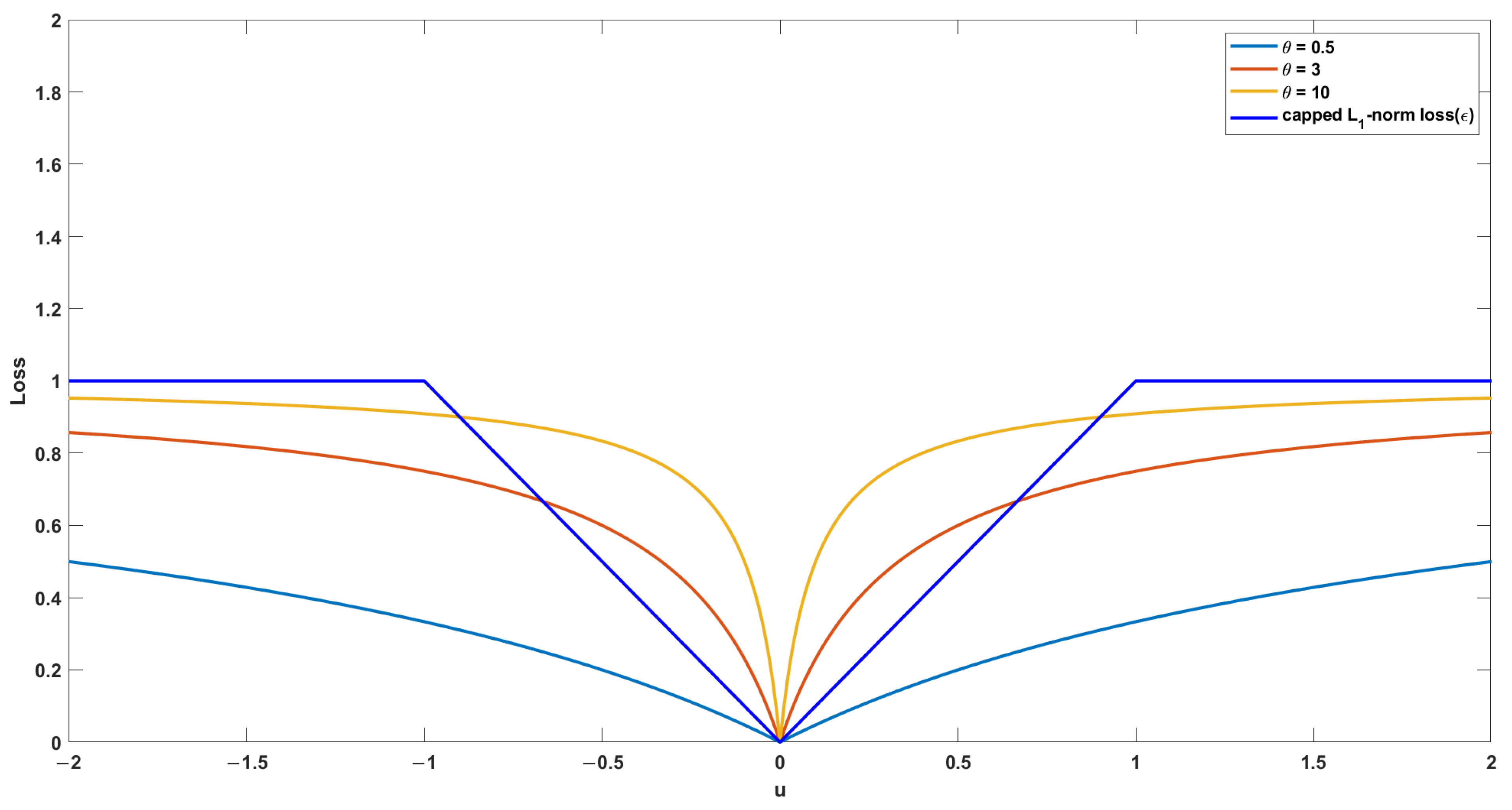
To alleviate the non-differentiable region that may be introduced by hard capped, we propose the soft-truncated SC-loss function $L_{\theta }$ as follows:

Definition 1.

Given a vector u, the $L_{\theta }$ function is defined as

$$\begin{array}{c}\hfill L_{\theta }\left(u\right)=1-{\displaystyle \frac{1}{1+\theta \left|u\right|}}\end{array}$$

(16)

where $\theta \ge 0$ is the adaptive parameter of the loss function. For example, as shown in Figure 2, the capped $L_1$-norm ($ϵ=1$) loss is non-differentiable at $u=1$, and our proposed $L_{\theta }$-loss can avoid this problem, thus making it more convenient for us when dealing with it.

The following are some properties of the $L_{\theta }\text{-}loss$:

Theorem 1.

$L_{\theta }$ is a symmetric function.

Proof of Theorem 1.

$$\begin{array}{cc}\hfill L_{\theta }(-u)& =1-{\displaystyle \frac{1}{1+\theta |-u|}}\hfill \\ \hfill & =1-{\displaystyle \frac{1}{1+\theta \left|u\right|}}=L_{\theta }\left(u\right)\hfill \end{array}$$

(17)

   □

Theorem 2.

$L_{\theta }$ is a non-negative function.

Proof of Theorem 2.

$$\begin{array}{cc}\hfill L_{\theta }\left(u\right)& =1-{\displaystyle \frac{1}{1+\theta \left|u\right|}}\hfill \\ \hfill & ={\displaystyle \frac{\theta \left|u\right|}{1+\theta \left|u\right|}}\ge 0\hfill \end{array}$$

(18)

   □

Theorem 3.

$L_{\theta }$ is a bounded function.

Proof of Theorem 3.

$$\begin{array}{cc}\hfill \underset{u\to \infty }{lim}{L}_{\theta }\left(u\right)& =1-{\displaystyle \frac{1}{1+\theta \left|u\right|}}\hfill \\ \hfill & =1\hfill \end{array}$$

(19)

   □

Remark 1.

Here, 1 is the maximum value of $L_{\theta }\left(u\right)$, which determines the last term of the loss function and is therefore robust.

3.2. Linear SCTELM

Based on (11), (12) and our proposed $L_{\theta }$-loss function, we can obtain the formula for SCTELM, expressed as follows:

SCTELM1: 

$$\underset{{\beta }_1}{min}{\displaystyle \frac{1}{2}}{\parallel U{\beta }_1\parallel }^2+C_1\sum _{i=1}^{l_2}(1-{\displaystyle \frac{1}{1+\theta |1+h\left(x_i\right){\beta }_1|}})$$

(20)

SCTELM2: 

$$\underset{{\beta }_2}{min}{\displaystyle \frac{1}{2}}{\parallel V{\beta }_2\parallel }^2+C_2\sum _{j=1}^{l_2}(1-{\displaystyle \frac{1}{1-\theta |1+h\left(x_j\right){\beta }_2|}})$$

(21)

for SCTELM1, substituting ${\beta }_1=-{(U^{T}U+{ϵ}_{1}I)}^{-1}{V}^T\alpha$ into $\parallel U{\beta }_1{\parallel }^2$ gives

$$\begin{array}{cc}\hfill \parallel U{\beta }_1{\parallel }^2& ={\left(U{\beta }_1\right)}^T\left(U{\beta }_1\right)\hfill \\ \hfill & ={[-U{(U^{T}U+{ϵ}_{1}I)}^{-1}{V}^T\alpha ]}^T[-U{(U^{T}U+{ϵ}_{1}I)}^{-1}{V}^T\alpha ]\hfill \\ \hfill & ={\alpha }^{T}V{(U^{T}U+{ϵ}_{1}I)}^{-1}{U}^{T}U{(U^{T}U+{ϵ}_{1}I)}^{-1}{V}^T\alpha \hfill \end{array}$$

(22)

Let $D_1={(U^{T}U+ϵI)}^{-1}{U}^{T}U{(U^{T}U+ϵI)}^{-1}$; there is

$$\begin{array}{cc}\hfill \parallel U{\beta }_1{\parallel }^2& ={\left(U{\beta }_1\right)}^T\left(U{\beta }_1\right)\hfill \\ \hfill & ={\alpha }^{T}V{D}_1{V}^T\alpha \hfill \\ \hfill & =\sum _{i=1}^{l_2}{\alpha }_{i}h\left(x_i\right)D_1\sum _{k=1}^{l_2}h{\left(x_k\right)}^T{\alpha }_k\hfill \\ \hfill & =\sum _{i=1}^{l_2}\sum _{k=1}^{l_2}{\alpha }_i{\alpha }_{k}h\left(x_i\right)D_{1}h{\left(x_k\right)}^T\hfill \end{array}$$

(23)

Substituting ${\beta }_1=-{(U^{T}U+ϵI)}^{-1}{V}^T\alpha$ into $h\left(x_i\right){\beta }_1$ gives

$$\begin{array}{cc}\hfill h\left(x_i\right){\beta }_1& =-h\left(x_i\right){(U^{T}U+ϵI)}^{-1}{V}^T\alpha \hfill \end{array}$$

(24)

Let $E_1={(U^{T}U+ϵI)}^{-1}$; there is

$$\begin{array}{cc}\hfill h\left(x_i\right){\beta }_1& =-h\left(x_i\right)E_1{V}^T\alpha \hfill \\ \hfill & =-h\left(x_i\right)E_1\sum _{k=1}^{l_2}h{\left(x_k\right)}^T{\alpha }_k\hfill \\ \hfill & =-\sum _{k=1}^{l_2}{\alpha }_{k}h\left(x_i\right)E_{1}h{\left(x_k\right)}^T\hfill \end{array}$$

(25)

Thus, (20) can be expressed as

$$\begin{array}{c}\hfill \underset{{\alpha }_i}{min}{\displaystyle \frac{1}{2}}\sum _{i=1}^{l_2}\sum _{k=1}^{l_2}{\alpha }_i{\alpha }_{k}h\left(x_i\right)D_{1}h{\left(x_k\right)}^T+C_1\sum _{i=1}^{l_2}\left(1-{\displaystyle \frac{1}{1+\theta |1-{\sum }_{k=1}^{l_2}{\alpha }_{k}h\left(x_i\right)E_{1}h{\left(x_k\right)}^T|}}\right)\end{array}$$

(26)

For a given sample $x_i$, its objective function is denoted by

$$\begin{array}{c}\hfill f_i\left(\alpha \right)={\displaystyle \frac{1}{2}}\sum _{k=1}^{l_2}{\alpha }_i{\alpha }_{k}h\left(x_i\right)D_{1}h{\left(x_k\right)}^T+C_1\left(1-{\displaystyle \frac{1}{1+\theta |1-{\sum }_{k=1}^{l_2}{\alpha }_{k}h\left(x_i\right)E_{1}h{\left(x_k\right)}^T|}}\right)\end{array}$$

(27)

If $1-{\sum }_{k=1}^{l_2}{\alpha }_{j}h\left(x_i\right)E_{1}h{\left(x_k\right)}^T\le 0$, there is

$$\begin{array}{cc}\hfill f_i\left(\alpha \right)& ={\displaystyle \frac{1}{2}}\sum _{k=1}^{l_2}{\alpha }_i{\alpha }_{k}h\left(x_i\right)D_{1}h{\left(x_k\right)}^T+C_1\left(1-{\displaystyle \frac{1}{1+\theta ({\sum }_{j=1}^{l_2}{\alpha }_{k}h\left(x_i\right)E_{1}h{\left(x_k\right)}^T-1)}}\right)\hfill \\ \hfill & ={\displaystyle \frac{1}{2}}\sum _{k=1}^{l_2}{\alpha }_i{\alpha }_{k}h\left(x_i\right)D_{1}h{\left(x_k\right)}^T+{\displaystyle \frac{C_1\theta ({\sum }_{k=1}^{l_2}{\alpha }_{k}h\left(x_i\right)E_{1}h{\left(x_k\right)}^T-1)}{1+\theta ({\sum }_{k=1}^{l_2}{\alpha }_{k}h\left(x_i\right)E_{1}h{\left(x_k\right)}^T-1)}}\hfill \end{array}$$

(28)

Let ${\xi }_i\left(\alpha \right)=1-{\sum }_{k=1}^{l_2}{\alpha }_{k}h\left(x_i\right)E_{1}h{\left(x_k\right)}^T$, there is

$$\begin{array}{c}\hfill f_i\left(\alpha \right)={\displaystyle \frac{1}{2}}\sum _{k=1}^{l_2}{\alpha }_i{\alpha }_{k}h\left(x_i\right)D_{1}h{\left(x_k\right)}^T-{\displaystyle \frac{C_1\theta {\xi }_i\left(\alpha \right)}{1-\theta {\xi }_i\left(\alpha \right)}}\end{array}$$

(29)

and the gradient of $f_i\left(\alpha \right)$ with respect to $\alpha$ can be represented by

$$\begin{array}{c}\hfill \nabla f_i\left(\alpha \right)={\displaystyle \frac{\partial f_i\left(\alpha \right)}{\partial \alpha }}={\displaystyle \frac{V{D}_1{V}^T\alpha }{l_2}}+{\displaystyle \frac{C_1\theta V{E}_{1}h{\left(x_i\right)}^T}{{(1-\theta {\xi }_i\left(\alpha \right))}^2}}\end{array}$$

(30)

If $1-{\sum }_{k=1}^{l_2}{\alpha }_{k}h\left(x_i\right)E_{1}h{\left(x_k\right)}^T>0$, we then have

$$\begin{array}{cc}\hfill f_i\left(\alpha \right)& ={\displaystyle \frac{1}{2}}\sum _{k=1}^{l_2}{\alpha }_i{\alpha }_{k}h\left(x_i\right)D_{1}h{\left(x_k\right)}^T+C_1\left(1-{\displaystyle \frac{1}{1+\theta (1-{\sum }_{k=1}^{l_2}{\alpha }_{k}h\left(x_i\right)E_{1}h{\left(x_k\right)}^T)}}\right)\hfill \\ \hfill & ={\displaystyle \frac{1}{2}}\sum _{k=1}^{l_2}{\alpha }_i{\alpha }_{k}h\left(x_i\right)D_{1}h{\left(x_k\right)}^T+{\displaystyle \frac{C_1\theta (1-{\sum }_{k=1}^{l_2}{\alpha }_{k}h\left(x_i\right)E_{1}h{\left(x_k\right)}^T)}{1+\theta (1-{\sum }_{k=1}^{l_2}{\alpha }_{k}h\left(x_i\right)E_{1}h{\left(x_k\right)}^T)}}\hfill \\ & ={\displaystyle \frac{1}{2}}\sum _{k=1}^{l_2}{\alpha }_i{\alpha }_{k}h\left(x_i\right)D_{1}h{\left(x_k\right)}^T+{\displaystyle \frac{C_1\theta {\xi }_i\left(\alpha \right)}{1+\theta {\xi }_i\left(\alpha \right)}}\hfill \end{array}$$

(31)

and the gradient of $f_i\left(\alpha \right)$ with respect to $\alpha$ can be represented by

$$\begin{array}{c}\hfill \nabla f_i\left(\alpha \right)={\displaystyle \frac{\partial f_i\left(\alpha \right)}{\partial \alpha }}={\displaystyle \frac{V{D}_1{V}^T\alpha }{l_2}}-{\displaystyle \frac{C_1\theta V{E}_{1}h{\left(x_i\right)}^T}{{(1+\theta {\xi }_i\left(\alpha \right))}^2}}\end{array}$$

(32)

Combining (30) and (32), the gradient of $f_i\left(\alpha \right)$ with respect to $\alpha$ can be represented by

$$\begin{array}{c}\hfill \nabla f_i\left(\alpha \right)={\displaystyle \frac{V{D}_1{V}^T\alpha }{l_2}}-{\displaystyle \frac{C_1\theta V{E}_{1}h{\left(x_i\right)}^T}{{(1+sgn\left({\xi }_i\left(\alpha \right)\right)\theta {\xi }_i\left(\alpha \right))}^2}}sgn\left({\xi }_i\left(\alpha \right)\right)\end{array}$$

(33)

Then, the average gradient over l samples can be computed as

$$\begin{array}{cc}\hfill \nabla R_{l_2}& ={\displaystyle \frac{1}{l_2}}\sum _{i=1}^{l_2}\nabla f_i\left(\alpha \right)\hfill \\ \hfill & ={\displaystyle \frac{V{D}_1{V}^T\alpha }{l_2}}-{\displaystyle \frac{C_1\theta V{E}_1}{l_2}}\sum _{i=1}^{l_2}{\displaystyle \frac{h{\left(x_i\right)}^T}{{(1+sgn\left({\xi }_i\left(\alpha \right)\right)\theta {\xi }_i\left(\alpha \right))}^2}}sgn\left({\xi }_i\left(\alpha \right)\right)\hfill \end{array}$$

(34)

The same can be said for the following:

$$\begin{array}{cc}\hfill \nabla f_j\left(\gamma \right)& ={\displaystyle \frac{U{D}_2{U}^T\gamma }{l_1}}-{\displaystyle \frac{C_2\theta U{E}_{2}h{\left(x_j\right)}^T}{{(1+sgn\left({\eta }_j\left(\gamma \right)\right)\theta {\eta }_j\left(\gamma \right))}^2}}sgn\left({\eta }_j\left(\gamma \right)\right)\hfill \end{array}$$

(35)

$$\begin{array}{cc}\hfill \nabla R_{l_1}& ={\displaystyle \frac{U{D}_2{U}^T\gamma }{l_1}}-{\displaystyle \frac{C_2\theta U{E}_2}{l_1}}\sum _{j=1}^{l_1}{\displaystyle \frac{h{\left(x_j\right)}^T}{{(1+sgn\left({\eta }_j\left(\gamma \right)\right)\theta {\eta }_j\left(\gamma \right))}^2}}sgn\left({\eta }_j\left(\gamma \right)\right)\hfill \end{array}$$

(36)

where $D_2={(V^{T}V+{ϵ}_{2}I)}^{-1}{V}^{T}V{(V^{T}V+{ϵ}_{2}I)}^{-1},{\eta }_j\left(\gamma \right)=1-{\sum }_{m=1}^{l_1}{\gamma }_{m}h\left(x_j\right)D_{2}h{\left(x_m\right)}^T$, $E_2={(V^{T}V+{ϵ}_{2}I)}^{-1}$. From the above equation, we can obtain ${\alpha }^{\ast },{\gamma }^{\ast }$; when we obtain a new sample vector x, we can make predictions according to the following decision function:

$$\begin{array}{c}\hfill f\left(x\right)=argmin\left\{\right|-h\left(x\right){(U^{T}U+{ϵ}_{2}I)}^{-1}{V}^T{\alpha }^{\ast }|,|h\left(x\right){(V^{T}V+{ϵ}_{2}I)}^{-1}{U}^T{\gamma }^{\ast }\left|\right\}\end{array}$$

(37)

3.3. Nonlinear SCTELM

Sometimes, we will encounter datasets that are not linearly separable. In such a case, we can extend SCTELM to the nonlinear case by considering the surfaces generated by the following two kernels:

$$\begin{array}{c}\hfill K_{ELM}(x^T,G^T){\beta }_1=0,\\ \hfill K_{ELM}(x^T,G^T){\beta }_2=0,\end{array}$$

(38)

where $G=(A;B)$, and $K_{ELM}$ is the kernel function of ELM, which can be expressed as $K_{ELM}=h\left(x_i\right)h\left(x_j\right)$. From this, the original problem of TELM can be expressed as follows:

$$\begin{array}{cc}\hfill & \underset{{\beta }_1,\xi }{min}{\displaystyle \frac{1}{2}}{\parallel K_{ELM}(A^T,G^T){\beta }_1\parallel }_2^2+C_1{e}_2^T\xi \hfill \\ \hfill & s.t-K_{ELM}(B^T,G^T){\beta }_1+\xi \ge e_2,\xi \ge 0.\hfill \end{array}$$

(39)

$$\begin{array}{cc}\hfill & \underset{{\beta }_2,\eta }{min}{\displaystyle \frac{1}{2}}{\parallel K_{ELM}(B^T,G^T){\beta }_2\parallel }_2^2+C_2{e}_1^T\eta \hfill \\ \hfill & s.t{K}_{ELM}(A^T,G^T){\beta }_2+\eta \ge e_1,\eta \ge 0.\hfill \end{array}$$

(40)

From the KKT condition, we can obtain ${\beta }_1=-{(R^{T}R+ϵI)}^{-1}{S}^T\alpha$ and  ${\beta }_2={(S^{T}S+ϵI)}^{-1}{R}^T\gamma$, where $R=K_{ELM}(A^T,G^T)$ and $S=K_{ELM}(B^T,G^T)$, and $\alpha and\gamma$ are Lagrange multipliers. The original problem for SCTELM then becomes the following:

SCTELM1: 

$$\underset{{\beta }_1}{min}{\displaystyle \frac{1}{2}}{\parallel K_{ELM}(A^T,G^T){\beta }_1\parallel }^2+C_1\sum _{i=1}^{l_2}(1-{\displaystyle \frac{1}{1+\theta |1+h\left(x_i\right){\beta }_1|}})$$

(41)

SCTELM2: 

$$\underset{{\beta }_2}{min}{\displaystyle \frac{1}{2}}{\parallel K_{ELM}(B^T,G^T){\beta }_2\parallel }^2+C_2\sum _{j=1}^{l_2}(1-{\displaystyle \frac{1}{1-\theta |1+h\left(x_j\right){\beta }_2|}})$$

(42)

Following the way linear SCTELM is computed, we can obtain the following, according to SCTELM1:

$$\begin{array}{c}\hfill \nabla f_i\left(\alpha \right)={\displaystyle \frac{V{D}_3{S}^T\alpha }{l_2}}-{\displaystyle \frac{C_1\theta S{E}_{3}h{\left(x_i\right)}^T}{{(1+sgn\left({\xi }_i\left(\alpha \right)\right)\theta {\xi }_i\left(\alpha \right))}^2}}sgn\left({\xi }_i\left(\alpha \right)\right)\end{array}$$

(43)

$$\begin{array}{c}\hfill \nabla R_{l_2}=={\displaystyle \frac{S{D}_3{S}^T\alpha }{l_2}}-{\displaystyle \frac{C_1\theta S{E}_3}{l_2}}\sum _{i=1}^{l_2}{\displaystyle \frac{h{\left(x_i\right)}^T}{{(1+sgn\left({\xi }_i\left(\alpha \right)\right)\theta {\xi }_i\left(\alpha \right))}^2}}sgn\left({\xi }_i\left(\alpha \right)\right)\end{array}$$

(44)

and according to SCTELM2:

$$\begin{array}{cc}\hfill \nabla f_j\left(\gamma \right)& ={\displaystyle \frac{R{D}_4{R}^T\gamma }{l_1}}-{\displaystyle \frac{C_2\theta R{E}_{4}h{\left(x_j\right)}^T}{{(1+sgn\left({\eta }_j\left(\gamma \right)\right)\theta {\eta }_j\left(\gamma \right))}^2}}sgn\left({\eta }_j\left(\gamma \right)\right)\hfill \end{array}$$

(45)

$$\begin{array}{cc}\hfill \nabla R_{l_1}& ={\displaystyle \frac{R{D}_4{R}^T\gamma }{l_1}}-{\displaystyle \frac{C_2\theta R{E}_4}{l_1}}\sum _{j=1}^{l_1}{\displaystyle \frac{h{\left(x_j\right)}^T}{{(1+sgn\left({\eta }_j\left(\gamma \right)\right)\theta {\eta }_j\left(\gamma \right))}^2}}sgn\left({\eta }_j\left(\gamma \right)\right)\hfill \end{array}$$

(46)

where $D_3={(R^{T}R+{ϵ}_{2}I)}^{-1}{R}^{T}R=R{(R^{T}R+{ϵ}_{2}I)}^{-1},E_3={(R^{T}R+{ϵ}_{2}I)}^{-1},{\zeta }_i\left(\alpha \right)=1-{\sum }_{k=1}^{l_2}{\alpha }_{k}h\left(x_i\right)E_{3}h{\left(x_k\right)}^T,D_4={(R^{T}R+{ϵ}_{2}I)}^{-1}{R}^{T}R=R{(R^{T}R+{ϵ}_{2}I)}^{-1},E_4={(R^{T}R+{ϵ}_{2}I)}^{-1},{\rho }_j\left(\gamma \right)=1-{\sum }_{m=1}^{l_1}{\gamma }_{m}h\left(x_j\right)E_{4}h{\left(x_m\right)}^T.$ In the same way, from the above equation, we can obtain ${\alpha }^{\ast },{\gamma }^{\ast }$. When we obtain a new sample vector x, we can make predictions according to the following decision function:

$$\begin{array}{c}\hfill f\left(x\right)=argmin\left\{\right|-h\left(x\right){(R^{T}R+{ϵ}_{2}I)}^{-1}{S}^T{\alpha }^{\ast }|,|h\left(x\right){(S^{T}S+{ϵ}_{2}I)}^{-1}{R}^T{\gamma }^{\ast }\left|\right\}\end{array}$$

(47)

3.4. Convergence Analysis

Consider a fixed-stage n in Algorithm 1. Let ${\omega }^{\ast }=arg\underset{\alpha }{min}f\left(\alpha \right)$. Assume that m is sufficiently large and, therefore,

$$\begin{array}{c}\hfill \eta ={\displaystyle \frac{1}{P\tau (1-2K\tau )T}}+{\displaystyle \frac{2K\tau }{1-2K\tau }}<1\end{array}$$

(48)

Then, we can determine that the expectation on SVRG has geometric convergence, as follows:

$$\begin{array}{c}\hfill \mathbb{E}\left[f\left({\tilde{\omega }}_n\right)\right]\le \mathbb{E}\left[f\left({\omega }^{\ast }\right)\right]+\eta \mathbb{E}[f\left({\tilde{\omega }}_{n-1}\right)-f\left({\omega }^{\ast }\right)]\end{array}$$

(49)

where $K>P>0and\tau <{\displaystyle \frac{1}{K}}$. For a detailed proof, see the work of Johnson and Zhang (2013) [25].

Algorithm 1 SVRG for SCTELM

Input: Training data $A\in {\mathbb{R}}^{l_1\times n}$ and $B\in {\mathbb{R}}^{l_2\times n}$; Parameters $\theta ,C_i,(i=1,2)$, ${\epsilon }_i,(i=1,2)$, update frequency m and learning rate $\tau$. Output: ${\tilde{\omega }}_n$.  Initialize ${\tilde{\omega }}_0$; FOR n = 1, 2, 3, ⋯, N;      $\tilde{\omega }={\tilde{\omega }}_{n-1}$;      Calculate $\nabla R_{l_1}and\nabla R_{l_2}$ according to (34) and (36) for SCTELM and (44) and (46) for Nonlinear SCTELM;      FOR t = 1, 2, 3, ⋯, T;      Randomly pick $i_t\in \{1,2,3,\cdots ,l\}$;      Update weight ${\omega }_t={\omega }_{t-1}-\tau (\nabla f_{i_t}\left({\omega }_{t-1}\right)-\nabla f_{i_t}\left(\tilde{\omega }\right)+\nabla R_l\left(\tilde{\omega }\right))$ according to (33) and (35) for SCTELM and (43) and (45) for Nonlinear SCTELM;      END      ${\tilde{\omega }}_n={\omega }_m$;  END

3.5. Computational Complexity Analysis

In this section, we briefly analyze the complexity of the proposed algorithm. Here, we only compute the linear SCTELM, and similarly, the nonlinear SCTELM, which is well known to be determined by the computational cost and the number of iterations. First, we analyze the former; the computational complexity of $D_1$ and $D_2$ in (33) and (35) is $O(l\times L^2+L^3)$, while the computational complexity of $E_1$ and $E_2$ is $O(l\times L^2+L^3)$, so the overall complexity of (33) and (35) is $O(l\times L^2+L^3)$. Similarly, the complexity of (34) and (36) is $O\left(L^3\right)$. In Algorithm 1, the outer loop is executed N times and the inner loop is executed T times, so the total computational cost of the algorithm is $O\left(NT(l\times L^2+L^3)\right)$. While L is the number of neurons, there is usually $L\ll l$, so the complexity of Algorithm 1 is $O(NTl\times L^2)$. It can be seen that the complexity of the SCTELM algorithm is mainly affected by the number of samples, and the convergence speed of the SVRG algorithm is faster than that of other algorithms, so the convergence speed of the SCTELM algorithm is faster than that of other algorithms.

SVRG reduces the variance of the stochastic gradient by introducing an estimate of the global gradient, thus improving the convergence speed. This means that in each iteration, SVRG can use fewer samples (mini-batch) to achieve the same accuracy as traditional SGD. This variance reduction property makes the algorithm more efficient when dealing with large-scale data, thus improving the scalability. Each iteration of SVRG needs to calculate the global gradient, which increases a certain computational overhead compared with only calculating the gradient of local samples. However, due to its faster convergence speed, the same performance can usually be achieved in a smaller number of iterations, thus reducing the overall computation time on large-scale datasets.

4. Numerical Experiments

In this section, to evaluate the robustness of SCTELM, we systematically compare it with other advanced algorithms in multiple datasets, including ELM [2], LELM [26], CTSVM [18],CHELM [27], TELM [24], and FRTELM [28]. For ease of observation, the bold font in the table below indicates the optimum. After dataset testing, we also performed classification visualization to further embody the performance of our proposed model. All experiments were performed using the Windows operating system with a 12th generation Intel (R) core (TM), i7-6700HQ @ 2.10 GHz, and 8.00 GB RAM, and the environment was implemented on a PC running a 64-bit XP operating system. All codes were run by MATLAB R2021b.

4.1. Experimental Setup

We can evaluate the performance of an algorithm based on different metrics, but here, we will use accuracy (ACC), which measures the proportion of instances that the model correctly predicted. ACC is defined as follows:

$$\begin{array}{c}\hfill ACC={\displaystyle \frac{TP+TN}{TP+FP+TN+FN}}\end{array}$$

(50)

where TP and TN represent true positive and true negative, respectively, which represent the correct prediction of positive and negative samples; FP and FN represent false positive and false negative, respectively, which represent the incorrect prediction of positive and negative samples. Among them, a higher ACC value represents a more accurate classification and a better model performance.

In our experiment design, the training and testing samples were randomly selected from the dataset, and we added outliers of 0%, 10%, 20%, and 30% to the training set, respectively, and used these contaminated training samples to verify the robustness of the model. In this experiment, due to the large number of parameters, we used the random search method to find the best parameters. The parameters selected for the proposed model are as follows: parameter $C_i$ is selected from the set $\left\{{10}^i\right|i=-5,-4,-3,-2,-1,0,1,2,3,4,5\}$, and parameter ${\epsilon }_i$ is selected from the set $\left\{{10}^i\right|i=-5,-4,-3,-2,-1,0,1,2,3,4,5\}$.

4.2. Description of the Datasets

To verify the performance of our proposed SCTELM, we will numerically simulate it using various datasets, including eight benchmark datasets from UCI and two artificial datasets.

Among them, the UCI dataset includes the following: Australian (Australian Credit Approval), Ionosphere, German, Pima, Vote (Congressional Voting Records), WDBC (Breast Cancer Wisconsin), Spect (SPECTF Heart) and QSAR (QSAR biodegradation). We will use these UCI datasets to compare the performance of our proposed algorithm with other algorithms. See

Table 1. Characteristics of the UCI datasets.

Datasets	Samples	Attributes	Positive Samples	Negative Samples
Australian	690	14	307	383
VOTE	432	16	167	265
WDBC	569	30	357	212
Spect	267	44	212	55
QSAR	1055	41	699	356
Ionosphere	351	34	225	126
German	1000	24	700	300
Pima	768	8	500	268

for relevant information on these datasets.

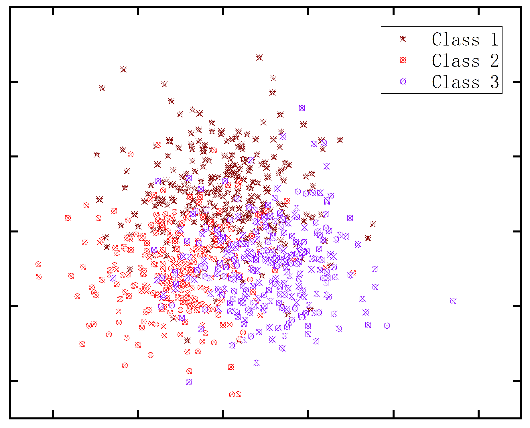
In terms of artificial datasets, we generated a two moons dataset containing two categories, 1000 positive and 1000 negative, and a dataset containing three categories. See Figure 3 for the detailed dataset, where the positive and negative classes are represented by green and orange spheres. And the three-classification dataset contains 900 samples, and each class has 300 samples. See Figure 4 for details.

We performed a 10-fold cross-validation on the selected datasets, which means that we randomly split one of the datasets into ten parts, nine of which were used as the training set and the remaining one as the test set. This process was repeated ten times, and the average of the ten results was taken as the final performance metric to reduce the risk of overfitting and underfitting. At the same time, to obtain more objective experimental results, we normalized all the datasets to make the data in the interval [0, 1]. Considering that we want to verify the robust performance of the model, we will successively increase the noise ratio for each dataset. If the accuracy of classification does not change much with the increase in noise, it indicates that the algorithm has good robust performance.

4.3. Experimental Results on Artificial Datasets

In order to verify the advantages of the proposed model over other original models, only ELM and TELM will be compared in this section. Observing

Table 2. Performance on artificial datasets.

	ELM	TELM	SCTELM
Noise Ratio	ACC (%)	ACC (%)	ACC (%)
0	92.53	93.82	95.91
0.1	90.16	90.50	94.64
0.2	85.31	86.73	91.36
0.3	76.64	77.55	83.45

, it can be found that when the noise ratio is zero, the accuracy of SCTELM is higher than that of TELM and ELM, which indicates that SCTELM performs better than TELM and ELM. When the noise ratio is 0.1, the accuracy of the model is all reduced, which indicates that noise does affect the performance of the model. When the noise ratio is 0.2, the accuracy of all the models slightly decreases, but the accuracy of SCTELM is higher than that of TELM and ELM. When the noise ratio is 0.3, the accuracy of SCTELM decreases slightly, while the accuracy of ELM and TELM decreases more, which clearly illustrates the robustness of SCTELM.

To make a more intuitive comparison, the line chart of the proposed model and other models under different noises is drawn in Figure 5. It can be seen from Figure 5 that the corresponding line of SCTELM is always higher than that of the other models, which indicates that the performance of SCTELM is better than that of the other two models. When the noise gradually increases, the accuracy of all the models shows a decreasing trend, which indicates that noise does have a large impact on the performance of the model. It can be seen from the figure that when the noise rises from 0.2 to 0.3, the accuracy decline rate of ELM and TELM is faster than that of SCTELM, which also precisely demonstrates the superior robustness of the proposed model.

To extend SCRELM to the multi-class case, we adopted an artificial dataset with three classes. Generally speaking, either one-to-one or one-to-many strategy is used when using models such as ELM or TELM for multi-classification. Here, we use the more commonly used one-to-one strategy for classification. The strategy decomposes a three-class classification problem into three two-class classification problems, each of which is responsible for solving a pair of classes. The final classification results are determined by voting technology. The final results of classification are given in

Table 3. Experimental results of multi-classification artificial datasets.

	ELM	TELM	SCTELM
	ACC (%)	ACC (%)	ACC (%)
Class 1	63.74	77.83	85.17
Class 2	79.31	71.17	84.33
Class 3	72.83	73.00	83.17
Final result	71.85	74.00	84.22

. As expected, SCTELM shows its amazing ability and outperforms ELM and TELM in the final classification accuracy.

4.4. Experimental Results on UCI Datasets

In this section, to validate the classification performance algorithms, we ran them on eight datasets. We preliminarily verified the robustness of the SCTELM algorithm on the previous artificial datasets. Here, to further verify its robustness, we will add 20% and 30% Gaussian noise to all datasets. See

Table 4. Experimental results on UCI datasets without noise.

	ELM	TELM	LELM	CTSVM	CHELM	FRTELM	SCTELM
Datasets	ACC (%)	ACC (%)	ACC (%)	ACC (%)	ACC (%)	ACC (%)	ACC (%)
	Times (s)	Times (s)	Times (s)	Times (s)	Times (s)	Times (s)	Times (s)
Australian	84.37	85.71	84.57	85.64	84.93	85.73	86.32
	1.431	1.983	0.793	0.324	3.368	1.173	0.601
WDBC	95.31	97.32	96.54	97.31	96.86	97.67	98.21
	1.3546	0.924	0.734	0.847	2.736	0.514	0.525
QSAR	83.94	85.63	85.31	85.19	86.17	86.37	86.51
	1.374	0.561	1.351	1.169	3.483	0.437	1.659
German	76.59	77.80	78.62	76.57	76.88	77.63	78.55
	1.709	1.093	2.018	1.687	5.021	0.729	1.486
Vote	95.19	95.52	96.35	95.51	96.47	97.03	97.62
	1.244	0.821	0.465	0.656	4.076	0.519	0.339
Spect	81.37	82.71	82.68	82.25	81.96	82.94	83.62
	0.770	0.831	0.769	1.132	1.982	0.492	0.250
Ionosphere	86.33	88.00	90.67	88.60	87.65	91.08	91.37
	0.589	0.361	0.363	0.399	2.561	0.229	0.264
Pima	76.12	76.31	75.97	76.92	76.78	77.13	77.83
	1.854	1.008	1.105	1.317	3.561	1.347	0.539
Avg. ACC	84.90	86.13	86.34	86.00	85.96	87.07	87.50
Avg. rank	6.75	4.00	4.45	4.88	4.63	2.13	1.13

,

Table 5. Experimental results on UCI datasets with 20% Gaussian noise.

	ELM	TELM	LELM	CTSVM	CHELM	FRTELM	SCTELM
Datasets	ACC (%)	ACC (%)	ACC (%)	ACC (%)	ACC (%)	ACC (%)	ACC (%)
	Times (s)	Times (s)	Times (s)	Times (s)	Times (s)	Times (s)	Times (s)
Australian	75.74	76.34	75.97	77.49	78.53	79.81	81.88
	1.371	0.983	0.893	0.781	6.368	1.469	0.330
WDBC	85.49	83.72	84.14	86.72	86.95	89.74	92.86
	1.478	1.124	1.715	1.195	8.969	1.649	0.791
QSAR	64.73	66.81	65.29	65.73	65.29	69.52	73.29
	2.314	4.539	2.059	2.994	10.237	2.784	1.728
German	68.93	67.38	68.19	68.71	69.71	71.37	72.30
	2.539	2.348	1.818	1.434	4.320	1.647	0.965
Vote	91.72	93.57	91.29	91.03	94.27	94.54	95.86
	0.909	0.495	0.965	0.938	3.867	1.652	0.439
Spect	70.09	72.49	70.18	80.63	80.34	80.63	81.77
	0.759	1.095	0.819	1.151	5.184	1.525	0.375
Ionosphere	78.37	81.54	79.74	79.35	79.52	83.39	83.82
	0.889	2.539	0.751	0.804	4.264	1.257	0.350
Pima	65.71	65.40	66.74	71.74	72.78	72.37	73.34
	1.804	0.943	0.905	1.032	2.553	1.561	0.711
Avg. ACC	75.10	75.91	75.19	77.68	78.42	80.25	81.89
Avg. rank	6.00	5.13	5.50	4.50	3.63	2.00	1.00

and

Table 6. Experimental results on UCI datasets with 30% Gaussian noise.

	ELM	TELM	LELM	CTSVM	CHELM	FRTELM	SCTELM
Datasets	ACC (%)	ACC (%)	ACC (%)	ACC (%)	ACC (%)	ACC (%)	ACC (%)
	Times (s)	Times (s)	Times (s)	Times (s)	Times (s)	Times (s)	Times (s)
Australian	64.81	63.62	63.94	67.32	68.01	74.84	75.74
	1.746	1.493	1.513	1.641	6.468	1.426	0.494
WDBC	62.53	63.03	63.53	74.83	74.57	79.41	80.36
	1.71	1.548	1.585	1.835	8.361	1.457	1.451
QSAR	62.79	63.72	62.53	66.36	66.76	69.36	70.04
	2.856	4.792	3.283	2.186	10.593	3.429	1.994
German	67.29	67.98	69.52	62.93	68.71	69.37	69.80
	3.094	2.429	2.043	3.184	4.302	1.827	1.029
Vote	91.61	90.78	92.33	91.97	93.67	93.91	94.10
	0.749	0.765	0.649	1.098	3.625	1.372	0.372
Spect	62.92	65.97	64.42	78.34	78.57	78.87	79.54
	0.963	0.961	0.913	1.241	4.215	1.500	0.321
Ionosphere	72.72	67.04	72.79	75.05	74.01	75.19	75.59
	0.859	0.979	0.811	0.972	3.683	1.017	0.350
Pima	63.91	64.22	62.94	67.88	68.58	70.63	72.11
	1.673	1.263	0.734	0.371	2.102	1.527	0.729
Avg. ACC	68.57	68.30	69.00	73.09	74.11	76.47	77.16
Avg. rank	6.13	5.88	5.38	4.25	3.38	2.00	1.00

for details. However, the choice to set 20% or 30% noise in the SCTELM algorithm experiment can, on the one hand, simulate a data bias that may exist in the real environment to evaluate the performance of the model in the face of noisy data. A clearer understanding of the anti-noise performance of the SCTELM algorithm can be obtained by comparing the experimental results under different noise levels. For example, if the model performs well under 30% noise, it is robust to noise. On the other hand, the increase in noise level will increase the complexity and randomness of the data, making the distribution difference between the training data and the test data larger. Whether the SCTELM model can maintain good generalization performance when the noise is high reflects its ability to adapt to unseen data. All in all, this setting is useful for assessing how well the model generalizes on test sets or real-world application data.

4.4.1. Experimental Results on UCI Datasets Without Outliers

From Table 4, we can clearly find that the classification performance of our proposed SCTELM is better than the other five algorithms on all datasets. In addition, we also find that TELM and CTSVM are faster than the other algorithms on most datasets, this is because they solve one large QPPs instead of two small QPPs. Our proposed algorithm also inherits this advantage. It can be clearly seen in Table 4 that the learning efficiency of SCTELM is ahead of other algorithms in most datasets.

4.4.2. Experimental Results on UCI Datasets with Outliers

We verified the superiority of SCTELM in the previous experiments. To further verify the robustness of SCTELM, we added a certain proportion of outliers in each dataset and conduct new experiments. In this experiment, we chose to add 20% and 30% Gaussian noise, respectively, to test the robustness of the model. Table 5 and Table 6 present the experimental results of the six models with 20% and 30% noise introduced, respectively. From Table 5 and Table 6, we can intuitively find that the accuracy of each model decreases after the introduction of noise, which indicates that noise pollution indeed has a great impact on model classification. At the same time, we can also find that the accuracy of the SCTELM model still maintains its superiority, and it can be concluded that the robustness of our proposed SCTELM model is significantly better than the robustness of other models.

In order to improve our intuition, we drew Figure 6, Figure 7, Figure 8 and Figure 9 according to the noise ratio and accuracy. From the figure, we can clearly see that the accuracy decreases when the noise increases, and we can also intuitively see that the “slope” of SCTELM is small. It further shows that SCTELM has strong robustness.

4.5. Statistical Analysis

In this section, to analyze the significant differences in the six presented algorithms on these eight UCI datasets, we conducted the Friedman test [29], which is considered as a non-parametric test with low data distribution requirements, strong processing power, and easy interpretation of the results. In this test, the null hypothesis $H_0$ is as follows: there is no significant difference between the six algorithms; and if the null hypothesis is rejected, then the Nemeny test will be performed [29]. The average ranking and average accuracy of these six algorithms on the eight datasets are shown in Table 4, Table 5 and Table 6.

First, we can make a statistical comparison according to the noise-free case, and according to the Friedman statistic formula, it can be obtained as follows:

$$\begin{array}{c}\hfill {\chi }_F^2={\displaystyle \frac{12N}{k(k+1)}}[\sum _j{R}_j^2-{\displaystyle \frac{k{(k+1)}^2}{4}}]=35.57\end{array}$$

where N is the number of datasets, k is the number of algorithms, and $R_j$ is the average ranking of the jth algorithm over all datasets. In this paper, k = 7 and N = 8.

Second, we can obtain the ${\chi }_F^2$-distribution with $(k-1)$ degrees of freedom, as follows:

$$\begin{array}{c}\hfill F_F={\displaystyle \frac{(N-1){\chi }_F^2}{N(k-1)-{\chi }_F^2}}=20.03\end{array}$$

Similarly, we can obtain that the ${\chi }_F^2$ values of noise 0.2 and 0.3 are 32.41 and 40.07, respectively, and the $F_F$ values are 9.12 and 20.48, respectively. For $\alpha =0.05$, we can obtain $F_{\alpha }=(6,42)=2.32$. Clearly, all $F_F$ has $F_F>F_{\alpha }$. Therefore, it can be said that there are significant differences between the six algorithms.

In the following, to further compare the six algorithms, the Nemenyi post hoc test will be performed. Referring to the table, we obtain $q_{\alpha =0.05}=2.85$, which gives us the critical difference (CD):

$$\begin{array}{c}\hfill CD=q_{\alpha =0.05}\sqrt{{\displaystyle \frac{k(k+1)}{6N}}}=2.85\times \sqrt{{\displaystyle \frac{7\times 8}{6\times 8}}}=3.078\end{array}$$

If the difference between the rankings of the two algorithms calculated is larger than the critical value, it represents a significant difference between the two algorithms. From Table 4, we can obtain the difference between SCTELM and the other five algorithms when there is no noise, and the calculation results are as follows:

$$\begin{array}{c}\hfill D(ELM-SCTELM)=6.75-1.13=5.62>3.078\\ \hfill D(TELM-SCTELM)=4-1.13=2.87<3.078\\ \hfill D(LELM-SCTELM)=4.5-1.13=3.37>3.078\\ \hfill D(CTSVM-SCTELM)=4.88-1.13=3.75>3.078\\ \hfill D(CHELM-SCTELM)=4.63-1.13=3.5>3.078\\ \hfill D(FRTELM-SCTELM)=2.13-1.13=1<3.078\end{array}$$

The notation D (A-B) represents the difference in average rankings between the two algorithms. We can conclude that SCTELM significantly outperforms ELM, LELM, CTSVM and CHELM on the noise-free dataset, while showing no significant difference compared to TELM and FRTELM. According to Table 4 and Table 5, it is clear that in datasets with 20% and 30% Gaussian noise, SCTELM shows a significant difference compared to ELM, TELM and LELM, but there is little difference compared to CTSVM and CHELM. To make the conclusions clear, the post hoc detection is visualized below in Figure 10.

In Figure 10, the abscissa represents the average ranking of each algorithm, and the ordinate represents the algorithms to be compared. If two algorithms overlap with respect to the abscissa, then there is no significant difference between them. From Figure 10, we can easily draw this conclusion.

4.6. Parameter Analysis

To make it more convenient for other researchers to use SCTELM, the performance of SCTELM under different parameters will be further studied from the perspective of parameters, so we chose four representative datasets Australian, German, Spect and Ionosphere). Starting from the parameters C1, C2 and $\theta$, the sensitivity of the proposed algorithm to these parameters is analyzed. At the same time, the other parameters are fixed for experiments. The experimental results are shown in Figure 11 and Figure 12.

For the parameters C1 and C2, we observe that on these datasets, the ACC values show large fluctuations as the parameters change, and the fluctuations are particularly significant on some datasets. For example, on the German dataset, when C1 and C2 are changed, the fluctuation amplitude of ACC values is close to 60%, which indicates that this dataset is very sensitive to parameter changes. In contrast, the fluctuations of datasets like Australian are relatively small, about 30%. Through further analysis, it is found that the ACC value rises significantly as the parameter C1 decreases and reaches its maximum value at the value of C1 equal to ${10}^{-4}$, indicating that a smaller C1 is more beneficial to improve the classification accuracy. Therefore, parameter C1 is suitable for selecting a smaller value to optimize the algorithm performance. On the other hand, the effect of changing the parameter C2 on the results shows a linear trend. As the value of C2 increases, the ACC value also gradually rises, and the best classification effect is achieved when the value of C2 is ${10}^4$. This indicates that appropriately increasing C2 is helpful to further improve the classification performance of the algorithm.

Compared with parameters C1 and C2, parameter $\theta$ shows relatively stable characteristics in the experiment, especially on the Australian dataset; its maximum fluctuation range is less than 2%, showing extremely strong stability. However, on the Ionosphere dataset, the parameter $\theta$ fluctuates by nearly 10%, indicating that there is still some sensitivity of $\theta$ on some datasets. Further analysis of the experimental results shows that the influence of the parameter $\theta$ on the classification accuracy shows a nonlinear trend. Setting $\theta$ in $[{10}^{-3},{10}^3]$, the algorithm performs best, indicating that the $\theta$ value in this range can effectively optimize the classification performance.

4.7. Convergence Analysis Experiments

To verify the convergence of the proposed SCTELM algorithm, experiments will be carried out on the Austrasta, German, Spect and Ionosphere datasets in this section. The experiments are similar to those carried out in Section 4.4.2, while the relevant parameters are set to establish the optimal parameters. The experimental results are shown in Figure 13.

In Figure 13, it is easy to see that the convergence condition of SCTELM steadily decreases with the increase in the number of iterations, and it converges to a stable value after a finite number of iterations, so it can be seen that the proposed SCTELM algorithm can converge within a finite number of iterations.

5. Conclusions

This paper proposes a novel robust twin extreme learning machine that employs a newly designed soft capped $L_1$-norm loss function, designated as SCTELM for brevity. In contrast to the conventional hard capped methodology, the proposed soft capped approach effectively circumvents the potential non-differentiability issues associated with hard capped, whilst retaining the beneficial aspects of the hard capped technique. The objective of this approach is to mitigate the impact of outliers on the model, thereby increasing its robustness. Furthermore, the SCTELM only requires the resolution of a pair of relatively small quadratic programming problems (QPPs), which significantly reduces the complexity associated with the resolution of large QPPs in the past. Consequently, this enhances the learning efficiency of the model. The proposed model demonstrates enhanced stability and increased computational efficiency in the presence of data anomalies. The experimental results on noise-free and noisy datasets indicate that the SCTELM model exhibits heightened robustness compared to traditional methods. This is particularly evident in datasets containing outliers, where the “slope” of the SCTELM model exhibits a more gradual incline, and the learning efficiency is superior to other methods.

Our research is of considerable importance within the academic field. This paper introduces a novel loss function based on soft capped, which enables the construction of a robust twin extreme learning machine. This provides a new perspective and methodology for the field of machine learning and has the potential to encourage subsequent researchers to pursue innovative avenues in the design of loss functions and learning algorithms, thereby promoting the further advancement of both theoretical and practical developments. Furthermore, in the context of real-world data, such as the credit card approval dataset from the University of California, Irvine (UCI), users can be classified into two distinct categories: those who are approved for credit and those who are not. It is evident that SCTELM has gained significant advantages in terms of robustness to outliers in comparison to alternative algorithms. To illustrate, WDBC represents the Diagnostic Wisconsin Breast Cancer Database, and the SCTELM approach has also yielded significant benefits. It follows, therefore, that our research has significant practical implications for the fields of finance and medical treatment. The model is capable of facilitating the provision of real-time analysis and decision support to end users. The enhancement of accuracy and stability in the model enables enterprises and healthcare facilities to effectively address decision-making challenges in intricate contexts. The model may be utilized in a multitude of domains, including, although not limited to, image processing, signal processing, and natural language processing. These fields often have to contend with data noise and uncertainty, which robust models can help to overcome, thereby improving the accuracy and reliability of results. In conclusion, our study offers a significant contribution to the field of machine learning, providing a valuable perspective on robustness research and its potential for practical applications, which will inform future research and developments.

It should be noted that the algorithm is not without its limitations. At the commencement of each cycle, the SVRG algorithm is required to calculate the full gradient of the entire dataset. Although this will facilitate convergence more rapidly than the conventional SGD algorithm, the associated computational cost may be considerable in the context of large-scale datasets, potentially leading to a reduction in the rate of algorithmic execution. In future work, it would be worthwhile to consider employing periodic random sampling in place of calculating the full gradient each time, or to investigate combining the SVRG algorithm with an adaptive learning rate optimization algorithm. This would allow the learning rate to be adaptively changed in accordance with the gradient.