Analysis of the Flash Phenomenon in Rotor Targets with a Scatter Point Model

Abstract

This paper thoroughly investigates the occurrence of the flash phenomenon in rotor targets. The flash phenomenon is discernible in rotor targets across the time and frequency domains. This phenomenon is characterized by the modulation of signal amplitude through the Singer function, resulting in periodic peaks in the time domain. The appearance of these peaks in the time domain corresponds to the presence of a corresponding frequency band in the time–frequency domain. The influence of interference between scattering points on the amplitude and phase of echo is investigated by employing the echo scattering point model and the echo analytical expression as analytical foundations. A more comprehensive examination of the mechanisms that contribute to the emergence of the flash phenomenon in the time and time–frequency domains is undertaken. Furthermore, its objective is to verify the validity of the analysis performed on the mechanism of the phenomenon. Based on theoretical investigations and simulation results, it can be concluded that the flash phenomenon observed in rotor targets is due to interference between particular scattering points. Fundamentally, it can be comprehended as a phenomenon of interference. This research achievement has specific theoretical and practical value in detecting and recognizing rotor targets.

1. Introduction

Rotor targets encompass several types of aircraft equipped with rotating blade components. These targets primarily consist of helicopters and multi-rotor drones [1,2,3]. These targets have been prevalent in warfare, rescue operations, and counter-terrorism due to their exceptional agility and cost-effectiveness. Detecting those targets by radar can induce a micro-Doppler effect due to the spinning of their blades. The micro-Doppler effect pertains to the modulation phenomena observed in radar echoes due to the micro-motion or micro-dynamics of radar targets or their components, excluding the translational motion of the center of mass [4].

Currently, there are three primary approaches for modeling radar echoes produced by targets. An approach implemented in modeling is integral modeling [5,6]. In this method, the points on the lines representing the blades are integrated to generate a comprehensive reverberation model. An approach that may be implemented is point modeling based on scattering [7,8,9,10,11]. This methodology entails the representation of the target as an assemblage of multiple scattering points and generating echoes from each scattering point while considering their individual motion characteristics. Finally, all scattering point echoes are integrated to construct an all-encompassing echo model. Radar cross-sectional area modeling [12,13] is a type of modeling that generates reverberation by calculating the radar cross-sectional area (RCS) of the target. A range of modeling techniques are utilized in the discipline, with scattering point modeling being the predominant method.

The flash phenomenon is evidenced by the radar emissions generated by these targets. When the rotor blades are rotated perpendicular to the radar line of sight, a transient flash phenomenon will manifest in the resulting echoes. At this specific instant, the amplitude of the echo in the time domain will attain its maximal value, resulting in the manifestation of a flash in the time domain. Within time–frequency analysis, the frequency components associated with the flash’s occurrence in the time domain represent the micro-Doppler characteristics. Prior studies have documented the presence of the time–frequency domain flash [7,14,15]. Due to its unique attribute, the flash phenomenon can be utilized efficiently in the target recognition process [16,17,18]. Currently, the existing literature concerning this phenomenon is insufficient. A study examining the phenomenon and its correlation with the spacing of scattering points in echo was undertaken by the authors in [7].

Nevertheless, investigation is needed to explore the fundamental mechanism of this phenomenon. The investigation by [8] scrutinized the time–frequency distribution characteristics of micromotion echoes that arise from the rotation of the rotor targets. Nevertheless, the analysis should have examined the fundamental mechanism that produced the flash following the analytical expression.

This paper undertakes a comprehensive investigation into rotor targets’ flash phenomenon in response to current research deficiencies. A comprehensive inquiry is undertaken into the flash phenomenon associated with rotor targets. By applying the echo scattering point model and an analytical expression, this analysis centers on determining how interference between scattering points influences the phase and amplitude of the echo. This study aims to evaluate the processes through which flashes occur in the time and time–frequency domains. Furthermore, this study aims to investigate the potential correlation between the incidence of the echo flash phenomenon and individual scattering points. It has been observed that the target echo is impacted by the superposition of phases at individual scattering points. The mechanism analysis for the flash phenomenon is verified by integrating time–frequency analysis of the target’s micro-Doppler properties with simulation experiments. The experimental outcomes of simulations and theoretical analysis provide support for this substantiation. The glimmering phenomenon observed in rotor targets is due to interference between scattering points. The results obtained from this research undertaking have significantly contributed to understanding the attributes of rotor targets. Furthermore, the study provides theoretical and practical significance in target detection and recognition.

2. Related Research

2.1. Signal Model of Rotor Targets

The blade echo mainly depends on the scattering coefficient, number, and position of scattering points, and the number and position of scattering points can be transformed into the distribution of scattering points on the blade. Considering the value and distribution of scattering coefficients for all scattering points, they can be mainly divided into the following four types: first, the scattering coefficient value is consistent and the scattering points are evenly spaced; second, the scattering coefficient value is consistent but the scattering point spacing is non-uniform; third, the scattering points are evenly spaced but the scattering coefficient value is not constant; fourth, both the scattering coefficient value and the scattering point spacing are non-uniform. The latter three types are non-uniform scattering, which poses significant difficulties in research and is still being studied by scholars. In this paper, the first type is defined as uniform scattering, which is the main method for constructing blade echo models. To some extent, this ignores the complexity of the target and can simplify the analysis and generate blade echo models. If the micromotion target is equivalent to several strong scattering points, it is a specific special case of the scattering point model. This model is commonly used in micromotion research for micromotion targets such as ballistic missiles and space debris. 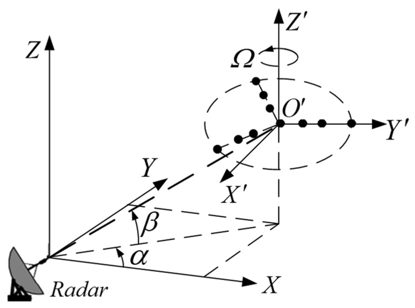Figure 1 depicts the geometric correlation between the radar and the dispersion of the target’s three rotor blades. According to [1], the baseband echo of the scattering point $P_i$ when a radar signal is transmitted at a wavelength of $\lambda$ is as follows:

$$s_{P_i}\left(t\right)=\underset{\mathrm{Amplitude} \mathrm{part}}{\underbrace{{\sigma }_{P_i}}}\underset{\mathrm{Phase} \mathrm{part}}{\underbrace{\exp \left(-j{\displaystyle \frac{4\pi R_0}{\lambda }}\right)\cdot \exp \left(-j{\displaystyle \frac{4\pi }{\lambda }}\left(x_i\cos \left({\theta }_1+2\pi f_{rot}t\right)\cos \beta \right)\right)}}.$$

(1)

Equation (1) delineates the various components of the echo: the pitch angle $\beta$, the rotor rotation frequency $f_{rot}$, the distance $x_i$ ($0\le x\le l$, $l$ is the blade length), the initial rotation angle ${\theta }_1$ between the scattering point and the rotor center, and the backscattering coefficient ${\sigma }_{P_i}$. According to Equation (1), the signal of a single scattering point can be decomposed into two distinct components: the amplitude part and the phase part.

The amplitude part is constant for a single scattering point, while the phase part is modulo 1, which does not affect the signal amplitude. The derivative of the phase of a single scattering point, which represents the instantaneous Doppler frequency of the signal emitted by that point, is illustrated in Equation (2) as follows:

$$f_{d{P}_i}\left(t\right)={\displaystyle \frac{1}{2\pi }}{\displaystyle \frac{d\varphi (t)}{dt}}={\displaystyle \frac{4\pi f_{rot}{x}_i}{\lambda }}\sin \left({\theta }_1+2\pi f_{rot}t\right)\cos \beta .$$

(2)

However, it is crucial to recognize that interference occurs among these scattering points due to a correlation between the scattering locations of the blades. The interference causes alterations to be incorporated into the echo’s amplitude and phase. In order to examine the influence of multiple scattering point superpositions on the phase component of the echo, the phase component’s instantaneous Doppler frequency of time is calculated. Additionally, Equation (3) calculates the phase component’s derivative as follows:

$$\begin{array}{ll}{f}_{d{P}_i}\left(t\right)& =-{\displaystyle \frac{1}{2\pi }}{\displaystyle \frac{d}{dt}}\exp \left(-j{\displaystyle \frac{4\pi R_0}{\lambda }}\right)\cdot \exp \left(-j{\displaystyle \frac{4\pi }{\lambda }}\left(x_i\cos \left({\theta }_1+2\pi f_{rot}t\right)\cos \beta \right)\right)\\ & ={\displaystyle \frac{4\pi f_{rot}{x}_i}{\lambda }}\sin \left({\theta }_1+2\pi f_{rot}t\right)\cos \beta \exp \left(-j{\displaystyle \frac{4\pi R_0}{\lambda }}\right)\cdot \exp \left(-j{\displaystyle \frac{4\pi }{\lambda }}\left(x_i\cos \left({\theta }_1+2\pi f_{rot}t\right)\cos \beta \right)\right)\end{array}.$$

(3)

Upon performing the derivative, one may discover the presence of a term A $\exp \left(-j4\pi \left(x_i\cos \left({\theta }_1+2\pi f_{rot}t\right)\cos \beta \right)/\lambda \right)$ that remains unaffected by the frequency at a single scattering point when the modulus is set to 1. Nevertheless, superimposing the phase component of the scattering points will impact the signal’s instantaneous Doppler frequency. Assuming a single blade has $K$ strong scattering centers, the single-blade echo can be expressed as follows:

$$s\left(t\right)={\displaystyle \sum _{i=1}^K{s}_{P_i}\left(t\right)}=\exp \left(-j{\displaystyle \frac{4\pi R_0}{\lambda }}\right){\displaystyle \sum _{i=1}^K{\sigma }_{P_i}\exp \left(-j\frac{4\pi }{\lambda }\left(x_i\cos \left({\theta }_1+2\pi f_{rot}t\right)\cos \beta \right)\right)}.$$

(4)

Equation (4) states that the scattering coefficient, number, and position of scattering points primarily determine the blade echo. The number and position of scattering points can be converted into the distribution of scattering points on the blade. As follows, Equation (5) illustrates the decomposition of the blade echo into amplitude and phase components, assuming that the scattering coefficients of all scattering points on a single blade are identical and distributed uniformly:

$$s\left(t\right)={\displaystyle \sum _{i=1}^K{s}_{P_i}\left(t\right)}=\underset{\mathrm{A} \mathrm{part}}{\underbrace{\sigma K}}\underset{\mathrm{B} \mathrm{part}}{\underbrace{{\displaystyle \frac{1}{K}}{\displaystyle \sum _{i=1}^K\exp \left(-j\frac{4\pi R_0}{\lambda }\right)\exp \left(-j\frac{4\pi }{\lambda }\left(x_i\cos \left({\theta }_1+2\pi f_{rot}t\right)\cos \beta \right)\right)}}}.$$

(5)

Equation (5) establishes a correlation among all scattering points. The phase of each scattered point echo is separately modeled and added to 1, and the sum is modeled differently than 1. The phase parts impact each other, and it can be determined that the phase and amplitude parts have changed. Therefore, the phase and amplitude parts were replaced with parts A and B to represent them. At this time, it is possible to examine the effect of each dispersal point on the signal by deriving the formula theoretically.

2.2. Mechanism Analysis of the Flash Phenomenon in Rotor Targets

This paper analyzes the rotor targets’ flash phenomenon in two scenarios.

Scenario 1:

When ${\theta }_1+2\pi f_{rot}t\ne \pi /2+k\pi$, $k=1,2,3,\dots$, $\cos \left({\theta }_1+2\pi f_{rot}t\right)\ne 0$ and an equal ratio relationship exists between the phase components of each scattering point, as demonstrated by Equation (6), the signal may transform.

$$\begin{array}{ll}s\left(t\right)& ={\displaystyle \sum _{i=1}^K{s}_{P_i}\left(t\right)}=\underset{\mathrm{A} \mathrm{part}}{\underbrace{\sigma K}}\underset{\mathrm{B} \mathrm{part}}{\underbrace{{\displaystyle {\int }_0^l\exp \left(-j\frac{4\pi R_0}{\lambda }\right)\exp \left(-j\frac{4\pi }{\lambda }\left(x\cos \left({\theta }_1+2\pi f_{rot}t\right)\cos \beta \right)\right)dx}}}\\ & =\underset{\mathrm{A} \mathrm{part}}{\underbrace{\sigma K}}\underset{\mathrm{B} \mathrm{part}}{\underbrace{{\left.{\displaystyle \frac{\exp \left(-j\frac{4\pi R_0}{\lambda }\right)\exp \left(-j\frac{4\pi }{\lambda }\left(x\cos \left({\theta }_1+2\pi f_{rot}t\right)\cos \beta \right)\right)}{-j\frac{4\pi }{\lambda }\cos \left({\theta }_1+2\pi f_{rot}t\right)\cos \beta }}\right|}_0^l}}\\ & =\underset{\mathrm{A} \mathrm{part}}{\underbrace{\sigma K}}\underset{\mathrm{B} \mathrm{part}}{\underbrace{{\displaystyle \frac{\exp \left(-j\frac{4\pi R_0}{\lambda }\right)(\exp \left(-j\frac{4\pi }{\lambda }\left(l\cos \left({\theta }_1+2\pi f_{rot}t\right)\cos \beta \right)\right)-1)}{-j\frac{4\pi }{\lambda }\cos \left({\theta }_1+2\pi f_{rot}t\right)\cos \beta }}}}\\ & =\underset{\mathrm{A} \mathrm{part}}{\underbrace{\sigma K}}\underset{\mathrm{B} \mathrm{part}}{\underbrace{\exp \left(-j{\displaystyle \frac{4\pi }{\lambda }}{R}_0\right)\exp \left[-j{\displaystyle \frac{2\pi l}{\lambda }}\cos \left({\theta }_1+2\pi f_{rot}t\right)\cos \beta \right]\cdot \mathrm{sinc}\left({\displaystyle \frac{2l}{\lambda }}\cos \left({\theta }_1+2\pi f_{rot}t\right)\cos \beta \right)}}\\ & =\underset{\mathrm{A} \mathrm{part}}{\underbrace{\sigma K\cdot \mathrm{sinc}\left({\displaystyle \frac{2l}{\lambda }}\cos \left({\theta }_1+2\pi f_{rot}t\right)\cos \beta \right)}}\underset{\mathrm{B} \mathrm{part}}{\underbrace{\exp \left(-j{\displaystyle \frac{4\pi }{\lambda }}{R}_0\right)\exp \left[-j{\displaystyle \frac{2\pi l}{\lambda }}\cos \left({\theta }_1+2\pi f_{rot}t\right)\cos \beta \right]}}\end{array}.$$

(6)

The phase part influences the amplitude part of the echo, which has current phase and amplitude variations. Presently, the signal amplitude component is the following:

$$A\left(t\right)=\sigma K\cdot \mathrm{sinc}\left({\displaystyle \frac{2l}{\lambda }}\cos \left({\theta }_1+2\pi f_{rot}t\right)\cos \beta \right).$$

(7)

Equation (8), which represents the signal amplitude modulated by a $\mathrm{sinc}$ function and multiplied by the number of scattering points, illustrates this process. In addition to converting the phase component, the Singer function modulates it. The phase component can be subdivided into two components in the time domain, constituting a product relationship. Convolution is executed on the phase derivatives of the two components comprising the phase part to obtain the results of the signal in the frequency domain, thereby converting them to the frequency domain. Equations (8) and (9) represent the consequences of the two components in the time domain, as follows:

$$\begin{array}{ll}{s}_{d_1}\left(t\right)& =\mathrm{sinc}\left({\displaystyle \frac{2l}{\lambda }}\cos \left({\theta }_1+2\pi f_{rot}t\right)\cos \beta \right)\\ & ={\displaystyle \frac{j\exp \left(-j\frac{2\pi l}{\lambda }\cos \left({\theta }_1+2\pi f_{rot}t\right)\cos \beta \right)-j\exp \left(j\frac{2\pi l}{\lambda }\cos \left({\theta }_1+2\pi f_{rot}t\right)\cos \beta \right)}{\frac{4\pi l}{\lambda }\cos \left({\theta }_1+2\pi f_{rot}t\right)\cos \beta }}\end{array}$$

(8)

$$s_{d_2}\left(t\right)=\exp \left(-j{\displaystyle \frac{4\pi }{\lambda }}{R}_0\right)\exp \left[-j{\displaystyle \frac{2\pi l}{\lambda }}\cos \left({\theta }_1+2\pi f_{rot}t\right)\cos \beta \right].$$

(9)

Regarding the component $s_{d_1}\left(t\right)$, the instantaneous Doppler frequency of the signal is affected by the denominator $4\pi l\cos \left({\theta }_1+2\pi f_{rot}t\right)\cos \beta /\lambda$ in $s_{d_1}\left(t\right)$ solely when $\cos \left({\theta }_1+2\pi f_{rot}t\right)\cos \beta =0$. At times, it simply exhibits frequency domain broadening (or compression); the phase derivative of the two individual component elements [8] in the alignment represents the instantaneous Doppler frequency in $s_{d_1}\left(t\right)$, and the phase derivative can be directly deduced in $s_{d_2}\left(t\right)$. The instantaneous Doppler frequency results obtained from the differentiation of the two components are depicted in Equations (10) and (11) as follows:

$$\begin{array}{ll}{f}_{d_1}\left(t\right)& =\left[{\displaystyle \frac{1}{2\pi }}{\displaystyle \frac{d\frac{2\pi l}{\lambda }\cos \left({\theta }_1+2\pi f_{rot}t\right)\cos \beta }{dt}},-{\displaystyle \frac{1}{2\pi }}{\displaystyle \frac{d\frac{2\pi l}{\lambda }\cos \left({\theta }_1+2\pi f_{rot}t\right)\cos \beta }{dt}}\right]\\ & =\left[{\displaystyle \frac{2\pi f_{rot}l}{\lambda }}\sin \left({\theta }_1+2\pi f_{rot}t\right)\cos \beta ,-{\displaystyle \frac{2\pi f_{rot}l}{\lambda }}\sin \left({\theta }_1+2\pi f_{rot}t\right)\cos \beta \right]\end{array}$$

(10)

$$f_{d_2}\left(t\right)={\displaystyle \frac{1}{2\pi }}{\displaystyle \frac{d\varphi (t)}{dt}}={\displaystyle \frac{1}{2\pi }}{\displaystyle \frac{d-\frac{2\pi l}{\lambda }\cos \left({\theta }_1+2\pi f_{rot}t\right)\cos \beta }{dt}}={\displaystyle \frac{2\pi f_{rot}l}{\lambda }}\sin \left({\theta }_1+2\pi f_{rot}t\right)\cos \beta$$

(11)

We converge the instantaneous Doppler frequencies of the two components at this time as follows:

$$\begin{array}{ll}{f}_d\left(t\right)& =f_{d_1}\left(t\right)\ast f_{d_2}\left(t\right)\\ & =\left[{\displaystyle \frac{2\pi f_{rot}l}{\lambda }}\sin \left({\theta }_1+2\pi f_{rot}t\right)\cos \beta ,-{\displaystyle \frac{2\pi f_{rot}l}{\lambda }}\sin \left({\theta }_1+2\pi f_{rot}t\right)\cos \beta \right]\ast {\displaystyle \frac{2\pi f_{rot}l}{\lambda }}\sin \left({\theta }_1+2\pi f_{rot}t\right)\cos \beta \\ & =\left[{\displaystyle \frac{4\pi f_{rot}l}{\lambda }}\sin \left({\theta }_1+2\pi f_{rot}t\right)\cos \beta ,0\right]\end{array}.$$

(12)

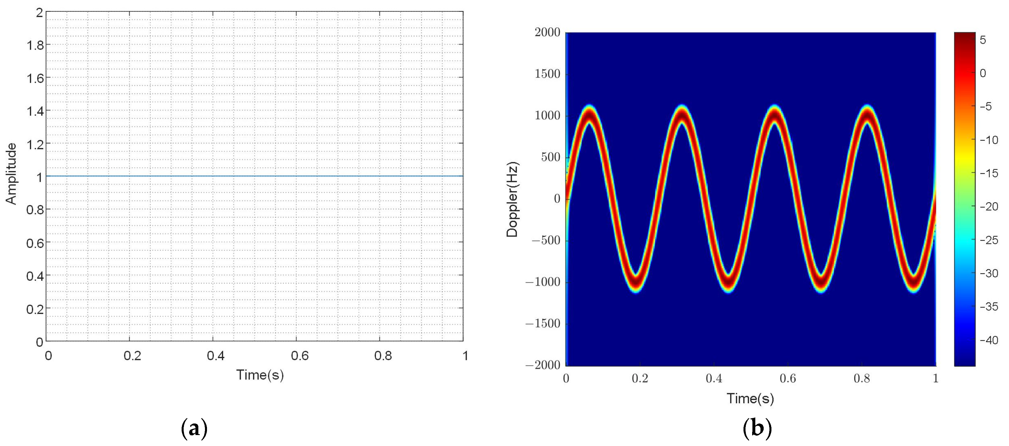
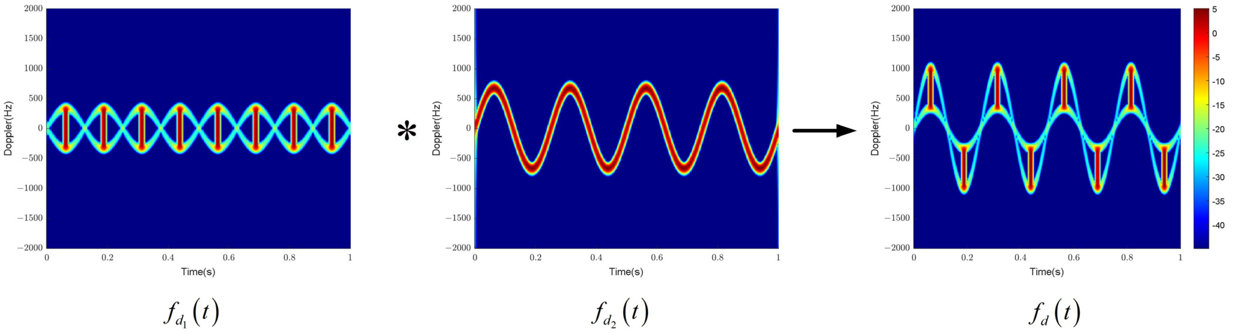
Equation (12) indicates that the frequency domain will contain two distinct frequency components, one of which is time-modulated and the other of which is a constant frequency with a value of zero. It will manifest in the time–frequency domain as a time-modulated sine curve (sine-modulated component) with amplitude $4\pi f_{rot}l\cos \beta \backslash \lambda$ and a direct current line with zero frequency (DC component).

Scenario 2:

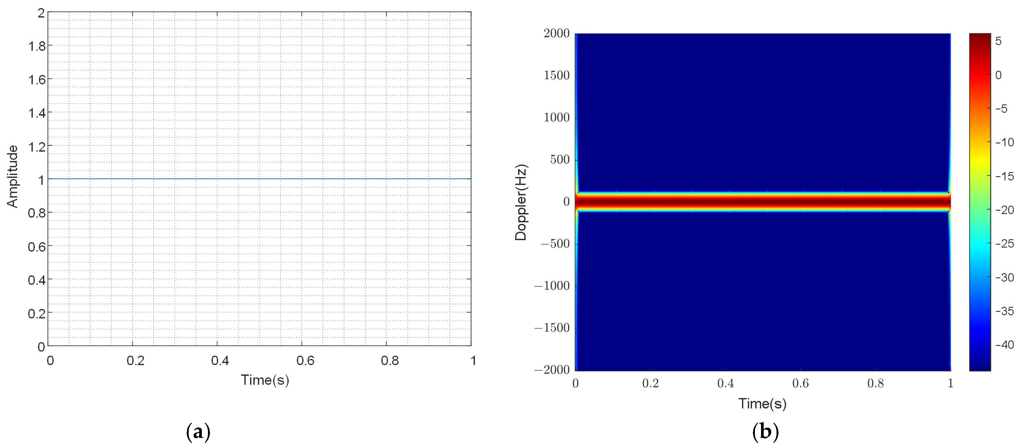
When ${\theta }_1+2\pi f_{rot}t\ne \pi /2+k\pi$, $k=1,2,3,\dots$, $\cos \left({\theta }_1+2\pi f_{rot}t\right)=0$, integrating the echo of all scattering points is impossible. The phase term remains constant and does not influence the amplitude of the signal when only this instant is considered. The current value of the amplitude of the blade echo is as follows:

$$A\left(t\right)=\sigma K.$$

(13)

At this time, the amplitude of the blade echo is determined by the number of scattering points, while its Doppler frequency value is given by the following:

$$\begin{array}{ll}{f}_d\left(t\right)& ={\displaystyle \sum _{i=1}^K\left|f_{d{P}_i}\left(t\right)\right|}\\ & ={\displaystyle \sum _{i=1}^K\left|\frac{4\pi f_{rot}{x}_i}{\lambda }\sin \left({\theta }_1+2\pi f_{rot}t\right)\cos \beta \exp \left(-j\frac{4\pi R_0}{\lambda }\right)\cdot \exp \left(-j\frac{4\pi }{\lambda }\left(x_i\cos \left({\theta }_1+2\pi f_{rot}t\right)\cos \beta \right)\right)\right|}\\ & ={\displaystyle \sum _{i=1}^K\frac{4\pi f_{rot}(i-1)d}{\lambda }\cos \beta }\end{array}.$$

(14)

The frequency of scattering points $P_i$ on the blade is $\left|f_{d{P}_i}\left(t\right)\right|=4\pi f_{rot}(i-1)d\cos \beta /\lambda$, represented in the frequency domain by scattering points that are equally spaced and have identical intensities. It appears to be in the frequency band of the range $\left[0,4\pi f_{rot}l/\lambda \right]$ as the scattering point interval $d$ approaches zero; this phenomenon is known as the time–frequency domain flash.

In the following two scenarios, it is established that the amplitude component of the blade echo can be consistently denoted as follows:

$$A\left(t\right)=\sigma K\cdot \mathrm{sinc}\left({\displaystyle \frac{2l}{\lambda }}\cos \left({\theta }_1+2\pi f_{rot}t\right)\cos \beta \right).$$

(15)

Equation (16) shows that the blade echo exhibits an instantaneous Doppler frequency value as follows:

$$f_d\left(t\right)=\left\{\begin{array}{c}\begin{array}{cc}{\displaystyle \frac{4\pi f_{rot}l}{\lambda }}\sin \left({\theta }_1+2\pi f_{rot}t\right)\cos \beta (\mathrm{Modulated}), 0(\mathrm{DC})& , {\theta }_1+2\pi f_{rot}t\ne {\displaystyle \frac{\pi }{2}}+n\pi \end{array}\\ \begin{array}{cc}{\displaystyle \sum _{i=1}^K\frac{4\pi f_{rot}(i-1)d}{\lambda }\cos \beta \left(\mathrm{Flash}\right)}& , {\theta }_1+2\pi f_{rot}t={\displaystyle \frac{\pi }{2}}+n\pi \end{array}\end{array}\right..$$

(16)

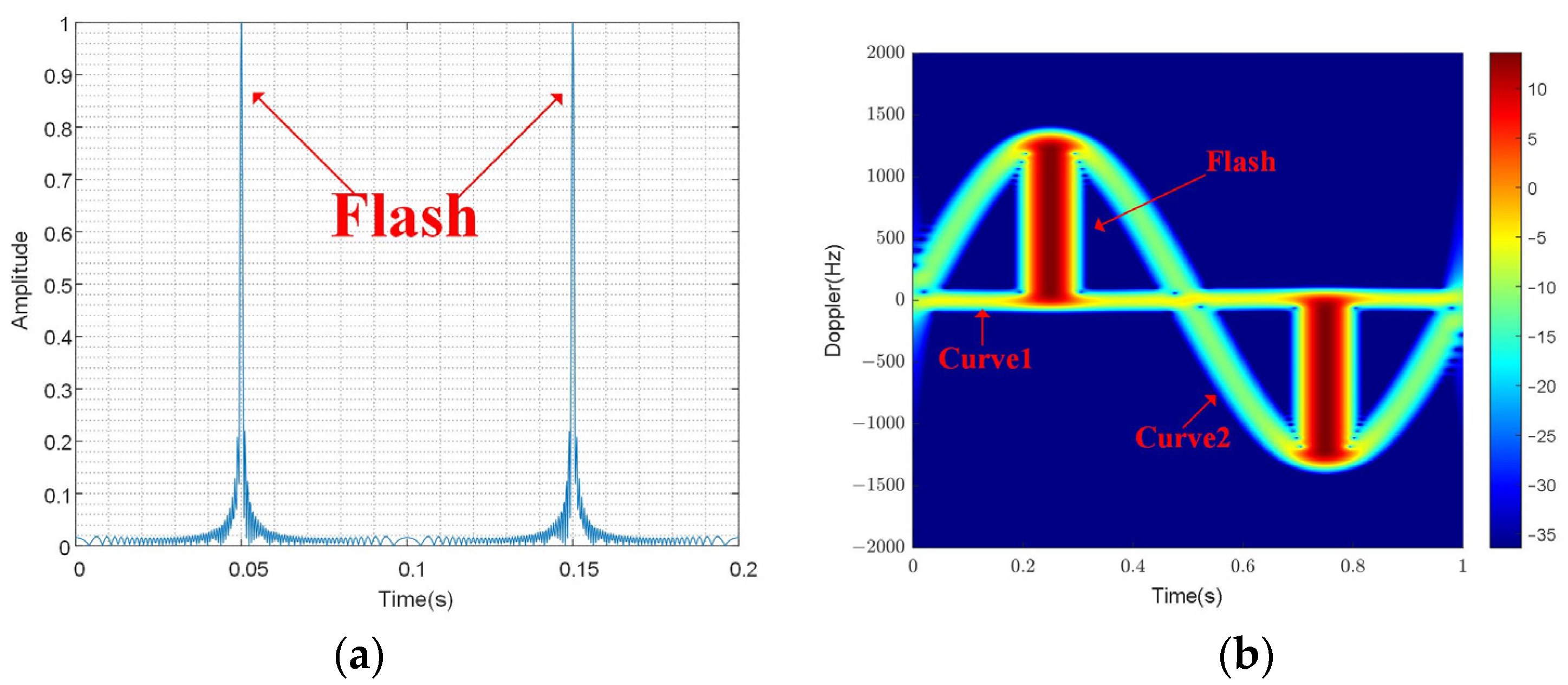
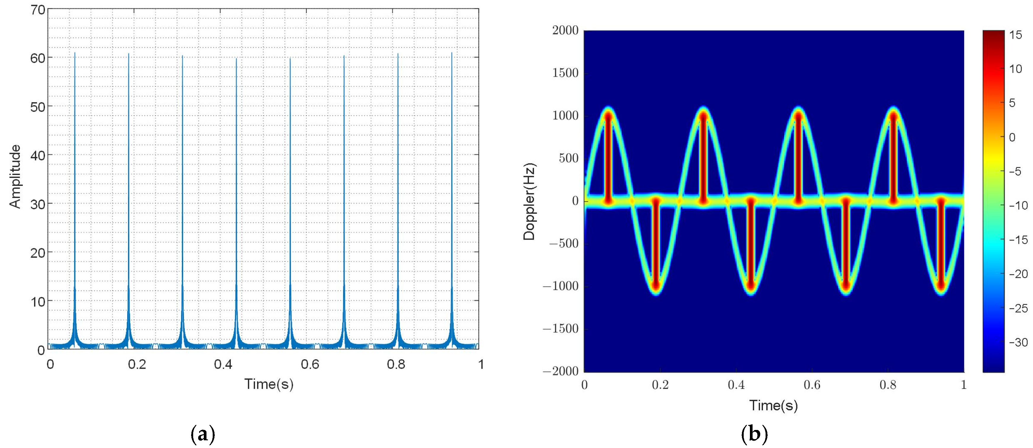
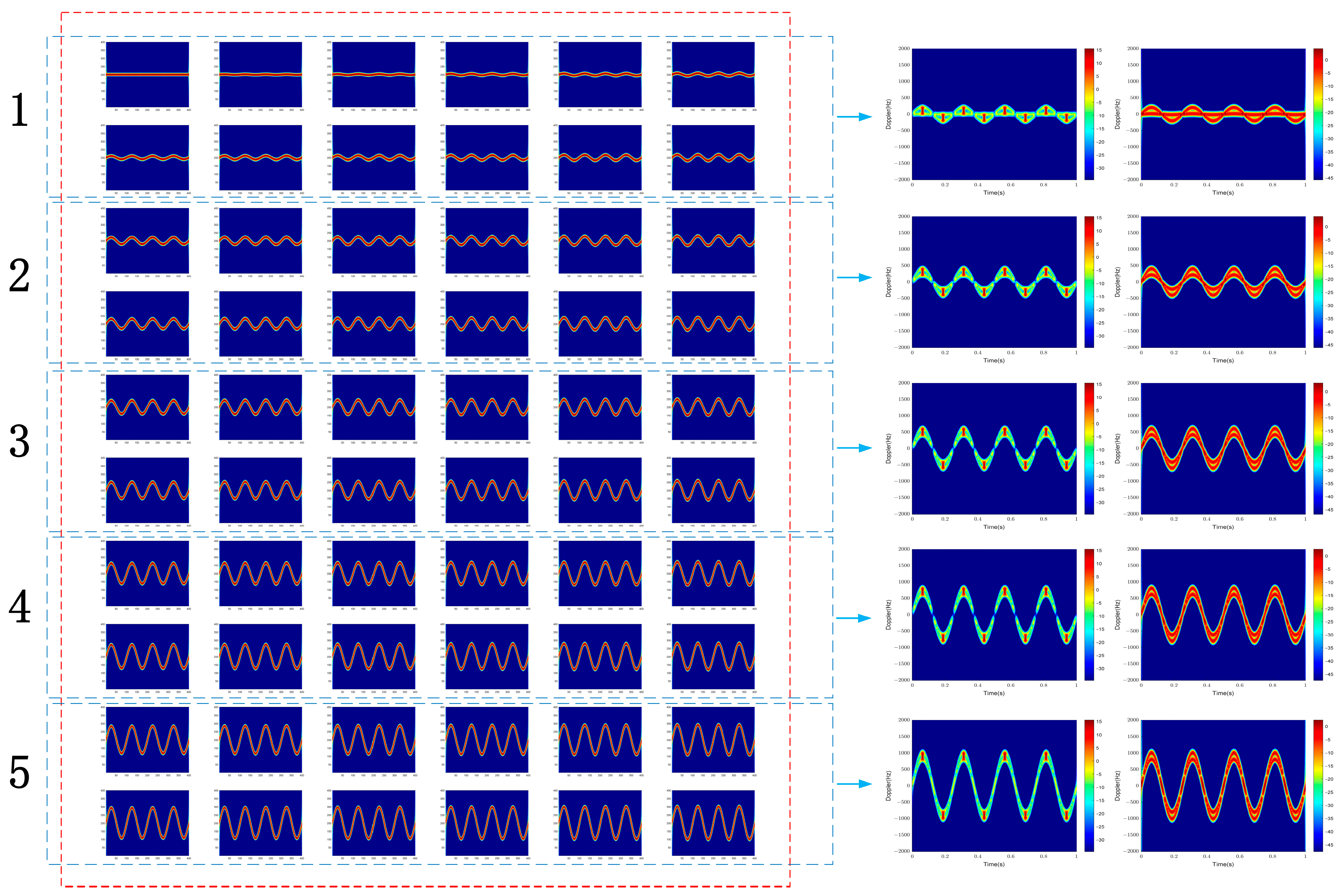
Figure 2 illustrates the time-domain and time–frequency results of the echo. As predicted by the theoretical analysis, the amplitude modulation caused by a $\sin c$ function is consistent with the results in Figure 2. The time–frequency result, which is obtained by taking the derivative of the phase component, illustrates the relationship between time and frequency. Two curves are presented in the time–frequency results: a sine curve with the amplitude at $4\pi f_{rot}l/\lambda$ and a straight line representing the zero-frequency DC component. Simultaneously, when time-domain flash occurs, the frequency band $\left[0,4\pi f_{rot}l/\lambda \right]$ manifests in the time–frequency domain, known as the flash phenomenon in rotor targets.

In Figure 2, the amplitude in the time domain is modulated by the $\mathrm{sinc}$ function, consistent with the theoretical analysis results. The time–frequency results are obtained by short-time Fourier transform (STFT). Short-time Fourier transform (STFT) is usually used to study the time–frequency characteristics of the target echo. This time–frequency transform method is the most direct way to study the time-varying characteristics of signal frequency. This time–frequency transformation method divides the signal into several overlapping blocks, each with its window length, and applies the Fourier transform to the data in each block. This transformation reflects the time–frequency characteristics of the signal frequency. However, its limitation lies in the “window effect” of the transformation, which means that the transformed signal cannot have both high time and high-frequency resolution simultaneously. The choice of window length determines the time resolution and frequency resolution. The longer the window length, the higher the frequency resolution and the lower the time resolution. The shorter the window length, the lower the frequency resolution and the higher the time resolution.

In Equation (17), $s\left(t\right)$ represents the signal, and $w\left(t\right)$ represents the Gaussian window function. In this study, STFT with an appropriate window length 8 achieves suitable time and frequency resolution [19].

$$STFT\left(t,\omega \right)={\displaystyle \int s\left(t^{\prime }\right)}w\left(t^{\prime }-t\right)\exp \left(-j\omega t^{\prime }\right)d{t}^{\prime }$$

(17)

The window function is crucial in the short-time Fourier transform (STFT). Equation (18) shows the Gaussian window function used in this paper.

$$w\left(t\right)={\displaystyle \frac{1}{{\pi }^{1/4}\sqrt{\sigma }}}\exp \left\{-{\displaystyle \frac{t^2}{2{\sigma }^2}}\right\}$$

(18)

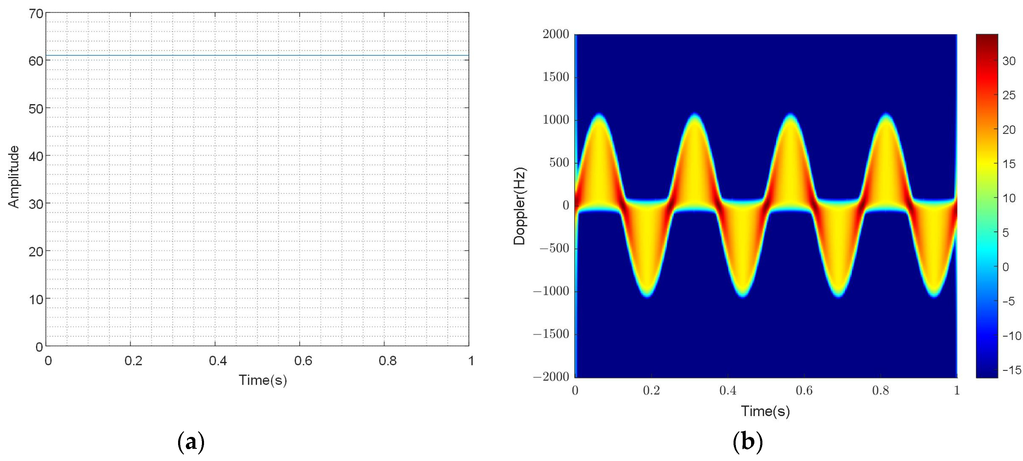
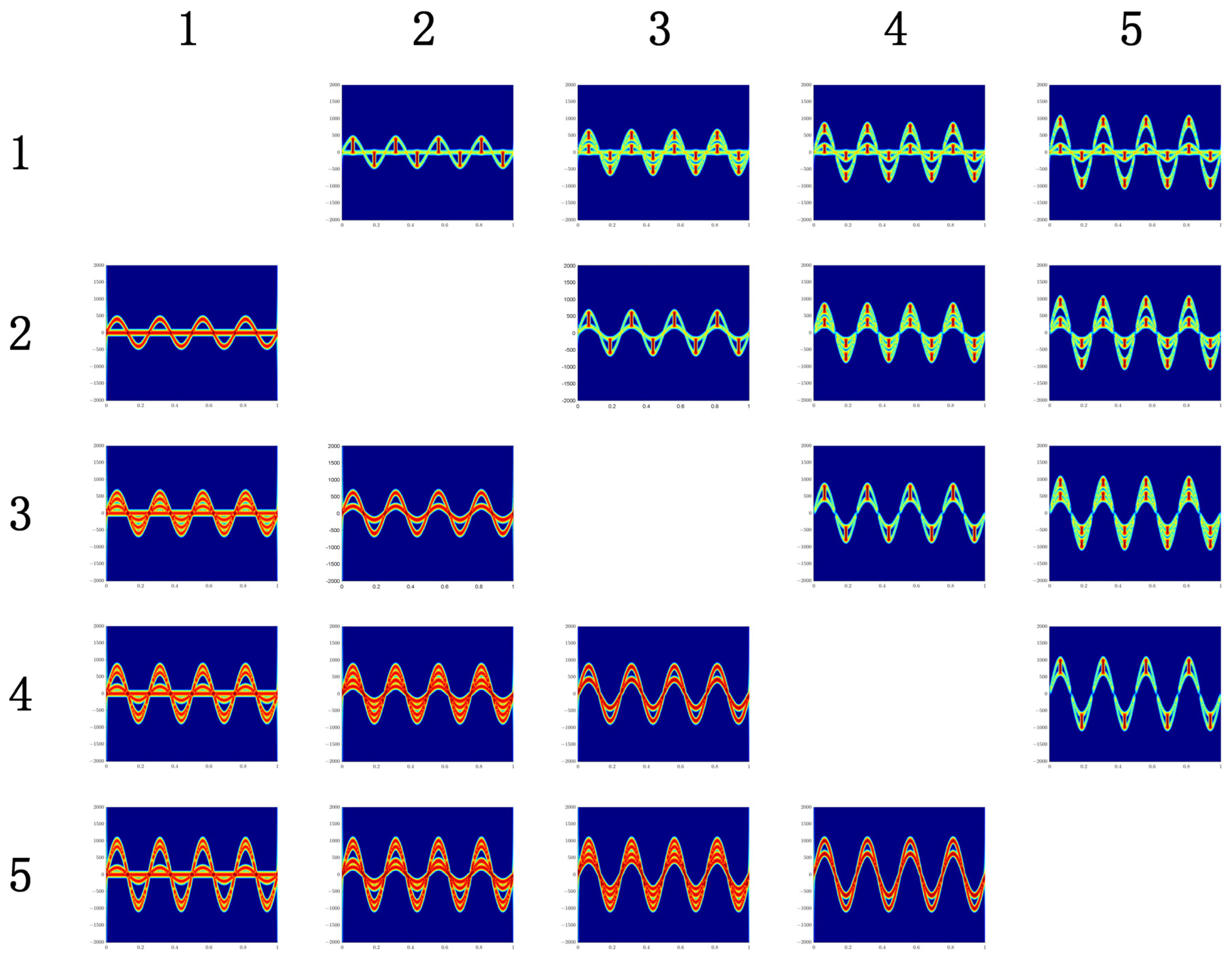
The time–frequency results reflect the relationship between frequency and time, that is, the result of taking the derivative of the phase part. In the time–frequency results, there are two curves, one is a sine curve, and the other is a straight line of the zero-frequency DC component. At the same time, when flash occurs in the time domain, a frequency band $\left[0,4\pi f_{rot}l/\lambda \right]$ also appears in the time–frequency domain, which is called time–frequency domain flash. At this point, there are two curves, a sine curve with an amplitude of $4\pi f_{rot}l/\lambda$ and a sine curve with an amplitude of 0. Due to the frequency being 0, it is easy to ignore when analyzing instantaneous Doppler. Therefore, further theoretical derivation is carried out, assuming that the length of the blade is $l_1-l_2$, $l_1$ is the distance from the outermost scattering point to the center of rotation of the blade, and $l_2$ is the distance from the innermost scattering point to the center of rotation of the blade. The innermost scattering point is not at the origin, which can avoid the case of a frequency of 0. Currently, scenario 2 is divided into scenario 2.1 and scenario 2.2.

Scenario 2.1: When ${\theta }_1+2\pi f_{rot}t=\pi /2+k\pi$, $k=1,2,3,\dots$, the number of scattering points decreases compared to the number of scattering points starting from the origin. At this point, let the number of scattering points be K, and the amplitude of the blade echo is the following:

$$A\left(t\right)=\sigma K_1.$$

(19)

At this moment, the instantaneous Doppler frequency value of the blade echo is the following:

$$\begin{array}{ll}{f}_d\left(t\right)& ={\displaystyle \sum _{i=1}^{K_1}\left|f_{d{P}_i}\left(t\right)\right|}\\ & ={\displaystyle \sum _{i=1}^{K_1}\left|\frac{4\pi f_{rot}{x}_i}{\lambda }\sin \left({\theta }_1+2\pi f_{rot}t\right)\cos \beta \exp \left(-j\frac{4\pi R_0}{\lambda }\right)\cdot \exp \left(-j\frac{4\pi }{\lambda }\left(x_i\cos \left({\theta }_1+2\pi f_{rot}t\right)\cos \beta \right)\right)\right|}\\ & ={\displaystyle \sum _{i=1}^{K_1}\frac{4\pi f_{rot}((i-1)d+l_2)}{\lambda }\cos \beta }\end{array}.$$

(20)

In the frequency domain, the frequency of scattering point $P_i$ on the blade is as follows:

$$\left|f_{d{P}_i}\left(t\right)\right|=4\pi f_{rot}(i-1)d\cos \beta /\lambda ,$$

(21)

where it is manifested as equally spaced scattering points with the same intensity. When $d$ approaches 0, it appears to be within the frequency band of $\left[4\pi f_{rot}{l}_2/\lambda ,4\pi f_{rot}{l}_1/\lambda \right]$, and the flash range in the time–frequency domain changes.

Scenario 2.2: When ${\theta }_1+2\pi f_{rot}t=\pi /2+k\pi$, $k=1,2,3,\dots$, and $\cos \left({\theta }_1+2\pi f_{rot}t\right)\ne 0$, there is a proportional relationship between the phase parts of each scattering point, which can be integrated. The signal can be transformed at this point, as shown in Equation (22).

$$\begin{array}{ll}s\left(t\right)& ={\displaystyle \sum _{i=1}^{K_1}{s}_{P_i}\left(t\right)}=\underset{\mathrm{A} \mathrm{part}}{\underbrace{\sigma K_1}}\underset{\mathrm{B} \mathrm{part}}{\underbrace{{\displaystyle {\int }_{l_1}^{l_2}\exp \left(-j\frac{4\pi R_0}{\lambda }\right)\exp \left(-j\frac{4\pi }{\lambda }\left(x\cos \left({\theta }_1+2\pi f_{rot}t\right)\cos \beta \right)\right)dx}}}\\ & =\underset{\mathrm{A} \mathrm{part}}{\underbrace{{\displaystyle \frac{(l_1-l_2)}{l}}\sigma K}}\underset{\mathrm{B} \mathrm{part}}{\underbrace{{\left.{\displaystyle \frac{\exp \left(-j\frac{4\pi R_0}{\lambda }\right)\exp \left(-j\frac{4\pi }{\lambda }\left(x\cos \left({\theta }_1+2\pi f_{rot}t\right)\cos \beta \right)\right)}{-j\frac{4\pi }{\lambda }\cos \left({\theta }_1+2\pi f_{rot}t\right)\cos \beta }}\right|}_{l_1}^{l_2}}}\\ & =\underset{\mathrm{A} \mathrm{part}}{\underbrace{{\displaystyle \frac{(l_1-l_2)}{l}}\sigma K}}\underset{\mathrm{B} \mathrm{part}}{\underbrace{{\displaystyle \frac{\exp \left(-j\frac{4\pi R_0}{\lambda }\right)(\exp \left(-j\frac{4\pi }{\lambda }\left(l_1\cos \left({\theta }_1+2\pi f_{rot}t\right)\cos \beta \right)\right)-\exp \left(-j\frac{4\pi }{\lambda }\left(l_2\cos \left({\theta }_1+2\pi f_{rot}t\right)\cos \beta \right)\right))}{-j\frac{4\pi }{\lambda }\cos \left({\theta }_1+2\pi f_{rot}t\right)\cos \beta }}}}\\ & =\underset{\mathrm{A} \mathrm{part}}{\underbrace{{\displaystyle \frac{(l_1-l_2)}{l}}\sigma K}}\cdot \underset{\mathrm{B} \mathrm{part}}{\underbrace{{\displaystyle \frac{\exp \left(-j\frac{4\pi R_0}{\lambda }\right)\exp \left(-j\frac{2\pi }{\lambda }\left((l_1+l_2)\cos \left({\theta }_1+2\pi f_{rot}t\right)\cos \beta \right)\right)(\exp \left(-j\frac{2\pi }{\lambda }\left((l_1-l_2)\cos \left({\theta }_1+2\pi f_{rot}t\right)\cos \beta \right)\right)-\exp \left(j\frac{2\pi }{\lambda }\left((l_1-l_2)\cos \left({\theta }_1+2\pi f_{rot}t\right)\cos \beta \right)\right))}{-j\frac{4\pi }{\lambda }\cos \left({\theta }_1+2\pi f_{rot}t\right)\cos \beta }}}}\\ & =\underset{\mathrm{A} \mathrm{part}}{\underbrace{{\displaystyle \frac{(l_1-l_2)}{l}}\sigma K}}\underset{\mathrm{B} \mathrm{part}}{\underbrace{{\displaystyle \frac{\exp \left(-j\frac{4\pi R_0}{\lambda }\right)\exp \left(-j\frac{2\pi }{\lambda }\left((l_1+l_2)\cos \left({\theta }_1+2\pi f_{rot}t\right)\cos \beta \right)\right)\cdot -2j\sin (\frac{2\pi }{\lambda }\left((l_1-l_2)\cos \left({\theta }_1+2\pi f_{rot}t\right)\cos \beta \right))}{-j\frac{4\pi }{\lambda }\cos \left({\theta }_1+2\pi f_{rot}t\right)\cos \beta }}}}\\ & =\underset{\mathrm{A} \mathrm{part}}{\underbrace{{\displaystyle \frac{(l_1-l_2)}{l}}\sigma K}}\underset{\mathrm{B} \mathrm{part}}{\underbrace{\exp \left(-j{\displaystyle \frac{4\pi }{\lambda }}{R}_0\right)\exp \left[-j{\displaystyle \frac{2\pi (l_1+l_2)}{\lambda }}\cos \left({\theta }_1+2\pi f_{rot}t\right)\cos \beta \right]\cdot \mathrm{sinc}\left({\displaystyle \frac{2(l_1-l_2)}{\lambda }}\cos \left({\theta }_1+2\pi f_{rot}t\right)\cos \beta \right)}}\\ & =\underset{\mathrm{A} \mathrm{part}}{\underbrace{{\displaystyle \frac{(l_1-l_2)}{l}}\sigma K\cdot \mathrm{sinc}\left({\displaystyle \frac{2(l_1-l_2)}{\lambda }}\cos \left({\theta }_1+2\pi f_{rot}t\right)\cos \beta \right)}}\underset{\mathrm{B} \mathrm{part}}{\underbrace{\exp \left(-j{\displaystyle \frac{4\pi }{\lambda }}{R}_0\right)\exp \left[-j{\displaystyle \frac{2\pi (l_1+l_2)}{\lambda }}\cos \left({\theta }_1+2\pi f_{rot}t\right)\cos \beta \right]}}\end{array}$$

(22)

In the time domain, the signal amplitude decreases and becomes the original. The phase part is divided into two parts in the time domain, as shown as follows in Equations (23) and (24):

$$\begin{array}{ll}{s}_{d_1}\left(t\right)& =\mathrm{sinc}\left({\displaystyle \frac{2(l_1-l_2)}{\lambda }}\cos \left({\theta }_1+2\pi f_{rot}t\right)\cos \beta \right)\\ & ={\displaystyle \frac{j\exp \left(-j\frac{2\pi (l_1-l_2)}{\lambda }\cos \left({\theta }_1+2\pi f_{rot}t\right)\cos \beta \right)-j\exp \left(j\frac{2\pi (l_1-l_2)}{\lambda }\cos \left({\theta }_1+2\pi f_{rot}t\right)\cos \beta \right)}{\frac{4\pi (l_1-l_2)}{\lambda }\cos \left({\theta }_1+2\pi f_{rot}t\right)\cos \beta }}\end{array},$$

(23)

$$s_{d_2}\left(t\right)=\exp \left(-j{\displaystyle \frac{4\pi }{\lambda }}{R}_0\right)\exp \left[-j{\displaystyle \frac{2\pi (l_1+l_2)}{\lambda }}\cos \left({\theta }_1+2\pi f_{rot}t\right)\cos \beta \right].$$

(24)

For the first part $s_{d_1}\left(t\right)$, when the denominator is $4\pi (l_1-l_2)\cos \left({\theta }_1+2\pi f_{rot}t\right)\cos \beta /\lambda$ and only $\cos \left({\theta }_1+2\pi f_{rot}t\right)\cos \beta =0$, it impacts the instantaneous Doppler frequency of the signal. At other times, it only exhibits broadening (or compression) in the frequency domain. The instantaneous Doppler frequency can be seen as the phase derivative of the two single components in the middle, as shown in Equation (25). For the second part, the phase can be directly differentiated, as shown in Equation (26):

$$\begin{array}{ll}{f}_{d_1}\left(t\right)& =\left[{\displaystyle \frac{1}{2\pi }}{\displaystyle \frac{d\frac{2\pi (l_1-l_2)}{\lambda }\cos \left({\theta }_1+2\pi f_{rot}t\right)\cos \beta }{dt}},-{\displaystyle \frac{1}{2\pi }}{\displaystyle \frac{d\frac{2\pi (l_1-l_2)}{\lambda }\cos \left({\theta }_1+2\pi f_{rot}t\right)\cos \beta }{dt}}\right]\\ & =\left[{\displaystyle \frac{2\pi f_{rot}(l_1-l_2)}{\lambda }}\sin \left({\theta }_1+2\pi f_{rot}t\right)\cos \beta ,-{\displaystyle \frac{2\pi f_{rot}(l_1-l_2)}{\lambda }}\sin \left({\theta }_1+2\pi f_{rot}t\right)\cos \beta \right]\end{array},$$

(25)

$$f_{d_2}\left(t\right)={\displaystyle \frac{1}{2\pi }}{\displaystyle \frac{d\varphi (t)}{dt}}={\displaystyle \frac{d-\frac{2\pi (l_1+l_2)}{\lambda }\cos \left({\theta }_1+2\pi f_{rot}t\right)\cos \beta }{dt}}={\displaystyle \frac{2\pi f_{rot}(l_1+l_2)}{\lambda }}\sin \left({\theta }_1+2\pi f_{rot}t\right)\cos \beta .$$

(26)

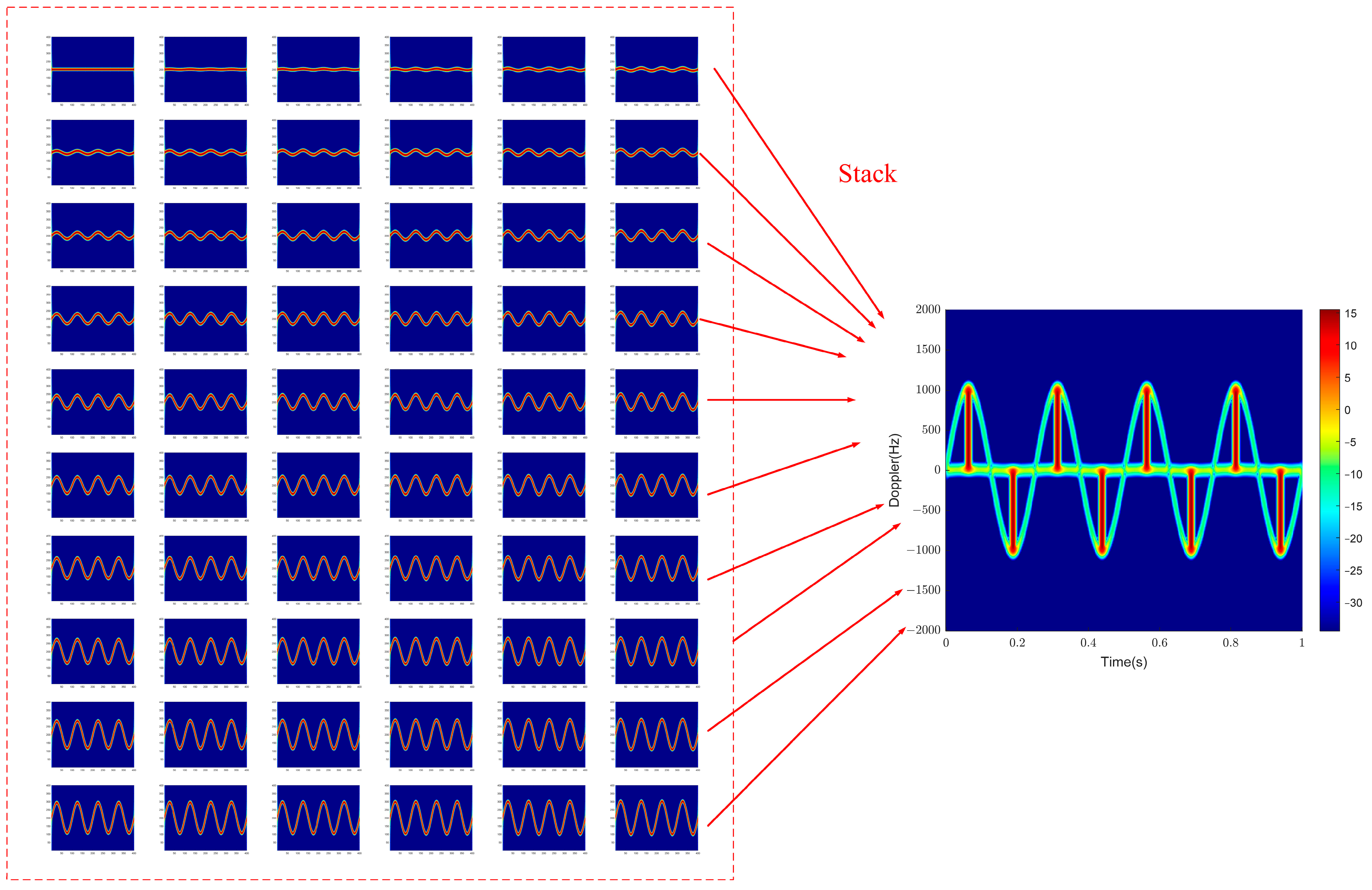
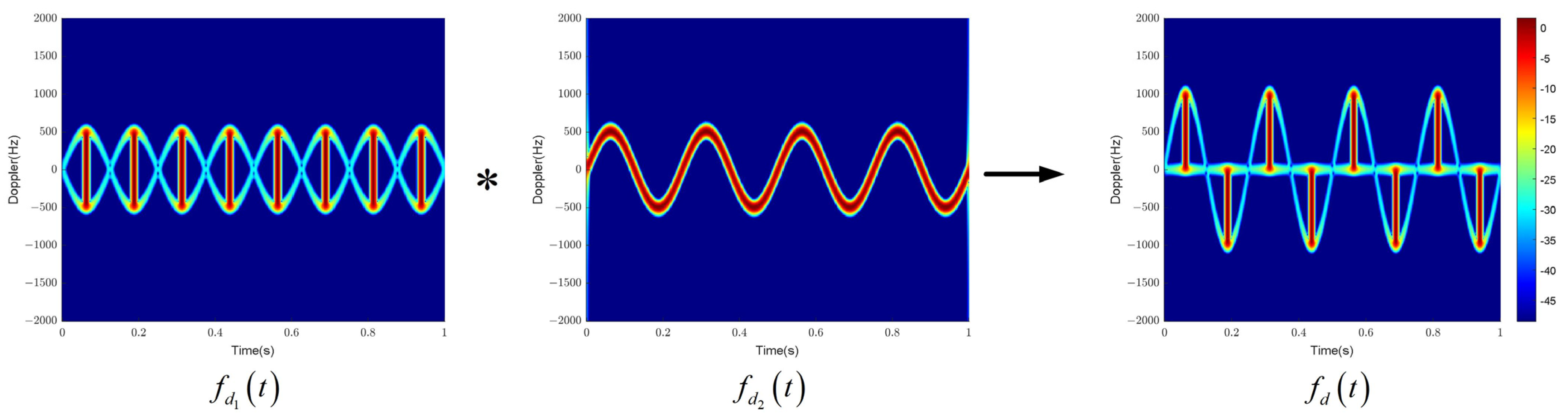
At this point, we convolve the instantaneous Doppler frequencies of the two parts as follows:

$$\begin{array}{ll}{f}_d\left(t\right)& =f_{d_1}\left(t\right)\ast f_{d_2}\left(t\right)\\ & =\left[{\displaystyle \frac{2\pi f_{rot}(l_1-l_2)}{\lambda }}\sin \left({\theta }_1+2\pi f_{rot}t\right)\cos \beta ,-{\displaystyle \frac{2\pi f_{rot}(l_1-l_2)}{\lambda }}\sin \left({\theta }_1+2\pi f_{rot}t\right)\cos \beta \right]\ast {\displaystyle \frac{2\pi f_{rot}(l_1+l_2)}{\lambda }}\sin \left({\theta }_1+2\pi f_{rot}t\right)\cos \beta \\ & =\left[{\displaystyle \frac{4\pi f_{rot}{l}_1}{\lambda }}\sin \left({\theta }_1+2\pi f_{rot}t\right)\cos \beta ,{\displaystyle \frac{4\pi f_{rot}{l}_2}{\lambda }}\sin \left({\theta }_1+2\pi f_{rot}t\right)\cos \beta \right]\end{array}.$$

(27)

According to the results, there are two curves in the time–frequency domain, one with an amplitude of the sine modulation curve and the other with an amplitude of the sine modulation curve. The instantaneous Doppler frequency value of the blade echo is given by the following:

$$f_d\left(t\right)=\left\{\begin{array}{c}\begin{array}{cc}\left[{\displaystyle \frac{4\pi f_{rot}{l}_1}{\lambda }}\cos \left({\theta }_1+2\pi f_{rot}t\right)\cos \beta ,{\displaystyle \frac{4\pi f_{rot}{l}_2}{\lambda }}\cos \left({\theta }_1+2\pi f_{rot}t\right)\cos \beta \right]& ,{\theta }_1+2\pi f_{rot}t\ne {\displaystyle \frac{\pi }{2}}+n\pi \end{array}\\ \begin{array}{cc}{\displaystyle \sum _{i=1}^K\frac{4\pi f_{rot}((i-1)d+l_2)}{\lambda }\cos \beta }& ,{\theta }_1+2\pi f_{rot}t={\displaystyle \frac{\pi }{2}}+n\pi \end{array}\end{array}.\right.$$

(28)

3. Experiment Analysis

A rotor blade is taken as the object based on theoretical analysis, and an equally spaced scattering point echo model is used for simulation experiments. We set the length of the blade to 6 m, the spacing between scattering points to 0.1 m, and the number of blades to 1 for simulation. The consistency of the fundamental parameters in the simulation is illustrated in

Table 1. Fundamental parameters in the simulation.

Parameters	σ	frot/Hz	θ1/°	The Position of the Radar	λ/m	PRF/Hz	T/s	The Relationship Between Radar and Rotor Blade Position
								$\mathit{R}$/m	β/°	α/°
Value	1	4	0	(0,0,0)	0.3	4000	1	50,000	0	0

. For time–frequency analysis of the simulation, STFT with a Gaussian window as the window function [20] is utilized. Two different scenarios are discussed in simulation.

3.1. The Simulation Results of a Single Scattering Point Compared with All Scattering Points

The results of the outermost scattering point and the innermost scattering point are simulated. Figure 3 shows the time-domain and time–frequency results of the echo, and the time-domain and time–frequency results of the echo are shown in Figure 4.

Figure 3 and Figure 4 show that for each scattering point, the amplitude of the echo results in the time domain is constant (scattering coefficient). Its instantaneous Doppler frequency is sinusoidally modulated by time in the frequency domain. Overlaying the echoes from the outermost scattering point and the innermost scattering point, Figure 5 shows the time-domain and frequency-domain results of the echoes.

As shown in Figure 5, when each scattering point is stacked, the amplitude of the echo result will change in the time domain due to interference between the two scattering points, and it will also impact the frequency domain. The frequency domain’s impact is insignificant when the scattering points are discontinuous. Further, all scattering point simulations will be studied, and all scattering points will be taken.

The echoes of each scattering point are stacked. Figure 6 illustrates the stacking procedure, wherein each scattering point echo is subjected to a time–frequency transformation to generate the corresponding time–frequency results. The final time–frequency results are then obtained by stacking each time–frequency result. The results for the time and time–frequency domains are illustrated in Figure 7.

The presence of interference between every scattering point is evident in Figure 6. Following stacking, the signal amplitude is modulated in the time domain. Close connections exist between each scattering point in the frequency domain. Flashing will ensue in the time–frequency domain when a peak is observed in the time domain. At other moments, the time–frequency domain comprises solely the time–frequency results originating from the innermost and exterior scattering points.

From Figure 6 and Figure 7, it can be seen that there is “interference” between each scattering point. In the time domain, the signal’s amplitude is modulated by a function after superposition. In the frequency domain, the connections between each scattering point are close. When a peak appears in the time domain, the flash will occur in the time–frequency domain. At other times, the time–frequency domain comprises the time–frequency results of the outermost and innermost scattering points (origin). Further, to verify whether there is interference between each scattering point and in the time domain, the echoes of each scattering point are added by taking the mode. In the time–frequency domain, the time–frequency results of each scattering point are added after taking the mode, as shown in Figure 8.

Figure 8 shows that if the modes of each scattering point are taken and added together, the phase relationship between the time domain and time–frequency domain will be removed. At this time, the time domain is not affected by the phase, and the amplitude is the cumulative result of each scattering point. In the time–frequency domain, the sine modulation curves of each scattering point in the time–frequency domain are superimposed. At this time, the scattering points do not affect each other, and the sine modulation curves of each scattering point only have different amplitudes. Therefore, Figure 8b shows the results after superposition. The part between the sine modulation curve of the outermost scattering point and the sine modulation curve of the innermost scattering point is covered by the sine modulation curve of the scattering point.

3.2. The Phase Part Simulation Results

As shown in Figure 9, the time–frequency results of the echo on the two parts of the phase are obtained after STFT, that is $f_{d_1}\left(t\right),f_{d_2}\left(t\right)$, the relationship between instantaneous Doppler frequency and time. Figure 9 shows the time–frequency results obtained by convolving the time–frequency results of the phase two parts of the blade length from the origin to the outermost scattering point and the time–frequency results of these two parts.

In Figure 9, the time–frequency results of $f_{d_1}\left(t\right)$ consist of two sine curves with an amplitude of $2\pi f_{rot}l\cos \beta /\lambda$ that are symmetrical about the $x$ axis. The flash in the sine curve because the moment of the flash is nondifferentiable. Each scattering point has frequency values, and there is no interference in the frequency part. The frequency components are staked from each scattering point component. The time–frequency results of $f_{d_2}\left(t\right)$ is a sine curve with an amplitude of $2\pi f_{rot}l\cos \beta /\lambda$. The final time–frequency results are obtained by combining the time–frequency results of the two components. Upon comparing the obtained time–frequency results from stacking the scattering points with the theoretical analysis, it is evident that the results stay consistent.

Figure 10 shows the time–frequency results of the two parts of the phase from the innermost scattering point (no origin) to the farthest scattering point of the blade length and the time–frequency results of the two parts after convolution. Some of the time–frequency results are two symmetric sine curves about the origin with an amplitude of 750, and some of the time–frequency results become a sine curve with an amplitude of 1200, consistent with theoretical analysis.

3.3. All Scattering Points Divide into Groups

Some scattering points are taken, and the time–frequency results of their echoes are superimposed. Figure 11 shows the stacking process and results. We take the first 60 scattering points, with every 12 scattering points as a group, and superimpose the time–frequency results of this group of scattering points. Figure 9 shows the superimposed time–frequency results. There are also corresponding time–frequency results on the right side of the superimposed results. This result corresponds to the time–frequency results obtained by superimposing the time–frequency results of the innermost scattering points and the outermost scattering points in a group. Through comparison, after superimposing the time–frequency results of the scattering points, flash occurs at fixed moments, and interference occurs between scattering points at other moments. The sine modulation curves of all scattering points will spread to the innermost and outermost sine modulation curves.

On this basis, the time–frequency results of different groups are superimposed, and Figure 12 shows the superimposed results. From the superimposed time–frequency results, it can be seen that for different groups, if the groups are adjacent, the interference of sinusoidal modulation between adjacent scattering points will expand, causing the flash width in the time–frequency results and the amplitude difference of sinusoidal modulation between the outermost and innermost scattering points to increase; if the groups are not adjacent, the impact between the two groups is not significant.

In the two scenarios, the analysis of simulation results thoroughly explains the flash phenomenon in rotor targets. The flash phenomenon in rotor targets is formed due to interference between scattering points in rotor targets.

4. Conclusions

This paper presented a methodical examination of the flash phenomenon on rotor targets. Based on the scattering coefficient of scattering points and the distribution of scattering points on the blade, a scattering point echo model of rotor blades was constructed. On this basis, the influence of each scattering point on the echo was analyzed, and the mechanism of the flash phenomenon was thoroughly analyzed, starting from the analytical expression of the echo. The flash phenomenon was investigated within the domains of time and frequency. The simulation results indicate that the flash phenomenon observed in rotor targets can be attributed to the interference between scattering points. This interference significantly impacts both the temporal and spectral characteristics of the target. The subsequent phase of this research will rely on the theory proposed, aiming to leverage the flash attributes of rotor targets to accomplish tasks such as identifying and detecting rotor targets.