Online Three-Dimensional Fuzzy Reinforcement Learning Modeling for Nonlinear Distributed Parameter Systems

Abstract

Distributed parameter systems (DPSs) frequently appear in industrial manufacturing processes, with complex characteristics such as time–space coupling, nonlinearity, infinite dimension, uncertainty and so on, which is full of challenges to the modeling of the system. At present, most DPS modeling methods are offline. When the internal parameters or external environment of DPS change, the offline model is incapable of accurately representing the dynamic attributes of the real system. Establishing an online model for DPS that accurately reflects the real-time dynamics of the system is very important. In this paper, the idea of reinforcement learning is creatively integrated into the three-dimensional (3D) fuzzy model and a reinforcement learning-based 3D fuzzy modeling method is proposed. The agent improves the strategy by continuously interacting with the environment, so that the 3D fuzzy model can adaptively establish the online model from scratch. Specifically, this paper combines the deterministic strategy gradient reinforcement learning algorithm based on an actor critic framework with a 3D fuzzy system. The actor function and critic function are represented by two 3D fuzzy systems and the critic function and actor function are updated alternately. The critic function uses a TD (0) target and is updated via the semi-gradient method; the actor function is updated by using the chain derivation rule on the behavior value function and the actor function is the established DPS online model. Since DPS modeling is a continuous problem, this paper proposes a TD (0) target based on average reward, which can effectively realize online modeling. The suggested methodology is implemented on a three-zone rapid thermal chemical vapor deposition reactor system and the simulation results demonstrate the efficacy of the methodology.

1. Introduction

Distributed parameter systems (DPSs) are prevalent in the real world, such as flexible beams [1], transport reaction processes [2] and heat processes [3]. Modeling these systems is crucial for the design, optimization, dynamic prediction and control. However, due to the complex system characters, such as time–space coupling, infinite dimension and so on, it is difficult to model these systems.

In the last several decades, many modeling methods of DPS have been proposed and these methods may be broadly classified into two distinct types. Grey/black box modeling with unknown partial differential equations [4,5,6,7] and first principles modeling with known partial differential equations (PDEs) [8,9,10,11,12,13] are the two types of modeling. Obtaining an accurate mathematical description of a system using partial differential equations is challenging due to imperfect understanding of physical and chemical processes. Compared with the first principles modeling method, the grey/black box modeling method is used more widely in practice. This study concentrates on the black box modeling method, which involves developing a model for a DPS without knowledge of the system’s partial differential equation structure or its parameters.

The black box modeling method drives a model for the DPSs in a data-driven style [14]. To date, the most common data-driven modeling methods [15,16,17,18] of DPSs are based on KL decomposition, such as KL-MLP-LSTM [19], in which the infinite dimensional spatiotemporal coupling data are reduced to finite dimensional by KL decomposition, and the space base function is extracted from it, then the time series model is constructed by MLP-LSTM and finally the DPS model is completed by spatiotemporal synthesis. In Ref. [20], two neural network modeling methods are proposed. One is to use the control quantity and position information as the input and the output of the system is the system mathematical model obtained by training the neural network. The other is that singular value decomposition (SVD) is employed to separate the output data of the system in time and space, then a neural network is used to identify the relationship between the control variables and time coefficients and finally the finite low dimensional model of the system is generated via space–time reconstruction. Although the KL decomposition-based methods have been successfully employed in many applications, they neglect the influence of nonlinear space dynamics and depend on model reduction, which can lead to precision loss.

In recent years, a novel DPS modeling method has been developed: three-dimensional (3D) fuzzy modeling [21,22,23]. The preceding and resulting components of a 3D fuzzy system are the temporal coefficient and space base function, respectively. This is a natural implementation of time–space separation and time–space reconstruction. The time–space separation is achieved through the computation of the preceding and resulting components, while the time–space reconstruction is achieved through the union of all activated 3D rules. The 3D fuzzy modeling method has two distinct advantages: linguistic interpretability and a lack of dependence on model reduction. A novel 3D fuzzy modeling framework without model reduction was proposed in Ref. [24], where a 3D fuzzy model is established by employing the nearest neighbor clustering algorithm, the similarity analysis and multiple support vector regression. The method described in Reference [25] employed spatial multiple output support vector regression (MSVR) to construct a comprehensive 3D fuzzy rule foundation. However, the above methods are offline modeling methods, i.e., historical data-driven models. As the internal or external parameters of a distributed parameters system change over time, the performance of the offline model will become worse and worse [26].

Therefore, DPS online modeling has become a research hotspot recently. In Ref. [27], Wang and Li proposed an online modeling method based on incremental spatiotemporal learning. The methods of incremental learning iteratively update the space base function and the accompanying temporal model. In reference [28], Lu et al. introduced a nonlinear time-varying support vector machine model that depended on a spatiotemporal linear support vector machine. This model combined the adaptable space kernel functions with an online time factor model to reconstruct the DPS system. However, those online modeling methods have a complex modeling process and lack language interpretability.

Compared to the traditional learning methods, the reinforcement learning-based methods are naturally implemented in an incremental way based on immediate rewards obtained during the interaction, enabling online learning for different tasks. Reinforcement learning, as a very active algorithm in the field of machine learning, has been used in many disciplines like [29], control [30,31], recognition [32], batching [33], scheduling [34] and optimization [35,36]. Reinforcement learning algorithms learn the optimal policy directly from interactions with the environment, i.e., DPS in this paper. The fundamental components of reinforcement learning algorithms include policy, reward function, value function and environment.

Reinforcement learning algorithms may be categorized into two main types: value function-based reinforcement learning and direct policy search-based reinforcement learning, depending on the methodologies of policy updating and learning [37]. For value function-based reinforcement learning algorithms, David Sliver proposed DQN (Deep Q-network) [38] by combining deep neural network with reinforcement learning. There is also FQ-learning [39] which combines a custom fuzzy system with Q-learning. As for direct policy search-based reinforcement learning, David Sliver et al. [33] proposed DPG (deterministic policy gradient) and proved for the first time that a deterministic policy gradient exists. DPG uses a deterministic policy and outputs deterministic actions for each state, so it avoids expectation in the action space and greatly increases the sample utilization.

In recent years, the combination of reinforcement learning (RL) and fuzzy systems has become an important research direction in the field of intelligent control and decision-making systems. This combination aims to leverage the adaptive and self-optimizing capabilities of RL and the advantages of fuzzy systems in handling uncertainty and fuzzy information, thereby creating more intelligent and robust systems. The integration of RL and fuzzy systems, often referred to as fuzzy reinforcement learning (FRL), combines the learning abilities of RL with the rule-based reasoning of fuzzy systems to effectively solve decision-making problems in complex environments. Specifically, fuzzy systems can serve as approximators for RL’s policy functions or value functions, helping agents make smooth decisions in continuous spaces. Additionally, RL can automatically adjust the rules and parameters of fuzzy systems through online learning, thereby enhancing the adaptability and performance of the system. In Reference [40], a fuzzy Q-learning method was proposed to achieve the online tuning of a PID controller. By introducing a fuzzy system, it addresses the issue that the traditional Q-learning algorithm cannot handle continuous state–action spaces. The paper proposed a fuzzy Q-learning multi-agent system algorithm, where three agents were used to control the three variables of the PID controller and experimental results demonstrate the effectiveness of this method. In Reference [41], a method based on fuzzy actor–critic reinforcement learning was proposed to address the tracking problem. By using a fuzzy system, it enhanced the interpretability of network parameters, making the mapping structure easier to trace and understand. Compared with an artificial neural network, a fuzzy system is more explainable and it allowed the incorporation of necessary human knowledge to construct the inference rules. In Reference [42], an Intelligent Traffic Control Decision-Making method based on Type-2 Fuzzy and Reinforcement Learning was proposed. In this method, the output action of the Type-2 fuzzy control system replaced the action of selecting the maximum output Q-value of the target network in the DQN algorithm, reducing the error caused by the max operation in the target network. In Reference [43], a dynamic fuzzy Q-learning method was proposed, which enabled the automatic learning of the structure and parameters of the fuzzy system based on Q-learning. The effectiveness of the proposed method was validated through the wall-following task of mobile robots.

However, there is very little research on applying reinforcement learning and a fuzzy system to modeling distributed parameter systems. As far as we know, Wang Z. et al. [44] introduced a modeling method for DPSs based on reinforcement learning algorithms. The fundamental concept is to represent the arrangement of measurement sensors in the DPS as a Markov Decision Process model and then use a reinforcement learning method based on a value function to ascertain the most advantageous sensor placement. However, this method employs an offline modeling method, meaning that once the sensor positions are determined, they remain fixed. When the dynamic characteristics of the distributed parameter system change, the initially optimal sensor placement may no longer be optimal, resulting in a substantial decrease in the accuracy of the model.

This study introduces a novel reinforcement learning-based method for online 3D fuzzy modeling. Based on the actor–critic framework, using the deterministic strategy gradient theory, two 3D fuzzy systems are used to represent the actor function and the critic function, respectively, and the critic function and actor function are updated alternately. The critic function uses TD (0) target and is updated by the semi-gradient method; the actor function changes via incorporating the chain derivation rule to the behavior value function. The actor function serves as the established DPS online model. Because DPS online modeling is a continuous problem, it has been in progress without termination. Thus, the average reward return is used and the actor can update itself for each data in real time, so as to realize online modeling.

The main contribution are as follows:

• The actor–critic framework is combined with 3D fuzzy systems to construct a novel online 3D modeling method using the deterministic policy gradient reinforcement learning algorithm.
• Three-dimensional fuzzy deterministic policy gradient algorithm with average reward set is proposed to solve the continuing modeling problem of DPS. The chosen reward set is the average rate of reward every time step, which defines the performance.
• This online modeling method has the ability to build an online model adaptively from scratch without human knowledge.

The subsequent sections of this work are structured in the following manner. Section 2 outlines the concept of the DPS modeling issue. Section 3 provides a comprehensive description of the suggested method for modeling a 3D fuzzy system using reinforcement learning in an online setting. The suggested modeling technique is used in a rapid thermal chemical vapor deposition system and the outcome of the experiment is shown in Section 4. Section 5 provides the final conclusion.

2. Problem Formulation

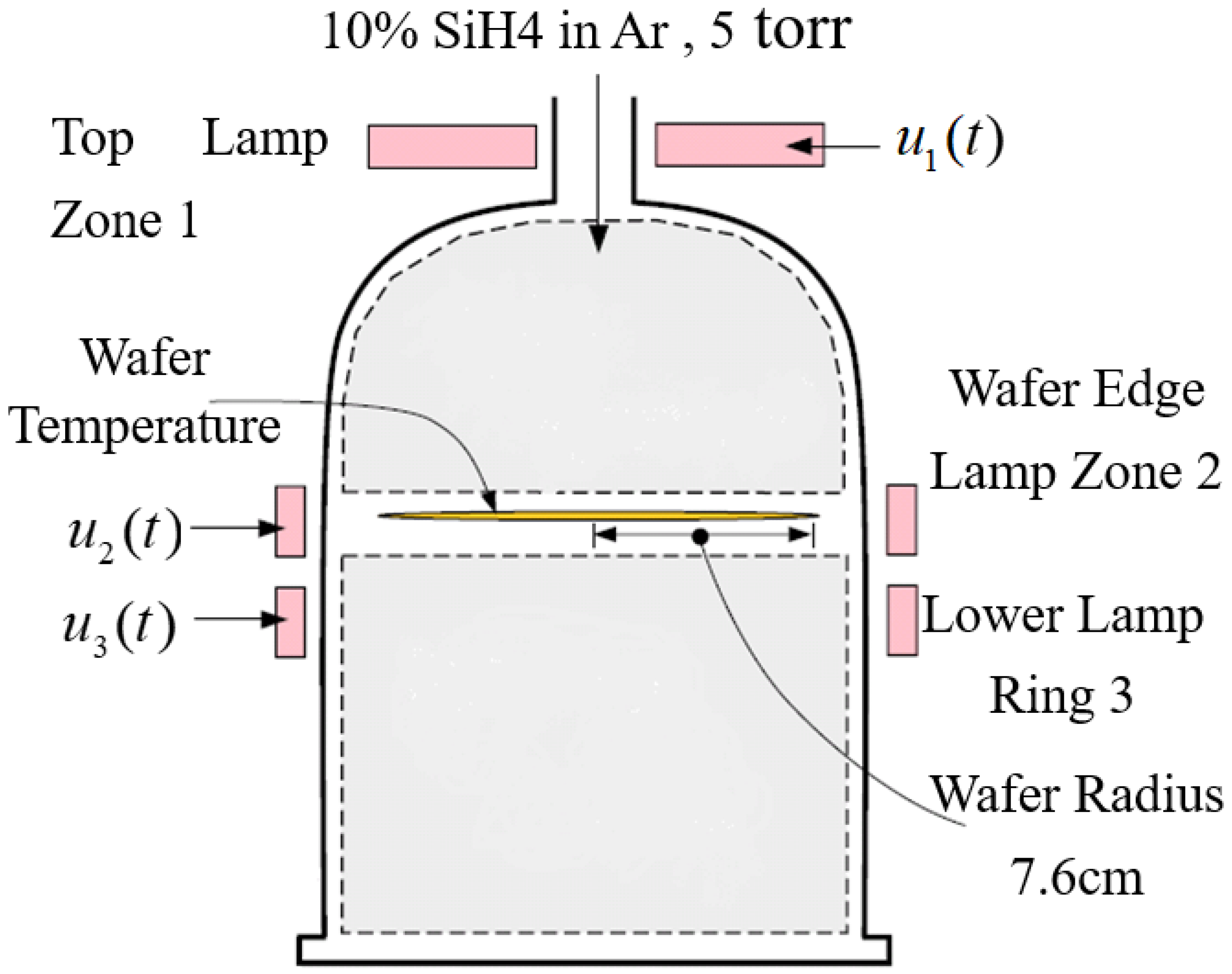
DPS commonly appears in industrial manufacturing processes. Taking the rapid thermal chemical vapor deposition (RTCVD) system in the semiconductor industry as an example, we introduce the characteristics and mathematical description of a DPS.

Figure 1 displays the schematic of an RTCVD system. A 6-inch silicon wafer is placed on a rotating platform inside the chamber of the system and exposed to heat from a heating apparatus. There are three lamp banks that make up the heating system. The first lamp bank warms the wafer’s surface evenly. The second lamp bank heats only the wafer’s edges and the third lamp bank warms the wafer evenly all over. Figure 2 shows the heating lamps’ output incident radiation flux. The reactor is fed 10% concentration of silane gas ($Si{H}_4$). After breaking down, SiH4 yields silicon ($Si$) and hydrogen gas ($H_2$). After about one minute, the wafer is covered with a 0.5 $\mathsf{\mu }$m thick layer of polysilicon that has been deposited at temperatures of at least 800K. The support is rotated to ensure that the temperature is distributed evenly in the azimuthal direction when the wafer is processing. Because the wafer is very thin, the temperature change in the $Z-axis$ direction is ignored. Therefore, providing a uniform temperature distribution along the length of the wafer radius becomes the decisive factor for depositing a uniform layer of polysilicon on the wafer surface. The uniform distribution of the temperature can be controlled by adjusting the power of the heating lamp group in the three zones. This thermal dynamic characteristic can be described by a one-dimensional spatiotemporal coupled PDE model, as follows:

$$\begin{array}{ccc}\hfill & 𝜕T_f^{\prime }/𝜕t^{\prime }=k_0[(1/f^{\prime })𝜕T_f^{\prime }/𝜕f^{\prime }+{𝜕}^2{T}_f^{\prime }/𝜕{f^{\prime }}^2]+{\sigma }_0(1-{T_f^{\prime }}^4)+w_f{q}_1\left(f^{\prime }\right)u_1+w_f{q}_2\left(r^{\prime }\right)u_2\hfill & \hfill +w_f{q}_3\left(r^{\prime }\right)u_3\end{array}$$

(1)

The above PDE is constrained by the following boundary conditions:

$$\begin{array}{c}\mathrm{s}.\mathrm{t}.\left\{\begin{array}{cc}{T}_f^{\prime }/𝜕f^{\prime }={\sigma }_{ed}\left(1-{T_f^{\prime }}^4\right)+q_{ed}{u}_b\hfill & \mathrm{when}{f}^{\prime }=1\\ 𝜕T_f^{\prime }/𝜕f^{\prime }=0\hfill & \mathrm{when}{f}^{\prime }=0\end{array}\right.\hfill \end{array}$$

(2)

$T_f^{\prime }$ represents the dimensionless wafer temperature, expressed as $T_f/T_{amb}$. Here, $T_f$ represents the actual wafer temperature and $T_{amb}$ represents the ambient temperature. In this study, $T_{amb}$ = 300K. $t^{\prime }$ represents the dimensionless time, expressed as ${\displaystyle \frac{t}{\tau }}$. Here, t represents the actual time and $\tau$ is 2.9s. $f^{\prime }$ represents the dimensionless radius position, expressed as ${\displaystyle \frac{f}{R_w}}$. Here, f represents the actual radius position and $R_w$ is 7.6 cm. $u_1$, $u_2$ and $u_3$ represent the power of three heating lamp groups, respectively. $q_1\left(f^{\prime }\right)$, $q_2\left(f^{\prime }\right)$, $q_3\left(f^{\prime }\right)$ represent the radiation flow of the three zone heating lamp group incidents on the wafer, respectively. The parameters in Equations (1) and (2) are listed as follows:

$$k_0=0.0021,{\sigma }_0=0.0012,{\sigma }_{ed}=0.0037,q_{ed}=4.022,w_f=0.0256.$$

where $k_0$ is the thermal conductivity of the wafer, ${\sigma }_0$ is the emissivity of the quartz chamber, ${\sigma }_{ed}$ is the is the emissivity of the wafer, $q_{ed}$ is the incident radiation flux at the edge of the wafer and $w_f$ is the density of the wafer.

The RTCVD system is an infinite dimensional system with spatiotemporal coupling properties and is an infinite dimensional system. $T_f(f,t)$ can be spatiotemporally separated into an infinitely weighted summation of space base functions and time factors.

$$T_f(f,t)=\sum _{i=1}^{\infty }{y}_i{\omega }_i\left(f\right)$$

(3)

where $y_i$ denotes a time coefficient and ${\omega }_i\left(f\right)$ denotes a space base function. In practice, this means that only a limited number of sensors at $f_1,f_2,\cdots ,f_p$ may be used. Let $\overline{Z}$ denote the space domain, i.e., $\overline{Z}=[f_1,f_2,\cdots ,f_p]$. $T(\overline{Z},t)=[T_f(f_1,t),T_f(f_2,t),\cdots ,T_f(f_p,t)]$ denotes the spatial output.

Then, $T_f(f,t)$ may be essentially represented by Equation (4).

$$T_f(f,t)=\sum _{i=1}^n{y}_i{\omega }_i\left(f\right)$$

(4)

In this process, $T_f(f,t)$ is simplified from Equation (3) to Equation (4), which is called dimension reduction. In the absence of the mechanism model delineated in Equations (1) and (2), the time coefficient in Equation (4) may be determined using conventional methods. And the space base function in Equation (4) can be estimated by the KL decomposition technique. In fact, most current DPS modeling methods utilize the dimension-reduction technique. However, it has a limit, ignoring dynamic aspects and ambiguities in the identified model because of the reduced dimensionality.

The 3D fuzzy modeling method is a novel modeling technique that has been established in the last few years. This method naturally integrates spatiotemporal separation and spatiotemporal reconstruction into 3D fuzzy rules without dimension reduction and has language interpretability. This paper incorporates reinforcement learning into 3D fuzzy modeling and presents a novel method for online 3D fuzzy modeling using reinforcement learning.

3. Reinforcement Learning-Based Online 3D Fuzzy Modeling

This section first introduces the Markov Decision Process (MDP) model as the basis of DPS modeling utilizing reinforcement learning. Then, the core content of this paper, 3D fuzzy deterministic policy gradient (3DFDPG) reinforcement learning, is described in detail, including the deterministic policy gradient algorithm, 3D fuzzy modeling and the fusion of them: 3DFDPG modeling method. Finally, under an actor–critic framework, it describes how to update the parameters of a 3D fuzzy system, including the update of actor function parameters and critic function parameters and the calculation process of the 3DFDPG modeling method.

3.1. MDP Model of the DPS Online Modeling Problem

Given the input and output data, we can derive the Markov Decision Process (MDP) model for the DPS, which is represented as a 5-tuple $<S,A,R,T,\gamma >$, where S and A, respectively, represent the sets of states and actions, R represents the reward function ($R(s,a|s\in S,a\in A)$ denotes the expected reward when taking action a in state s), T is the transition function ($T(s^{\prime }\in S|s\in S,a\in A)$ denotes the probability of transitioning to state $s^{\prime }$ from s when taking action a and $\gamma \in [0,1]$ is the discount factor.

The output $y(\overline{Z},t)$ of a DPS is determined by the past outputs $[y(\overline{Z},t-1),y(\overline{Z},t-2),...,y(\overline{Z},t-K)]$ and input $u(t-1),u(t-2),\cdots ,u(t-G)$, where $u\left(t\right)=[u_1\left(t\right),\cdots ,u_m\left(t\right)]$. For simplicity and without loss of generality, we consider the one-order case in this study, i.e., $K=1$, $G=1$, where $y(\overline{Z},t)$ depends on $y(\overline{Z},t-1)$ and $u(t-1)$. The DPS modeling problem can be expressed as an MDP. The state $s_t\in S$ is written as follows.

$$s_t=[u\left(t\right),y(\overline{Z},t)]$$

(5)

The action $a_t\in A$ is defined as $\widehat{y}(\overline{Z},t+1)$ which is the predicted DPS output at time step t + 1, i.e.,

$$a_t=\widehat{y}(\overline{Z},t+1)$$

(6)

The reward function $R(s,a)$ is given by Equation (7).

$$R(s,a)=-\sqrt{{(\widehat{y}(\overline{Z},t+1)-y(\overline{Z},t+1))}^2}$$

(7)

The transition function $T(s,a,s^{\prime })$ is determined by the inherent dynamics of the DPS, which include its physical attributes and control inputs. $\gamma$ is a fixed discounted factor.

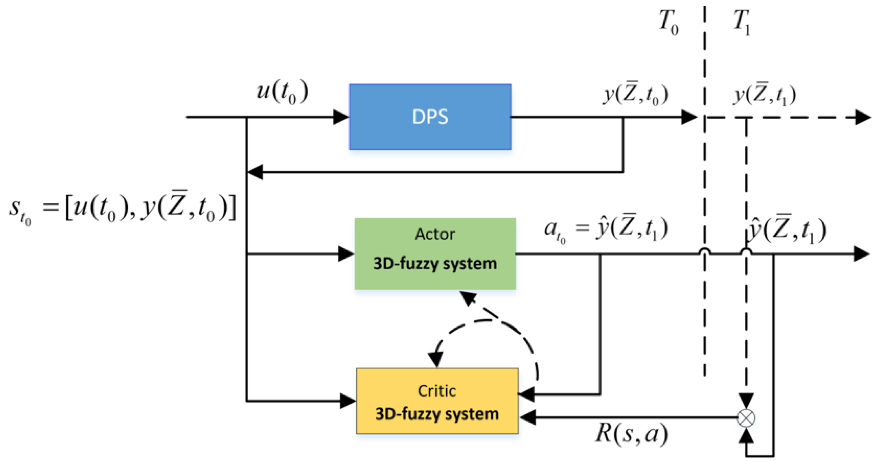
Figure 3 illustrates the architecture of the suggested online modeling method, where two 3D fuzzy systems are used. One is taken as the function of actor and the other is viewed as the role of a critic. The actor 3D fuzzy system serves as the DPS model, which takes $s_t$ as input and exports the predicted value $\widehat{y}(\overline{Z},t+1)$ as action at every time step t, then the environment exports reward R according to Equation (7). The critic-3D fuzzy system takes the state $s_t$ and the action $a_t$ as input and exports the action value $Q(s_t,a_t)$. The main process of the proposed algorithm is interleaving evaluation and improvement of the actor’s policy. This work employs the temporal-difference method to assess the action value function $Q(s,a)$ (also known as the critic function) and thereafter enhance the actor’s policy by adjusting the policy along the gradient of the function.

3.2. 3D Fuzzy Deterministic Policy Gradient Reinforcement Learning for DPS Online Modeling

Given the MDP model of the DPS modeling problem, the fusion of reinforcement learning and the 3D fuzzy system produces a novel 3D fuzzy reinforcement learning algorithm for DPS online modeling.

In order to describe the 3D fuzzy reinforcement learning algorithm well, we first introduce the principle of the deterministic policy gradient algorithm and 3D fuzzy modeling.

3.2.1. Deterministic Policy Gradient Algorithm

Deterministic policy gradient (DPG) is a specific type of policy gradient method that aims to optimize $J\left(\theta \right)$. The fundamental concept underlying the DPG is to modify the policy parameters $\theta$ in accordance with the gradient ${\nabla }_{\theta }J\left({\mu }_{\theta }\right)$ of the performance measure. The DPG typically relies on the actor–critic architecture, as depicted in Figure 4.

The deterministic policy gradient theorem examines a policy function ${\mu }_{\theta }\left(s\right)=\mu \left(s\right|\theta )$ that is deterministic and has a parameter vector $\theta$ for the policy. The term ’deterministic’ indicates that the action is chosen based on a deterministic policy ${\mu }_{\theta }:S->A$ with parameter $\theta \in R^n$, rather than a policy represented by a parametric probability distribution, which is known as SPG. The existence of the DPG is demonstrated in Reference [45] and the DPG theorem is established.

Assuming that the MDP fulfills the conditions ${\mu }_{\theta }\left(s\right)$, ${\nabla }_{\theta }{\mu }_{\theta }\left(s\right)$, $r(s,a)$ and ${\nabla }_{a}r(s,a)$, which are continuous in all parameters and variables $s,a,s^{\prime }$, it can be inferred that the conditions ${\nabla }_{\theta }u\left(s\right|\theta )$ and ${\nabla }_a{Q}^u(s,a)$ also exist and consequently, the DPG exists. Then:

$${\nabla }_{\theta }J\left({\mu }_{\theta }\right)=E_{s\sim {\rho }^{\mu }}\left[{\nabla }_{\theta }{\mu }_{\theta }\left(s\right){\nabla }_a{Q}^{\mu }(s,a){|}_{a={\mu }_{\theta }\left(s\right)}\right]$$

(8)

where $Q^{\mu }(s,a)$ represents the action value function, ${\rho }^{\mu }\left(s\right)$ represents the discounted state distribution (analogous to the stochastic case) and $J\left({\mu }_{\theta }\right)$ represents the performance objective. These variables are defined with regard to a deterministic policy $\mu$ and parameter $\theta$. Empirical evidence shows that the DPG algorithm can achieve superior performance compared to stochastic algorithms when dealing with high-dimensional action spaces [45]. Additionally, DPG is able to circumvent the challenges associated with integrating throughout the entire action space.

3.2.2. 3D Fuzzy Modeling

3D fuzzy modeling [21] is an innovative intelligent modeling method designed for nonlinear DPSs in recent years. This method presents a novel fuzzy model equipped to handle and articulate time/space-coupled information. The 3D fuzzy model is distinct from conventional fuzzy models as it is based on the concept of 3D fuzzy sets [21].

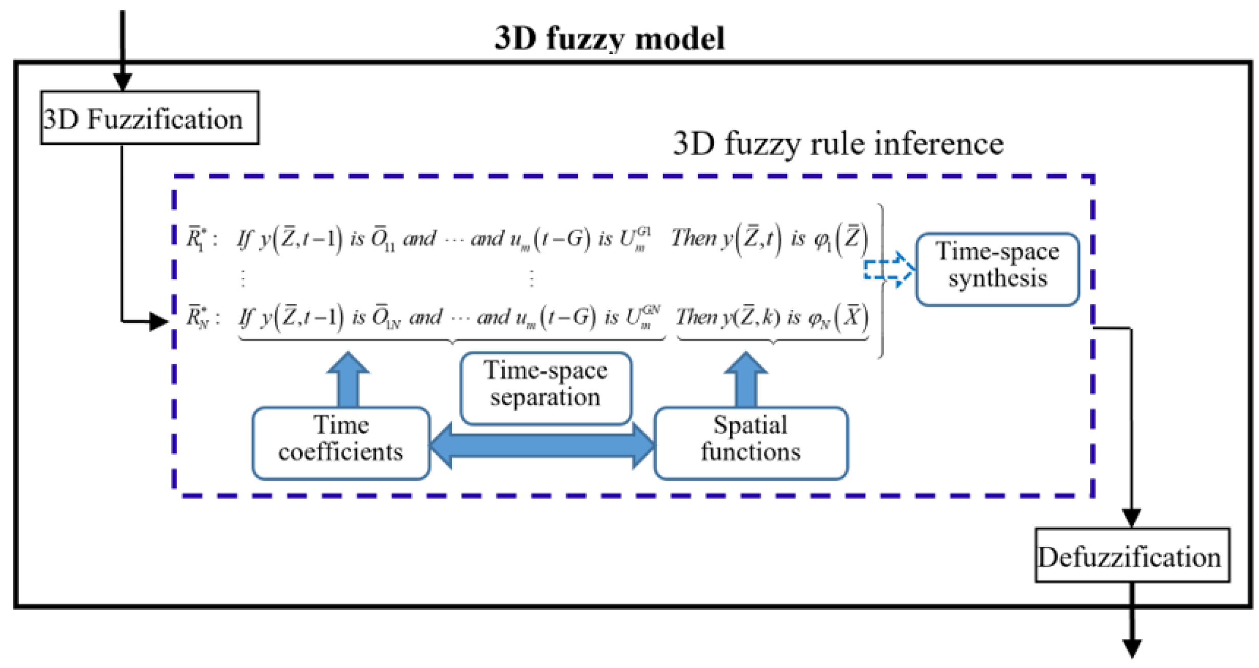
As demonstrated in Figure 5, the 3D fuzzy model provides a cohesive structure for effectively combining time–space separation with time–space reconstruction. Therefore, it can be inferred that DPS modeling is achievable regardless of the necessity of model reduction within the context of the 3D fuzzy model.

The 3D fuzzy rule in Figure 5 is rewritten as in Equation (9).

$$\left\{\begin{array}{cc}\hfill & {\overline{R}}_1^{*}:Ify\left(\overline{Z},t-1\right)is{\overline{O}}_{11}and\cdots and{u}_m\left(t-G\right)is{U}_m^{G1}Theny\left(\overline{Z},t\right)is{\phi }_1\left(\overline{Z}\right)\hfill \\ \hfill & ⋮⋮\hfill \\ \hfill & {\overline{R}}_N^{*}:Ify\left(\overline{Z},t-1\right)is{\overline{O}}_{1N}and\cdots and{u}_m\left(t-G\right)is{U}_m^{GN}Theny\left(\overline{Z},t\right)is{\phi }_N\left(\overline{Z}\right)\hfill \end{array}\right.$$

(9)

where ${\phi }_l\left(\overline{Z}\right)$ denotes a space base function, ${\overline{O}}_{sl}$ denotes a 3D fuzzy set, $U_g^{hl}$ denotes a conventional fuzzy set, $h=1,2,...,G,g=1,2,...,m,s=1,2,...,K,l=1,2,...,N$, N indicates the quantity of fuzzy rules.

The preceding component in ${\overline{R}}_l^{*}$ is utilized to calculate temporal coefficients, while the resulting component in ${\overline{R}}_l^{*}$ is utilized to depict space functions. The rule ${\overline{R}}_l^{*}$ intrinsically accomplishes the role of separating time and space, similar to the traditional modeling of time and space in DPS. The process of time–space reconstruction is achieved by combining active 3D fuzzy rules. It has been shown that the 3D fuzzy model has the ability to approximate any function universally [46].

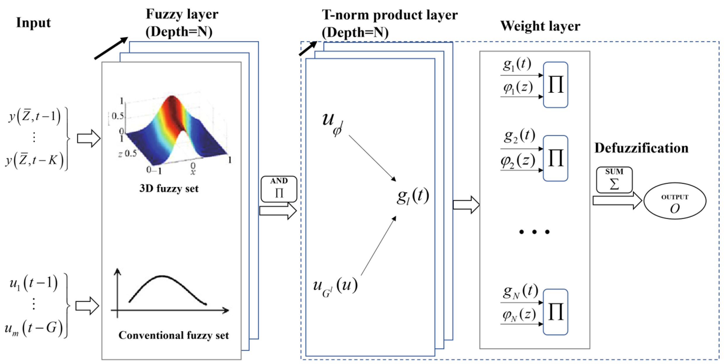
Like the neural network, the 3D fuzzy model also has the layer structure shown in Figure 6.

The 3D fuzzy model is presumed to possess two distinct categories of inputs. One is the measured space–time coupled data $[y(\overline{Z},t-1),y(\overline{Z},t-2),...,y(\overline{Z},t-K)]$ with $y(\overline{Z},t)=[y(f_1,t),\cdots ,y(f_p,t)]$; the other is traditional data $u=[u_1(t-1),\dots ,u_m(t-G)]$. Within the fuzzy layer, there exist conventional fuzzy sets and 3D fuzzy sets that correspond to two distinct types of inputs. Suppose a Gaussian-type membership function is used. The “and” operation of multiple 3D fuzzy memberships and the “and” operation of multiple conventional memberships of the inputs are shown as Equations (10) and (11).

$${\mu }_{{\phi }^l}=\sum _{j=1}^p{a}_j\prod _{i=1}^{K}exp(-{((y(f_j,t-i)-c_{ij}^l)/{\sigma }_{ij}^l)}^2)$$

(10)

$${\mu }_{G^l}=\prod _{i=1}^m\prod _{k=1}^{G}exp(-{((u_i(t-k)-d_{ik}^l)/{\delta }_{ik}^l)}^2)$$

(11)

where $c_{ij}^l$ and ${\sigma }_{ij}^l$ denote the centroid and spread of the Gaussian 3D fuzzy set ${\overline{O}}_{il}$ at the jth sensor position; $d_{ik}^l$ and ${\delta }_{ik}^l$ represent the centroid and spread of the conventional Gaussian fuzzy set $U_i^{kl}$; $a_j$ represents the weight of the $jth$ sensor position.

In the t-norm product layer, the active intensity of the rule is determined via combining the membership of each input in each rule, as in Equation (12).

$$g_l\left(t\right)={\mu }_{{\phi }^l}{\mu }_{G^l}$$

(12)

In the weight layer, the active rules are normalized and output is given as Equation (13).

$$O={\displaystyle \frac{{\displaystyle \sum _{i=1}^N}{g}_l\left(t\right){\phi }_l\left(\overline{Z}\right)}{{\displaystyle \sum _{i=1}^N}{g}_l\left(t\right)}}$$

(13)

where O represents the output generated by the 3D fuzzy model. Weight layer is known as the weight average defuzzification method. Up to now, 3D fuzzy modeling belongs to the offline category. In the next subsection, we will introduce the online 3D fuzzy modeling method based on reinforcement learning in detail.

3.2.3. 3DFDPG Modeling Method

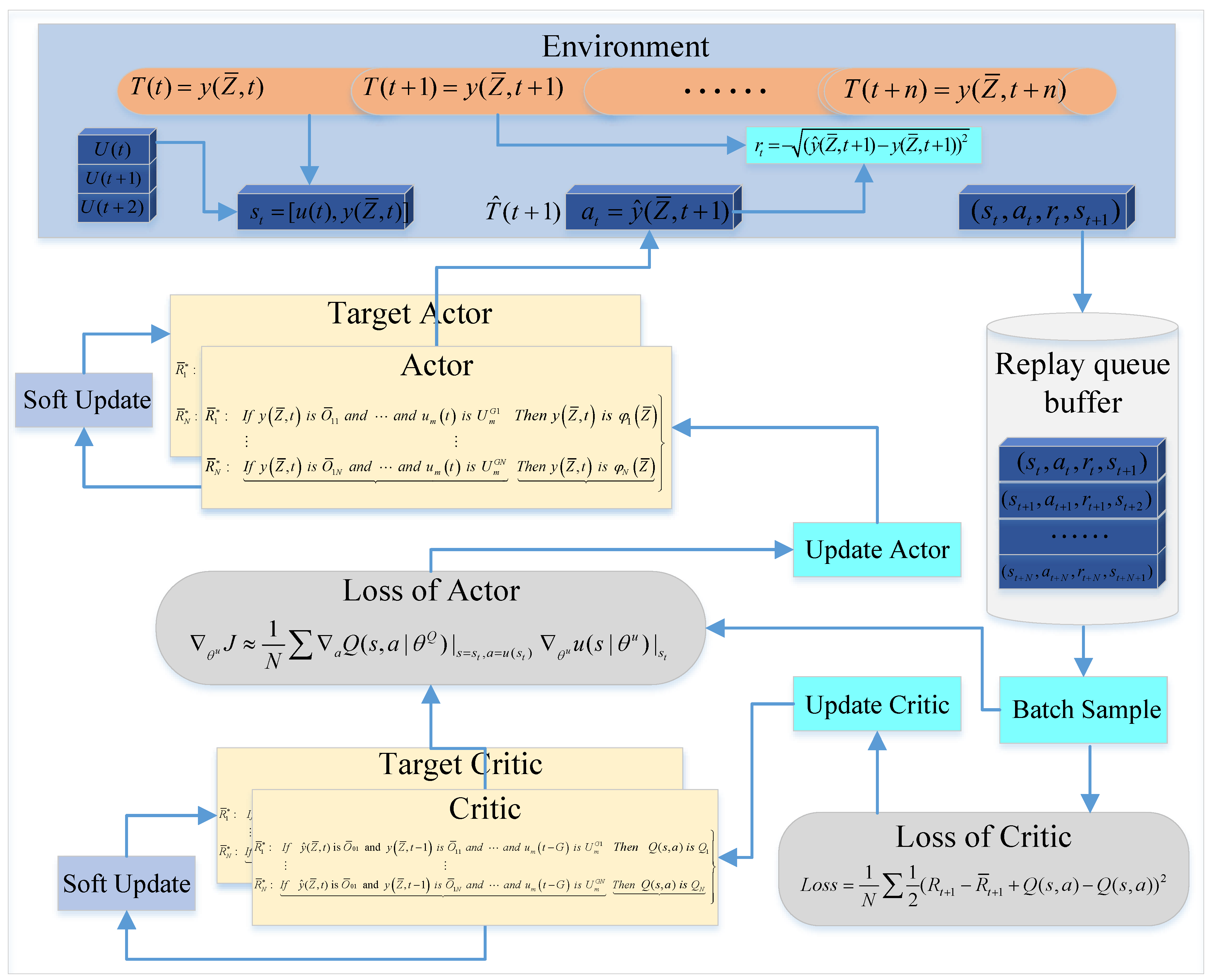
The fusion of deterministic policy gradient algorithm and 3D fuzzy system generates 3D fuzzy deterministic policy gradient reinforcement (3DFDPG) learning. When it is used as DPS online modeling, we call it 3DFDPG modeling for short. Figure 7 illustrates the detailed structural framework of 3DFDPG modeling.

As seen in Figure 7, the environment is composed by a DPS. $T\left(t\right)$ is the DPS’s output at time step t, i.e., $T\left(t\right)=y(\overline{Z},t)$. $u\left(t\right)$ is the DPS’s input. The state $s_t$, action $a_t$, reward $r_t$ and next state $s_{t+1}$ of the environment are set as $s_t=(u\left(t\right),y(\overline{Z},t))$, $a_t=\widehat{y}(\overline{Z},t+1)$, $r_t=-\sqrt{{(\widehat{y}(\overline{Z},t+1)-y(\overline{Z},t+1))}^2}$ and $s_{t+1}=(u(t+1),y(\overline{Z},t+1))$, respectively. The 3DFDPG algorithm utilizes an actor–critic structure as its foundation. The actor receives an environmental state as input and generates an action to be applied to the environment. The environment provides a subsequent state and a reward based on the action taken. The critic receives the actor’s action and the current state of the environment as input and produces an action value (also known as Q-value) for the specific state–action combination. The critic’s parameters are updated using the TD error. On the other hand, the actor’s parameters are updated by moving in the direction of the gradient of the action value function. Reinforcement learning may be prone to instability or be divergent when the action value function is represented by a nonlinear function approximator. To address this issue, the use of a replay buffer and target value method [38] is recommended.

Online DPS modeling is a continuous problem where the ongoing interaction between the actor and the environment is perpetual, lacking any termination states; therefore, the average reward setting [47] is needed. The average reward rate is defined as Equation (14).

$$\begin{array}{cc}\hfill R\left(\mu \right)& =\underset{h\to \infty }{lim}{\displaystyle \frac{1}{h}}\sum _{t=1}^h\mathbb{E}\left[R_t\right|S_0,A_{0:t-1\sim \pi }]\hfill \\ \hfill & =\underset{t\to \infty }{lim}\mathbb{E}\left[R_t\right|S_0,A_{0:t-1\sim \pi }]\hfill \\ \hfill & =\sum _{s\in S}\tau \left(s\right)\sum _{a\in A}\mu \left(a\right|s)\sum _{s^{\prime }\in S,r}p(s^{\prime },r|s,a)r\hfill \end{array}$$

(14)

where $\tau$ represents a stable distribution given the condition of $\mu$, S is a set of states, A is a set of actions, $p:S\times A\times S\times R\to [0,1]$ is the state transition probability which implies the dynamics of the environment and r is the reward at every time step. In the average reward setting, returns are defined in terms of differences between rewards and the average reward, as in Equation (15).

$$G_t\doteq R_{t+1}-R\left(\mu \right)+R_{t+2}-R\left(\mu \right)+R_{t+3}-R\left(\mu \right)+\cdots$$

(15)

where $G_t$ is the long time return, $R_{t+1}$ is the reward at time step $t+1$ and $R\left(\mu \right)$ is the average reward under the policy $\mu$.

Then, the action value functions $Q(s,a)$ for all $s\in S,a\in A$ are defined as in Equation (16).

$$\begin{array}{cc}\hfill Q(s,a)& ={\mathbb{E}}_{\mu }\left[G_t\right|S_t=s,A_t=a]\hfill \\ \hfill & =\mathbb{E}[R_{t+1}-R\left(\mu \right)+G_{t+1}|S_t=s,A_t=a]\hfill \\ \hfill & =\mathbb{E}[R_{t+1}-R\left(\mu \right)+Q(S_{t+1},A_{t+1})|S_t=s,A_t=a]\hfill \\ \hfill & =\sum _a\mu \left(a\right|s)\sum _{s^{\prime },r}p(s^{\prime },r|s,a)[r-R\left(\mu \right)+v\left(s^{\prime }\right)]\hfill \end{array}$$

(16)

The Bellman equation of the action value function $Q(s,a)$ for all $a\in A,s\in S$ is defined as Equation (17).

$$\begin{array}{cc}\hfill Q(s,a)& =\mathbb{E}[R_{t+1}-R\left(\mu \right)+Q(S_{t+1},A_{t+1})|S_t=s,A_t=a]\hfill \end{array}$$

(17)

Then, the TD error is defined as Equation (18).

$${\delta }_t\doteq R_{t+1}-{\overline{R}}_{t+1}+\widehat{Q}(S_{t+1},A_{t+1})-\widehat{Q}(S_t,A_t)$$

(18)

where ${\overline{R}}_{t+1}$ is an estimate at time $t+1$ of the average reward $R\left(\mu \right)$ and $\widehat{Q}(S_t,A_t)$ is an estimate at time t of the action value function.

The average reward is updated by a soft style as in Equation (19).

$${\overline{R}}_{t+1}=\beta {\overline{R}}_t+(1-\beta ){\delta }_t$$

(19)

where $\beta$ represents the update factor.

The mathematical description of the actor and critic is shown below. The actor function $\mu \left(s\right)$’s structure is constructed as in Equation (9), which is rewritten as Equation (20)

$$\left\{\begin{array}{cc}\hfill & {\overline{R}}_1^{*}:Ify\left(\overline{Z},t-1\right)is{\overline{O}}_{11}and\cdots and{u}_m\left(t-G\right)is{U}_m^{G1}Theny\left(\overline{Z},t\right)is{\phi }_1\left(\overline{Z}\right)\hfill \\ \hfill & ⋮⋮\hfill \\ \hfill & {\overline{R}}_N^{*}:Ify\left(\overline{Z},t-1\right)is{\overline{O}}_{1N}and\cdots and{u}_m\left(t-G\right)is{U}_m^{GN}Theny\left(\overline{Z},t\right)is{\phi }_N\left(\overline{Z}\right)\hfill \end{array}\right.$$

(20)

If the Gaussian-type member function, singleton 3D fuzzification, average defuzzification and product t-norm are selected for a 3D fuzzy model, the following nonlinear mathematical statement is provided as Equation (21).

$$\begin{array}{cc}\hfill \mu \left(s\right)& =\widehat{y}(\overline{Z},t)\hfill \\ \hfill & ={\displaystyle \frac{{\sum }_{i=1}^N\left\{\begin{array}{c}{\sum }_{j=1}^p{a}_j^l{\prod }_{i=1}^{K}exp(-{((y(f_j,t-i)-c_{ij}^l)/{\sigma }_{ij}^l)}^2)\\ \times {\prod }_{i=1}^m{\prod }_{k=1}^{G}exp(-{((u_i(t-k)-d_{ik}^l)/{\delta }_{ik}^l)}^2)\end{array}\right\}{\phi }_l\left(\overline{Z}\right)}{{\sum }_{i=1}^N\left\{\begin{array}{c}{\sum }_{j=1}^P{a}_j^l{\prod }_{i=1}^{J}exp(-{((y(f_j,t-i)-c_{ij}^l)/{\sigma }_{ij}^l)}^2)\\ \times {\prod }_{i=1}^m{\prod }_{k=1}^{G}exp(-{((u_i(t-k)-d_{ik}^l)/{\delta }_{ik}^l)}^2)\end{array}\right\}}}\hfill \\ \hfill & ={\displaystyle \frac{{\sum }_{i=1}^N{g}_l\left(t\right){\phi }_l\left(\overline{Z}\right)}{{\sum }_{i=1}^N{g}_l\left(t\right)}}\hfill \end{array}$$

(21)

where

$g_l\left(t\right)={\mu }_{{\phi }^l}\ast {\mu }_{G^l}$,

${\mu }_{{\phi }^l}={\displaystyle \sum _{j=1}^p}{a}_j{\displaystyle \prod _{i=1}^K}exp(-{((y(f_j,t-i)-c_{ij}^l)/{\sigma }_{ij}^l)}^2)$,

${\mu }_{G^l}={\displaystyle \prod _{i=1}^m}{\displaystyle \prod _{k=1}^G}exp(-{((u_i(t-k)-d_{ik}^l)/{\delta }_{ik}^l)}^2)$.

${\phi }_l\left(\overline{Z}\right)$ is the Fourier base function, which can be given as Equation (22).

$${\phi }_l\left(\overline{Z}\right)=a_{l}sin\left(b_l\overline{Z}\right)+c_{l}cos\left(b_l\overline{Z}\right)+d_l$$

(22)

The action value function $Q(s,a)$ is constructed with the structure as expressed in Equation (23).

$$\left\{\begin{array}{cc}\hfill & {\overline{R}}_1^{*}:If\widehat{y}(\overline{Z},t)\mathrm{is}{\overline{O}}_{01}\mathrm{and}y\left(\overline{Z},t-1\right)is{\overline{O}}_{11}and\cdots and{u}_m\left(t-G\right)is{U}_m^{G1}\hfill \\ & ThenQ(s,a)is{Q}_1\hfill \\ \hfill & ⋮⋮\hfill \\ \hfill & {\overline{R}}_N^{*}:If\widehat{y}(\overline{Z},t)\mathrm{is}{\overline{O}}_{0N}\mathrm{and}y\left(\overline{Z},t-1\right)is{\overline{O}}_{1N}and\cdots and{u}_m\left(t-G\right)is{U}_m^{GN}\hfill \\ \hfill & ThenQ(s,a)is{Q}_N\hfill \end{array}\right.$$

(23)

where $U_g^{hl}$ represents a conventional fuzzy set, ${\overline{O}}_{sl}$ represents a 3D fuzzy set, $Q_l$ represents a constant, $g=1,2,...,m,s=0,1,...,K,l=1,2,...,N,h=1,2,...,G$ and N indicates the quantity of fuzzy rules.

Similar to the actor function, Equation (24) is provided for the mathematical expression of the action value function $Q(s,a)$.

$$\begin{array}{cc}\hfill Q(s,a)& =\begin{array}{cc}\hfill & {\displaystyle \frac{{\displaystyle \sum _{l=1}^N}\left\{\begin{array}{cc}\hfill & {\displaystyle \sum _{j=1}^P}{a}_j^{l}exp(-{((\widehat{y}(f_j,t)-c_{0j}^l)/{\sigma }_{0j}^l)}^2){\displaystyle \sum _{j=1}^P}{a}_j^l{\displaystyle \prod _{i=1}^K}exp(-{((y(f_j,t-i)-c_{ij}^l)/{\sigma }_{ij}^l)}^2)\hfill \\ \hfill & \times {\displaystyle \prod _{\mathrm{i}=1}^m}{\displaystyle \prod _{k=1}^G}exp(-{((u_i(t-k)-d_i^{kl})/{\delta }_i^{kl})}^2)\hfill \end{array}\right\}}{{\displaystyle \sum _{l=1}^N}\left\{\begin{array}{cc}\hfill & {\displaystyle \sum _{j=1}^P}{a}_j^{l}exp(-{((\widehat{y}(f_j,t)-c_{0j}^l)/{\sigma }_{0j}^l)}^2){\displaystyle \sum _{j=1}^P}{a}_j^l{\displaystyle \prod _{i=1}^K}exp(-{((y(f_j,t-i)-c_{ij}^l)/{\sigma }_{ij}^l)}^2)\hfill \\ \hfill & \times {\displaystyle \prod _{\mathrm{i}=1}^m}{\displaystyle \prod _{k=1}^K}exp(-{((u_i(t-k)-d_i^{kl})/{\delta }_i^{kl})}^2)\hfill \end{array}\right\}}}\hfill \\ \hfill & \hfill \end{array}{Q}_l\hfill \\ \hfill & ={\displaystyle \frac{{\sum }_{i=1}^N{h}_l\left(t\right)Q_l}{{\sum }_{i=1}^N{h}_l\left(t\right)}}\hfill \end{array}$$

(24)

where

$h_l\left(t\right)={\mu }_{d^l}{\mu }_{{\phi }^l}{\mu }_{G^l}$,

${\mu }_{d^l}=exp(-{((\widehat{y}(f_i,t)-c_{0j}^l)/{\sigma }_{0j}^l)}^2)$,

${\mu }_{{\phi }^l}={\displaystyle \sum _{j=1}^p}{a}_j{\displaystyle \prod _{i=1}^K}exp(-{((y(f_j,t-i)-c_{ij}^l)/{\sigma }_{ij}^l)}^2)$,

${\mu }_{G^l}={\displaystyle \prod _{i=1}^m}{\displaystyle \prod _{k=1}^G}exp(-{((u_i(t-k)-d_{ik}^l)/{\delta }_{ik}^l)}^2)$.

3.3. Update Process of Parameters for 3D Fuzzy Systems

For a discrete state–action space with restricted options, the action value of each state may be enumerated, that is, tabular reinforcement learning. In the tabular reinforcement learning, the action value $Q(s,a)$ is updated by the Bellman equation [47]. Then, the policy optimization is completed by taking the maximum action a corresponding to different states. As the action value function $Q(s,a)$ is a continuous function, it is challenging to determine the utmost value when the state action space is continuous. Instead, a straightforward and computationally appealing alternative is to shift the policy in the direction of the gradient of $Q(s,a)$, rather than globally maximizing $Q(s,a)$.

The action value function is specified by the following Equation (25):

$$Q(s,a)=\mathbb{E}\left[G_t\right|S_t=s,A_t=a]$$

(25)

Equation (25) shows that $Q(s,a)$ is the expected return after taking action a and following strategy $\mu$ from state s. The goal of reinforcement learning is to find an optimal strategy to maximize $Q(s,a)$ for each state action pair, which is equivalent to maximizing the total expected return $G_t$. Equation (26) gives the return $G_t$ as the sum of future rewards:

$$G_t=R_{t+1}-R\left(\mu \right)+R_{t+2}-R\left(\mu \right)+R_{t+3}-R\left(\mu \right)+\cdots +R_{t+N}-R\left(\mu \right)$$

(26)

where $R_{t+1}$, $R_{t+2}$, $R_{t+3}$, ⋯ is the immediate reward for the future time step and $R\left(\mu \right)$ is the average reward under strategy $\mu$. Since $R\left(\mu \right)$ remains unchanged under the same strategy $\mu$, in order to maximize $G_t$, it is necessary to maximize every reward $R_{t+1},R_{t+2},\cdots ,R_{t+N}$ in the future. According to Equation (7), it is established that when the immediate reward $R_t$ reaches its maximum value, the discrepancy between the predicted output of the online 3DFDPG model and the actual system output is zero. If the immediate reward $R_t$ is not at its peak value, then a bigger $R_t$ results in increased model accuracy, but a lower $R_t$ leads to decreased accuracy. Therefore, the 3DFDPG algorithm maximizes the action value function $Q(s,a)$ by updating the strategy $\mu$, which is equivalent to maximizing the expected return $G_t$ by maximizing the immediate reward.

So the performance objective $J\left({\mu }_{\theta }\right)$ is defined as in Equation (27).

$$J\left({\mu }_{\theta }\right)=E_{s\sim {\mu }_{\theta }}\left[Q(s,a)\right]$$

(27)

By the chain rule, the update of policy’s parameters is shown as Equation (28).

$${\theta }_{k+1}^{\mu }={\theta }_k^{\mu }+\alpha {\displaystyle \frac{1}{N}}\sum {\nabla }_{a}Q(s,a|{\theta }^Q){|}_{s=s_t,a=\mu \left(s_t\right)}{\nabla }_{{\theta }_k^{\mu }}\mu \left(s\right|{\theta }^{\mu }){|}_{s_t}$$

(28)

where ${\theta }_k^{\mu }$ is the parameters of the policy $\mu$, N is the number of samples and $\alpha$ is the learning rate.

The critic function takes TD(0) as the target; the loss function is shown as Equation (29).

$$Loss={\displaystyle \frac{1}{N}}\sum {\displaystyle \frac{1}{2}}{(y_t-Q(s,a)|{\theta }^Q)}^2$$

(29)

where $y_t$ is the $TD\left(0\right)$ target defined as Equation (30).

$$y_t=r_t-{\overline{R}}_t+Q^{\prime }(s_{t+1},{\mu }^{\prime }\left(s_{t+1}\right|{\theta }^{u^{\prime }})|{\theta }^{Q^{\prime }})$$

(30)

The update of the action value function’s parameters is shown as Equation (31).

$${\theta }_{k+1}^Q={\theta }_k^Q+\alpha {\displaystyle \frac{1}{N}}\sum (y_t-Q(s,a)|{\theta }^Q){\nabla }_{{\theta }^Q}Q(s,a|{\theta }^Q)$$

(31)

where ${\theta }_k^Q$ is the parameters of the action value function; the detail of the parameter’s updating is given in the following subsection.

In this paper, because of the instability that directly uses the 3D fuzzy system as the nonlinear approximators, the target critic and the target actor are adopted. Rather than updating the target parameters by directly copying the original 3D fuzzy model’s parameters, Equation (32) is utilized to modify the parameters of the target 3D fuzzy model.

$$\begin{array}{c}\hfill {\theta }^{Q^{\prime }}=\gamma {\theta }^Q+(1-\gamma ){\theta }^{Q^{\prime }}\\ \hfill {\theta }^{{\mu }^{\prime }}=\delta {\theta }^{\mu }+(1-\delta ){\theta }^{{\mu }^{\prime }}\end{array}$$

(32)

where $\gamma$ and $\delta$ are the update factors.

3.3.1. The Parameter Updating of the Actor Function in Detail

The actor described in Section 3.2.3 is updated by the performance objective as Equation (27). Equation (27) is subjected to the chain rule, resulting in the derivation of Equation (33).

$${\nabla }_{\theta }J\left({\mu }_{\theta }\right)=E\left[{\nabla }_{a}Q(s,a){|}_{a=\mu \left(s\right)}{\nabla }_{\theta }\mu \left(s\right)\right]$$

(33)

where $a=(\widehat{y}(f_1,t),\widehat{y}(f_2,t),\cdots ,\widehat{y}(f_p,t))$. Then, the partial derivative with respect to a yields Equation (34).

$${\nabla }_{a}Q(s,a)=({\nabla }_{\widehat{y}(f_1,t)}Q(s,a),{\nabla }_{\widehat{y}(f_2,t)}Q(s,a),\dots ,{\nabla }_{\widehat{y}(f_p,t)}Q(s,a))$$

(34)

$${\nabla }_{\widehat{y}(f_j,t)}Q(s,a)=\sum _{l=1}^N{\displaystyle \frac{𝜕Q}{𝜕h_l\left(t\right)}}{\displaystyle \frac{𝜕h_l\left(t\right)}{\widehat{y}(f_j,t)}}$$

(35)

From Equation (24), the term $𝜕Q/𝜕h_l\left(t\right)$ and the term $𝜕h_l\left(t\right)/\widehat{y}(f_j,t)$ can be determined by Equations (36) and (37).

$${\displaystyle \frac{𝜕Q}{𝜕h_l\left(t\right)}}={\displaystyle \frac{Q_l-Q}{{\sum }_{i=1}^N{h}_l\left(t\right)}}$$

(36)

$${\displaystyle \frac{𝜕h_l\left(t\right)}{\widehat{y}(f_j,t)}}={\mu }_{{\phi }^l}{\mu }_{G^l}{a}_{j}exp(-{((\widehat{y}(f_j,t)-c_{0j}^l)/{\sigma }_{0j}^l)}^2){\displaystyle \frac{-2(\widehat{y}(f_j,t)-c_{0j}^l)}{{\left({\sigma }_{0j}^l\right)}^2}}$$

(37)

Substituting Equations (36) and (37) into (35), the gradient of Q in relation to a is given as in Equation (38).

$${\nabla }_{\widehat{y}(z_j,t)}Q(s,a)=\sum _{l=1}^N{\displaystyle \frac{Q_l-Q}{{\sum }_{i=1}^N{h}_l\left(t\right)}}{\mu }_{{\phi }^l}{u}_{G^l}{a}_{j}exp(-{((\widehat{y}(z_j,t)-c_{0j}^l)/{\sigma }_{0j}^l)}^2){\displaystyle \frac{-2(\widehat{y}(z_j,t)-c_{0j}^l)}{{\left({\sigma }_{0j}^l\right)}^2}}$$

(38)

According to the same process as above, we can obtain $𝜕\mu \left(s\right)/𝜕{\theta }^u$. ${\theta }^{\mu }$ is the parameter vector of the actor function, described by Equation (39).

$${\theta }^{\mu }=(c_{ij}^l,{\sigma }_{ij}^l,d_{ik}^l,{\delta }_{ik}^l,a_l,b_l,c_l,d_l)(j=1,\dots ,p;i=1,\dots ,m;l=1,\dots ,N)$$

(39)

Then, the partial derivative of the policy with respect to the parameter $\theta$ is shown in Equation (40).

$${\nabla }_{\theta }\mu \left(s\right)=({\displaystyle \frac{𝜕\mu }{c_{ij}^l}},{\displaystyle \frac{𝜕\mu }{{\sigma }_{ij}^l}},{\displaystyle \frac{𝜕\mu }{d_{ik}^l}},{\displaystyle \frac{𝜕\mu }{{\delta }_{ik}^l}},{\displaystyle \frac{𝜕\mu }{a_l}},{\displaystyle \frac{𝜕\mu }{b_l}},{\displaystyle \frac{𝜕\mu }{c_l}},{\displaystyle \frac{𝜕\mu }{d_l}})$$

(40)

where $c_{ij}^l$ and ${\sigma }_{ij}^l$ denote the centroid and spread of the Gaussian 3D fuzzy set ${\overline{O}}_{il}$ at the $jth$ sensor position; $d_{ik}^l$ and ${\delta }_{ik}^l$ represent the centroid and spread of the conventional Gaussian fuzzy set $U_i^{kl}$, $a_l,b_l,c_l,d_l$ denote the coefficients of the base function in Fourier space.

From Equations (21) and (22), we can derive the partial derivative of the policy ${\displaystyle \frac{𝜕\mu }{c_{ij}^l}}$, ${\displaystyle \frac{𝜕\mu }{{\sigma }_{ij}^l}}$, ${\displaystyle \frac{𝜕\mu }{d_{ik}^l}}$, ${\displaystyle \frac{𝜕\mu }{{\delta }_{ik}^l}}$, ${\displaystyle \frac{𝜕\mu }{a_l}}$, ${\displaystyle \frac{𝜕\mu }{b_l}}$, ${\displaystyle \frac{𝜕\mu }{c_l}}$, ${\displaystyle \frac{𝜕\mu }{d_l}}$, shown as Equations (41)–(48).

$${\displaystyle \frac{𝜕\mu }{c_{ij}^l}}={\displaystyle \frac{{\phi }_l\left(\overline{Z}\right)-\mu \left(s\right)}{{\displaystyle \sum _{i=1}^N}{g}_l\left(t\right)}}{u}_{G^l}{a}_{j}exp(-{((y(f_j,t-1)-c_{ij}^l)/{\sigma }_{ij}^l)}^2){\displaystyle \frac{2(y(f_j,t-1)-c_{ij}^l)}{{\left({\sigma }_{ij}^l\right)}^2}}$$

(41)

$${\displaystyle \frac{𝜕\mu }{{\sigma }_{ij}^l}}={\displaystyle \frac{{\phi }_l\left(\overline{Z}\right)-\mu \left(s\right)}{{\displaystyle \sum _{i=1}^N}{g}_l\left(t\right)}}{\mu }_{G^l}{a}_j\prod _{i=1}^{K}exp(-{((y(f_j,t-i)-c_{ij}^l)/{\sigma }_{ij}^l)}^2){\displaystyle \frac{2{(y(f_j,t-i)-c_{ij}^l)}^2}{{\left({\sigma }_{ij}^l\right)}^3}}$$

(42)

$${\displaystyle \frac{𝜕\mu }{d_{ik}^l}}={\displaystyle \frac{{\phi }_l\left(\overline{Z}\right)-\mu \left(s\right)}{{\displaystyle \sum _{i=1}^N}{g}_l\left(t\right)}}{\mu }_{{\phi }^l}\prod _{i=1}^m\prod _{k=1}^{G}exp(-{((u_i(t-k)-d_{ik}^l)/{\delta }_{ik}^l)}^2){\displaystyle \frac{2(u_i(t-k)-{\delta }_{ik}^l)}{{\left({\delta }_{ik}^l\right)}^2}}$$

(43)

$${\displaystyle \frac{𝜕\mu }{{\delta }_{ik}^l}}={\displaystyle \frac{{\phi }_l\left(\overline{Z}\right)-\mu \left(s\right)}{{\displaystyle \sum _{l=1}^N}{g}_l\left(t\right)}}{u}_{{\phi }^l}\prod _{i=1}^{m}exp(-{((u_i(t-1)-d_{ik}^l)/{\delta }_{ik}^l)}^2){\displaystyle \frac{2{(u_i(t-1)-d_{ik}^l)}^2}{{\left({\delta }_{ik}^l\right)}^3}}$$

(44)

$${\displaystyle \frac{𝜕\mu }{a_l}}={\displaystyle \frac{g_l\left(t\right)}{{\displaystyle \sum _{l=1}^N}{g}_l\left(t\right)}}sin\left(b_l\overline{Z}\right)$$

(45)

$${\displaystyle \frac{𝜕\mu }{b_l}}={\displaystyle \frac{g_l\left(t\right)}{{\displaystyle \sum _{l=1}^N}{g}_l\left(t\right)}}{a}_l\overline{Z}cos\left(b_l\overline{Z}\right)-c_l\overline{Z}sin\left(b_l\overline{Z}\right)$$

(46)

$${\displaystyle \frac{𝜕\mu }{c_l}}={\displaystyle \frac{g_l\left(t\right)}{{\displaystyle \sum _{l=1}^N}{g}_l\left(t\right)}}cos\left(b_l\overline{Z}\right)$$

(47)

$${\displaystyle \frac{𝜕\mu }{d_l}}={\displaystyle \frac{g_l\left(t\right)}{{\displaystyle \sum _{l=1}^N}{g}_l\left(t\right)}}$$

(48)

3.3.2. The Updating of the Parameters of the Critic Function in Detail

The critic function adopts the same structure as the actor function, as shown in Figure 6. Different to the actor function’s performance objective, the loss function of the critic function is as in Equation (18). To describe this clearly, here we write the equation again.

$${\theta }_{k+1}^Q={\theta }_k^Q+\alpha {\displaystyle \frac{1}{N}}\sum (y_t-Q(s,a)|{\theta }^Q){\nabla }_{{\theta }^Q}Q(s,a|{\theta }^Q)$$

(49)

where, ${\theta }^Q$ is the parameter vector of the critic function. N is the sample batch size. $\alpha$ is the learning rate. $y_t$ is the $TD\left(0\right)$ target defined as Equation (30), and ${\theta }^Q$ is defined as Equation (50).

$${\theta }^Q=(c_{0j}^l,{\sigma }_{0j}^l,c_{ij}^l,{\sigma }_{ij}^l,d_{ik}^l,{\delta }_{ik}^l,Q_l)(j=1,\dots ,p;i=1,\dots ,m;l=1,\dots ,N)$$

(50)

Then the partial derivative of $Q(s,a)$ with respect to ${\theta }^Q$ is shown in Equation (51); the detailed formulas are shown in Equations (52)–(58).

$${\nabla }_{{\theta }^Q}Q(s,a|{\theta }^Q)=({\displaystyle \frac{𝜕Q}{c_{0j}^l}},{\displaystyle \frac{𝜕Q}{{\sigma }_{0j}^l}},{\displaystyle \frac{𝜕Q}{c_{ij}^l}},{\displaystyle \frac{𝜕Q}{{\sigma }_{ij}^l}},{\displaystyle \frac{𝜕Q}{d_{ik}^l}},{\displaystyle \frac{𝜕Q}{{\delta }_{ik}^l}},{\displaystyle \frac{𝜕Q}{Q_l}})$$

(51)

$${\displaystyle \frac{𝜕Q}{c_{0j}^l}}={\displaystyle \frac{Q_l-Q}{{\displaystyle \sum _{i=1}^N}{h}_l\left(t\right)}}{\mu }_{G^l}{a}_{j}exp(-{((\widehat{y}(f_j,t)-c_{0j}^l)/{\sigma }_{0j}^l)}^2)\prod _{i=1}^{K}exp(-{((y(f_j,t-i)-c_{ij}^l)/{\sigma }_{ij}^l)}^2){\displaystyle \frac{2(\widehat{y}(z_j,t)-c_{0j}^l)}{{\left({\sigma }_{0j}^l\right)}^2}}$$

(52)

$${\displaystyle \frac{𝜕Q}{{\sigma }_{0j}^l}}={\displaystyle \frac{Q_l-Q}{{\displaystyle \sum _{i=1}^N}{h}_l\left(t\right)}}{\mu }_{G^l}{a}_{j}exp(-{((\widehat{y}(f_j,t)-c_{0j}^l)/{\sigma }_{0j}^l)}^2)\prod _{i=1}^{K}exp(-{((y(f_j,t-i)-c_{ij}^l)/{\sigma }_{ij}^l)}^2){\displaystyle \frac{2{(\widehat{y}(z_j,t)-c_{0j}^l)}^2}{{\left({\sigma }_{0j}^l\right)}^3}}$$

(53)

$${\displaystyle \frac{𝜕Q}{c_{ij}^l}}={\displaystyle \frac{Q_l-Q}{{\displaystyle \sum _{i=1}^N}{h}_l\left(t\right)}}{\mu }_{G^l}{a}_{j}exp(-{((\widehat{y}(f_j,t)-c_{0j}^l)/{\sigma }_{0j}^l)}^2)\prod _{i=1}^{K}exp(-{((y(f_j,t-i)-c_{ij}^l)/{\sigma }_{ij}^l)}^2){\displaystyle \frac{2(y(f_j,t)-c_{ij}^l)}{{\left({\sigma }_{ij}^l\right)}^2}}$$

(54)

$${\displaystyle \frac{𝜕Q}{{\sigma }_{ij}^l}}={\displaystyle \frac{Q_l-Q}{{\displaystyle \sum _{i=1}^N}{h}_l\left(t\right)}}{\mu }_{G^l}{a}_{j}exp(-{((\widehat{y}(f_j,t)-c_{0j}^l)/{\sigma }_{0j}^l)}^2)exp(-{((y(f_j,t-1)-c_{ij}^l)/{\sigma }_{ij}^l)}^2){\displaystyle \frac{2{(y(f_j,t)-c_{ij}^l)}^2}{{\left({\sigma }_{ij}^l\right)}^3}}$$

(55)

$${\displaystyle \frac{𝜕Q}{d_{ik}^l}}={\displaystyle \frac{Q_l-Q}{{\displaystyle \sum _{i=1}^N}{h}_l\left(t\right)}}{\mu }_{{\phi }^l}\prod _{i=1}^{m}exp(-{((u_i(t-1)-d_{ik}^l)/{\delta }_{ik}^l)}^2){\displaystyle \frac{2(u_i(t-1)-d_{ik}^l)}{{\left({\delta }_{ik}^l\right)}^2}}$$

(56)

$${\displaystyle \frac{𝜕Q}{{\delta }_{ik}^l}}={\displaystyle \frac{Q_l-Q}{{\displaystyle \sum _{i=1}^N}{h}_l\left(t\right)}}{\mu }_{{\phi }^l}\prod _{i=1}^{m}exp(-{((u_i(t-1)-d_{ik}^l)/{\delta }_{ik}^l)}^2){\displaystyle \frac{2{(u_i(t-1)-d_{ik}^l)}^2}{{\left({\delta }_{ik}^l\right)}^3}}$$

(57)

$${\displaystyle \frac{𝜕Q}{Q_l}}={\displaystyle \frac{h_l\left(t\right)}{{\sum }_{i=1}^N{h}_l\left(t\right)}}$$

(58)

3.3.3. The Process of the Proposed 3DFDPG

The proposed 3DFDPG is executed as follows.

Input: Batch size N, number of 3D fuzzy rules of policy $\mu \left(s\right)$ and action value function $Q(s,a)$, replay buffer size $N^{\prime }$, actor’s learning rate ${\alpha }_a$ and critic’s learning rate ${\alpha }_c$.

Step 1: Initialize critic $Q(s,a|{\theta }^Q)$ and policy $\mu \left(s\right|{\theta }^u)$ with parameters ${\theta }^Q=(c_{0j}^l,{\sigma }_{0j}^l,c_{ij}^l,{\sigma }_{ij}^l,d_{ik}^l,{\delta }_{ik}^l,Q_l)$ and ${\theta }^{\mu }=(c_{ij}^l,{\sigma }_{ij}^l,d_{ik}^l,{\delta }_{ik}^l,a_l,b_l,c_l,d_l)$ randomly.

Step 2: Initialize target ${\mu }^{\prime }$ and $Q^{\prime }$ with parameters ${\theta }^{{\mu }^{\prime }}={\theta }^{\mu }$ and ${\theta }^{Q^{\prime }}={\theta }^Q$. The average reward $\overline{R}=0$.

Step 3: Initialize replay buffer $RB$.

Step 4: Loop forever:

Step 5: Perform action $a_t$ on the DPS and analyze the resulting reward $r_t$ and subsequent state $s_{t+1}$ of the DPS.

Step 6: Preserve the transition $(s_t,a_t,r_t,s_{t+1})$ to $RB$.

Step 7: Randomly select a small quantity of $N^{\prime }$ transitions from $RB$.

Step 8: Set $y_i=r_i-\overline{R}+Q^{\prime }(s_{t+1},{\mu }^{\prime }\left(s_{t+1}\right|{\theta }^{{\mu }^{\prime }})|{\theta }^{Q^{\prime }})$.

Step 9: Set $\overline{R}=\beta \overline{R}+(1-\beta )\delta$.

Step 10: Minimize the loss function $Loss=1/N$∑$(y_t-Q(s,a)|{\theta }^Q{)}^2$ to update the critic.

Step 11: Utilize the policy gradient that was sampled to update the policy.

$${\nabla }_{{\theta }^{\mu }}J\approx {\displaystyle \frac{1}{N}}\sum {\nabla }_{a}Q(s,a|{\theta }^Q){|}_{s=s_t,a=\mu \left(s_t\right)}{\nabla }_{{\theta }^{\mu }}\mu \left(s\right|{\theta }^{\mu }){|}_{s_t}$$

Step 12: If the estimate error is less than a threshold $\delta$, update the policy parameters and directly use the error via stochastic gradient descent.

$$Error={\displaystyle \frac{1}{2}}{(y(\overline{Z},t)-\widehat{y}(\overline{Z},t))}^2$$

Step 13: Update the target ${\theta }^{Q^{\prime }}=\gamma {\theta }^Q+(1-\gamma ){\theta }^{Q^{\prime }},{\theta }^{{\mu }^{\prime }}=\delta {\theta }^{\mu }+(1-\delta ){\theta }^{{\mu }^{\prime }}$.

Step 14: Output the policy $\mu \left(s_t\right|{\theta }^{\mu })$ as the model of the DPS at every time step.

4. Applications

The typical distributed parameter system (RTCVD) depicted in Section 2 is considered to assess the efficacy of the suggested algorithm 3DFDPG. To obtain sufficient dynamic knowledge about the system, the system manipulates the input variable $u_1$, $u_2$ and $u_3$ to add the interference signal whose amplitude is not more than 10%. Therefore, three input variables with interference signals can be given in the following ways.

$$\begin{array}{c}\hfill u_1\left(t\right)=u_{10}+{\mathsf{\Delta }}_1\ast u_{10}\ast normrnd(0,1)\\ \hfill u_2\left(t\right)=u_{20}+{\mathsf{\Delta }}_2\ast u_{20}\ast normrnd(0,1)\\ \hfill u_3\left(t\right)=u_{30}+{\mathsf{\Delta }}_3\ast u_{30}\ast normrnd(0,1)\end{array}$$

(59)

where $u_{10}$, $u_{20}$ and $u_{30}$ are the steady-state input when the furnace temperature is 1000K, ${\mathsf{\Delta }}_1$, ${\mathsf{\Delta }}_2$ and ${\mathsf{\Delta }}_3$ are the disturbance amplitudes of $u_{10}$, $u_{20}$ and $u_{30}$. In this study, $u_{10}$, $u_{20}$ and $u_{30}$ are 0.2028, 0.1008 and 0.2245, respectively; ${\mathsf{\Delta }}_1$, ${\mathsf{\Delta }}_2$ and ${\mathsf{\Delta }}_3$ are set to 10%. Eleven sensors are arranged equally along the radial direction. To replicate the effect of noise, eleven sets of separate random noise signals are then included into the data gathered by those eleven sensors. 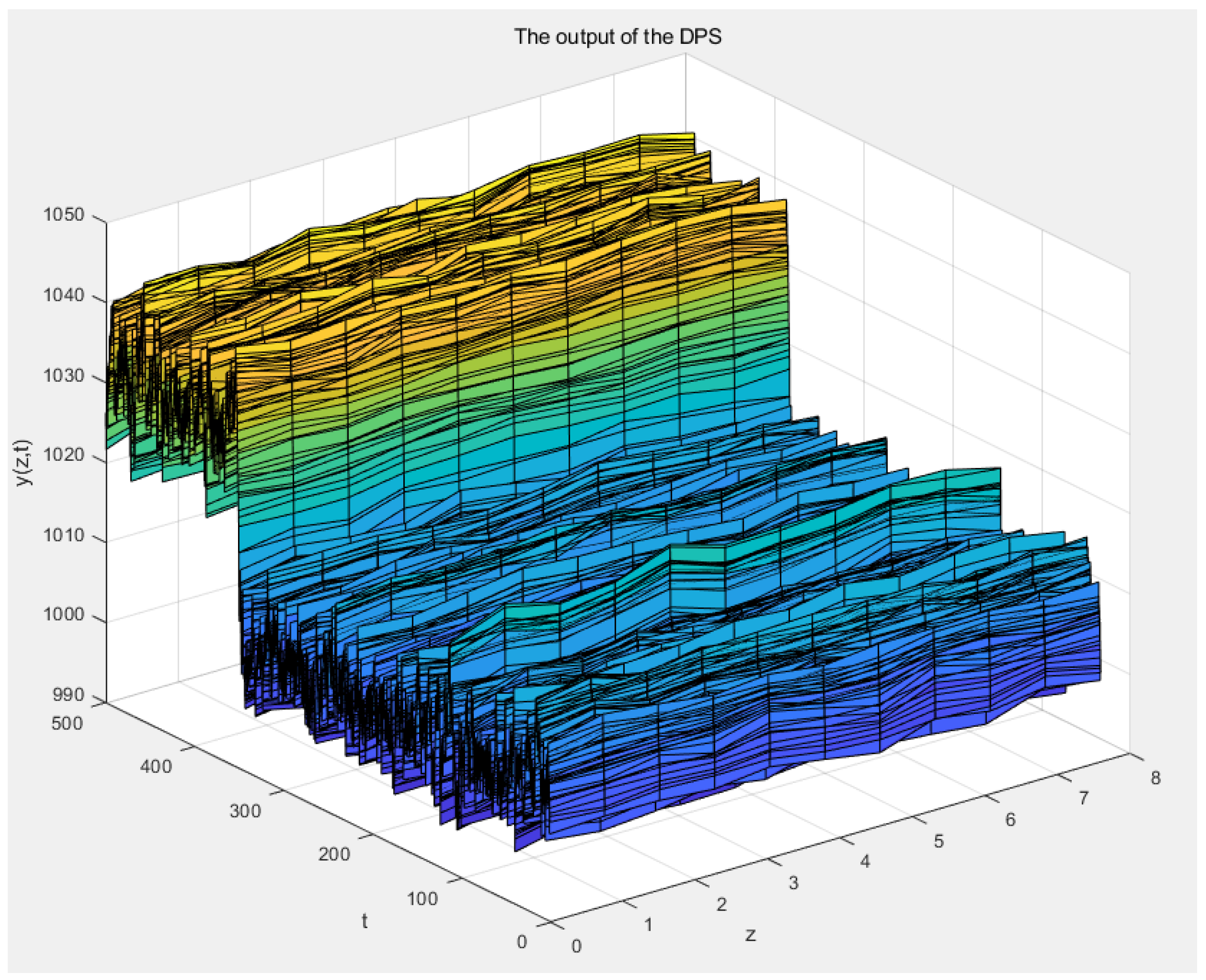The sample period was set as $\mathsf{\Delta }t=0.1s$ and the experiment lasted for 500 s. The data generated from the experiment are shown in Equation (60).

$$S=\{x^k,y_z^k\}=\{(x_z^k,x_u^k),y_z^k|x_z^k\in R^{11\times 1},x_u^k\in R^{1\times 3},y_z^k\in R^{P\times 1},k=1,\cdots ,5000\}$$

(60)

where,

$x^k=(x_z^k,x_u^k)$;

$x_z^k=\left[T(\overline{Z},k-1)\right]$;

$x_u^k=[u_a(k-1),u_b(k-1),u_c(k-1)]$;

$y_z^k=T(\overline{Z},k)=[T_f(f_1,k),\cdots ,T_f(f_{11},k)]$.

Unlike offline modeling algorithms, online modeling algorithms use data generated in real-time by the DPS simulation system. At a given time t, the 3DFDPG model predicts the output at time t based on the output and input of the DPS system at time $t-1$, as shown in Equation (61).

$$y\left(t\right)=f\left(y\right(z,t-1),u(t-1),\theta )$$

(61)

The hyperparameters for the 3DFDPG are specified in

Table 1. The hyperparameters of the 3DFDPG.

Parameters	Value	Description
Mini-batch Size	20	Mini batch Size
Buffer Size	40	Replay buffer size
Num of the Q value function 3D fuzzy rules	20	The number of the Q value 3D fuzzy rules
Num of the policy rules	20	The number of policy 3D fuzzy rules
${\alpha }_1$	0.001	Critic’s learning rate
${\alpha }_2$	0.001	Actor’s learning rate
${\beta }_1$	0.9	The hyperparameter for exponential decay in the Adam optimizer
${\beta }_2$	0.999	The hyperparameter for exponential decay in the Adam optimizer
$ϵ$	1 × 10−8	Adam’s stability constant

.

In this paper, we use Matlab2023b software to realize the simulation of RTCVD, the realization of 3D fuzzy modeling, and the comparison of different modeling methods.

4.1. Simulations

Ideally, an off-line model based on the historical data with sufficient information can show the dynamic characteristics of the actual system well. However, when the dynamic characteristics of the actual system change, such as equipment aging, local equipment damage and large changes in operating conditions, the off-line model cannot express the dynamic characteristics of the change. However, an online model makes up for this deficiency. In this study, two scenarios of the RTCVD system are investigated to simulate external or internal environmental changes, including change in the system’s radiation coefficient ${\sigma }_0$ and change in wafer density $w_0$.

(1) The parameters ${\sigma }_0$ are changed

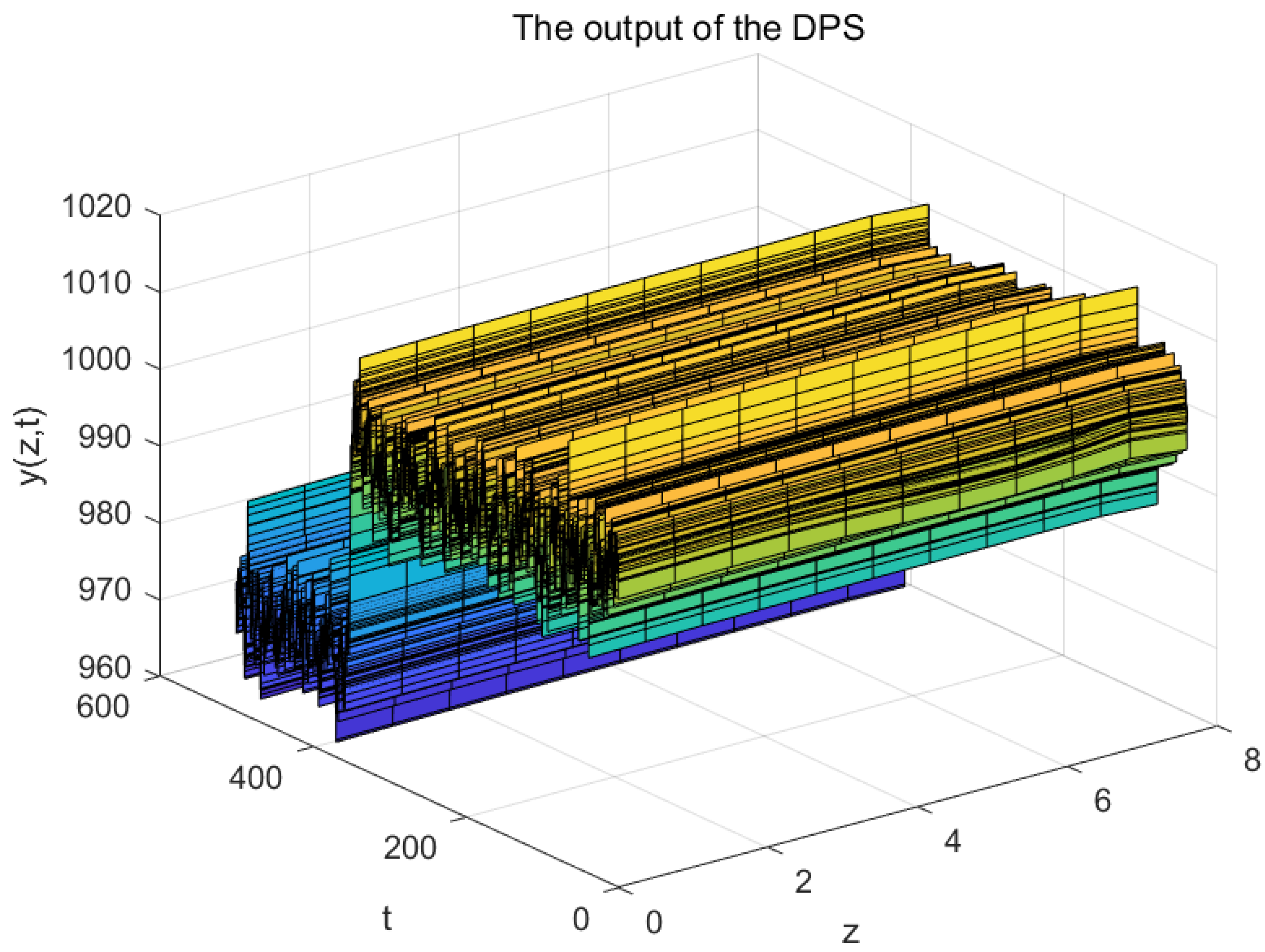
Parameters ${\sigma }_0$ are reduced by 10% after 350 s to simulate the external change of the real system environment. To illustrate the modeling performance in response to changes in the DPS’s circumstances, we show the 400 data between 330 s and 370 ts.

As shown in Figure 8, when the system’s radiation coefficient ${\sigma }_0$ decreases, heat diffusion in the furnace slows down, causing a sudden temperature increase in the system, After a certain period, the system’s temperature stabilizes, that is the DPS’s actual output $y(\overline{Z},t)$. As the predicted output $\widehat{y}(\overline{Z},t)$ illustrated in Figure 9, the model established in this paper is able to follow this change in the system. Figure 10 shows that the higher the immediate reward, the higher the model’s accuracy, with the peak reaching 0 at around 60 s, indicating that the proposed online modeling method has high modeling efficiency. 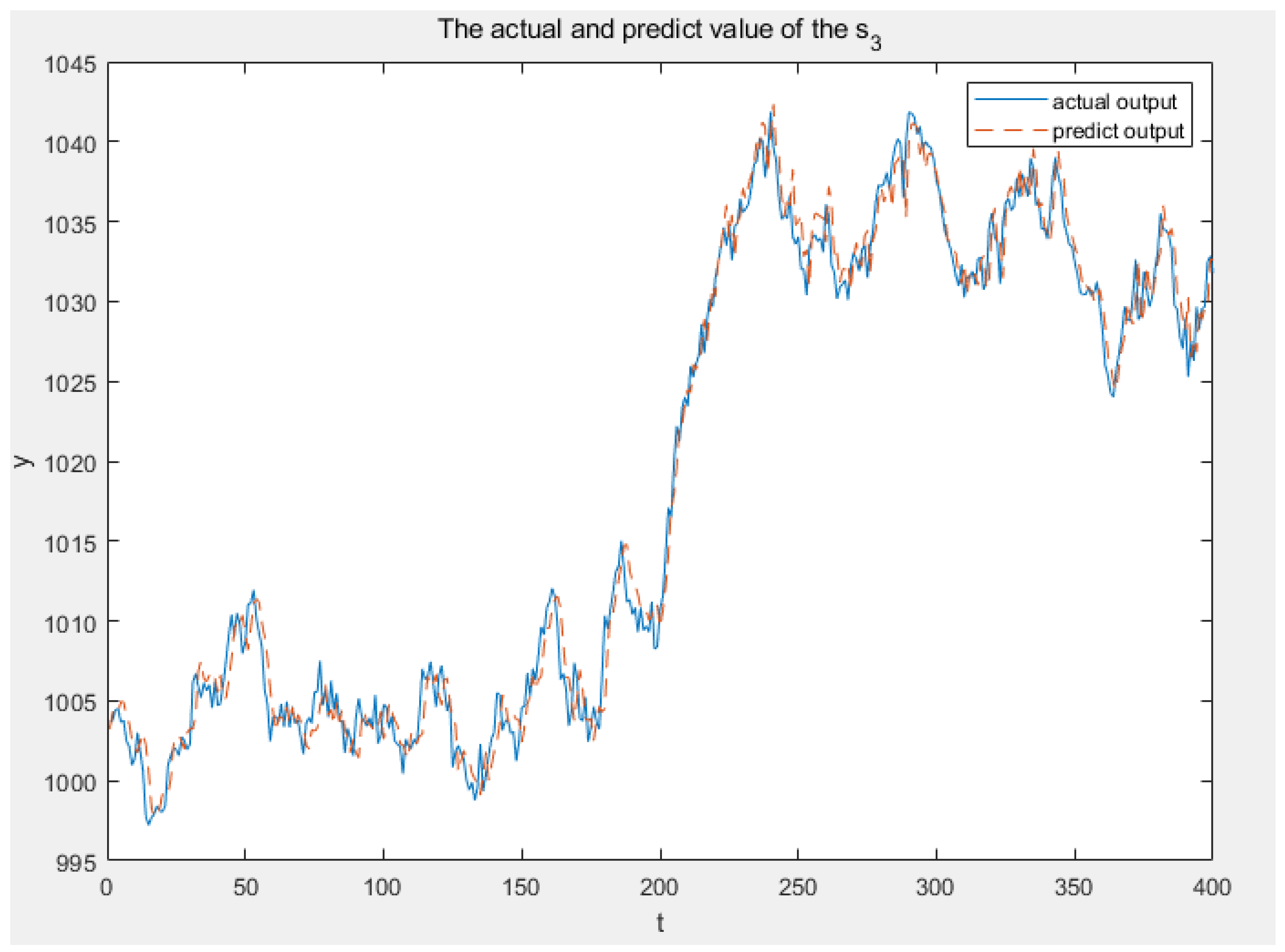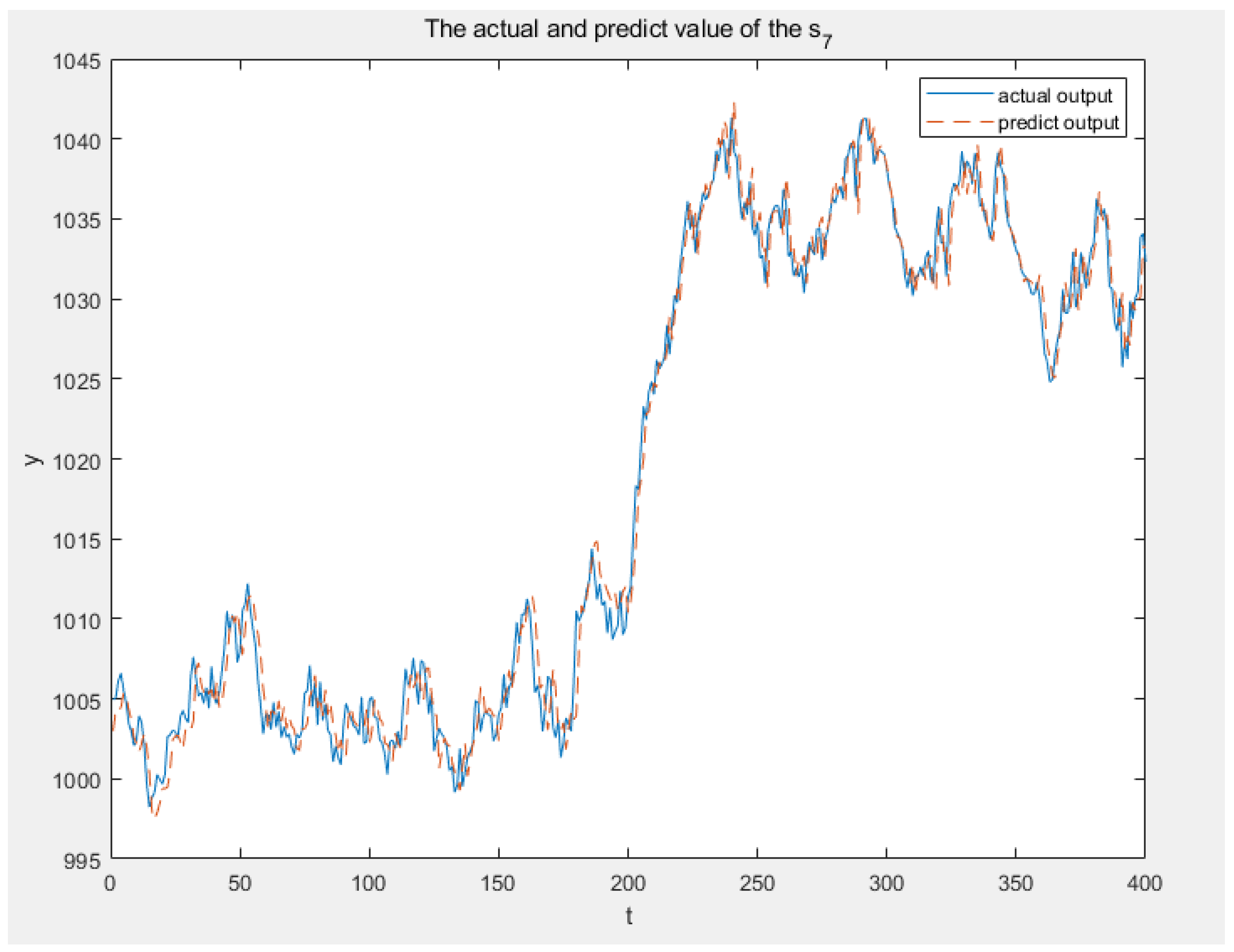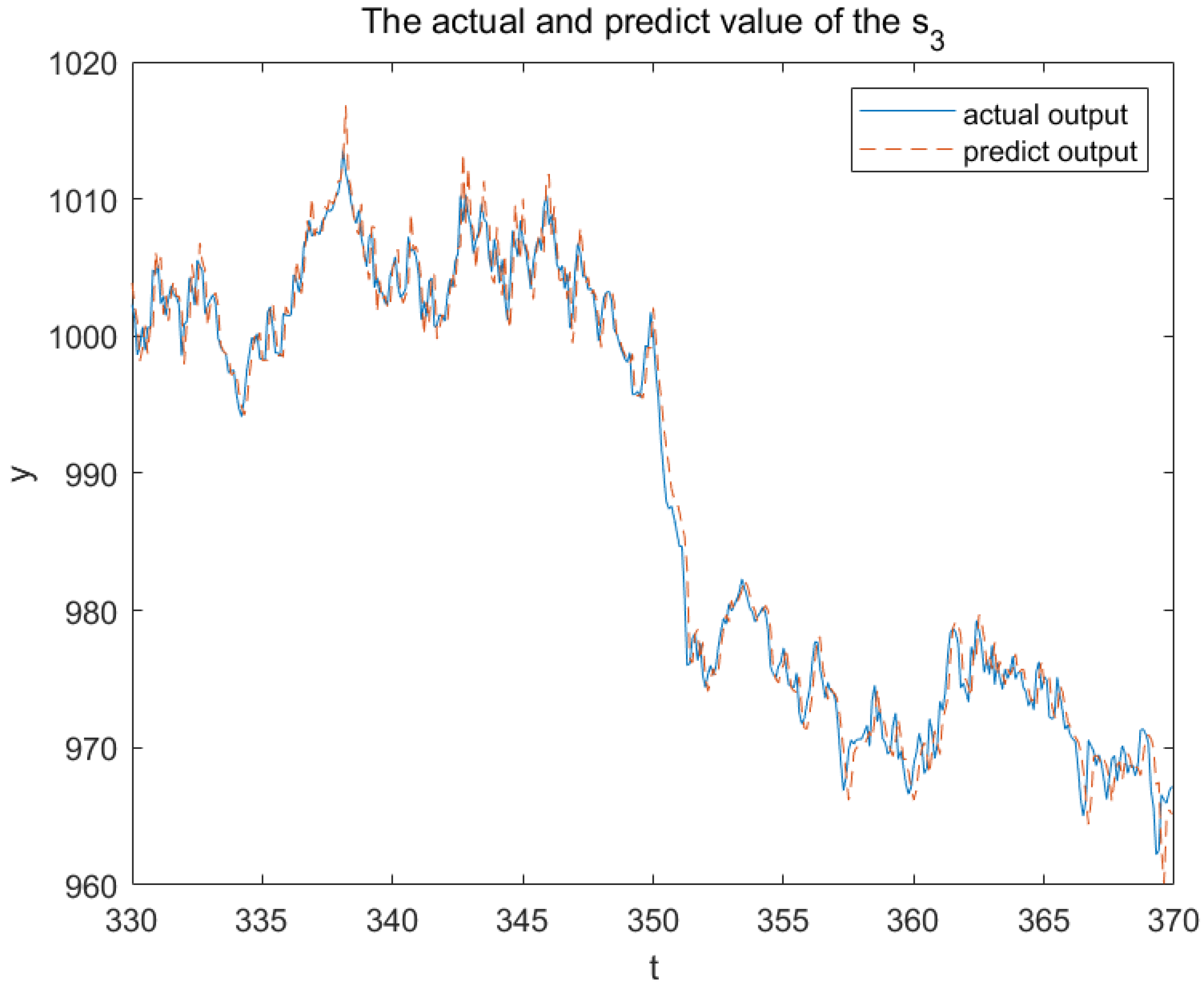Figure 11, Figure 12 and Figure 13 illustrate the real and anticipated values from sensors $s_3$, $s_5$ and $s_7$, respectively, to elucidate the modeling accuracy of 3DFDPG under varying system conditions. It can be seen from the figures that the 3DFDPG model can promptly track changes in the system, proving the effectiveness of the proposed modeling method. 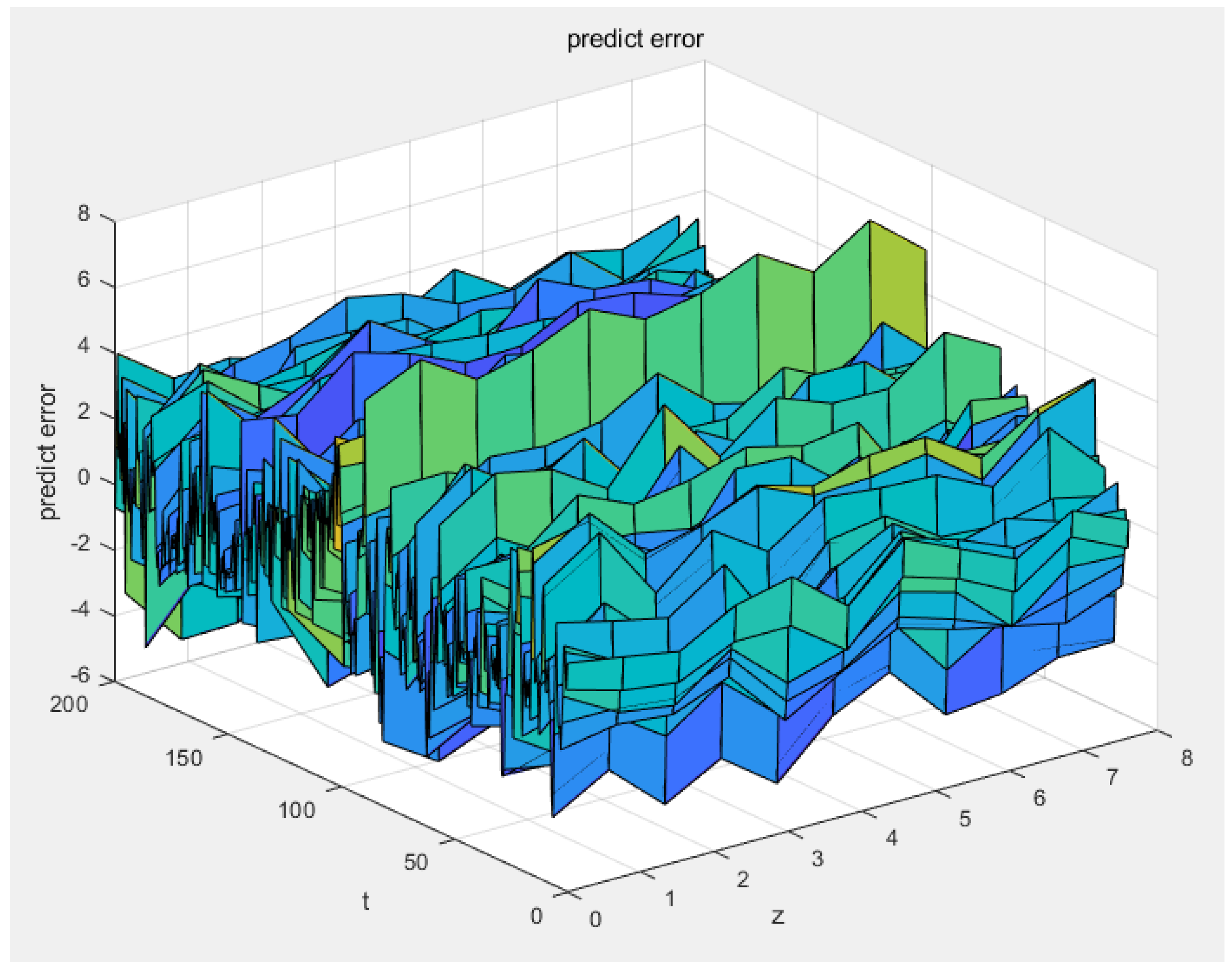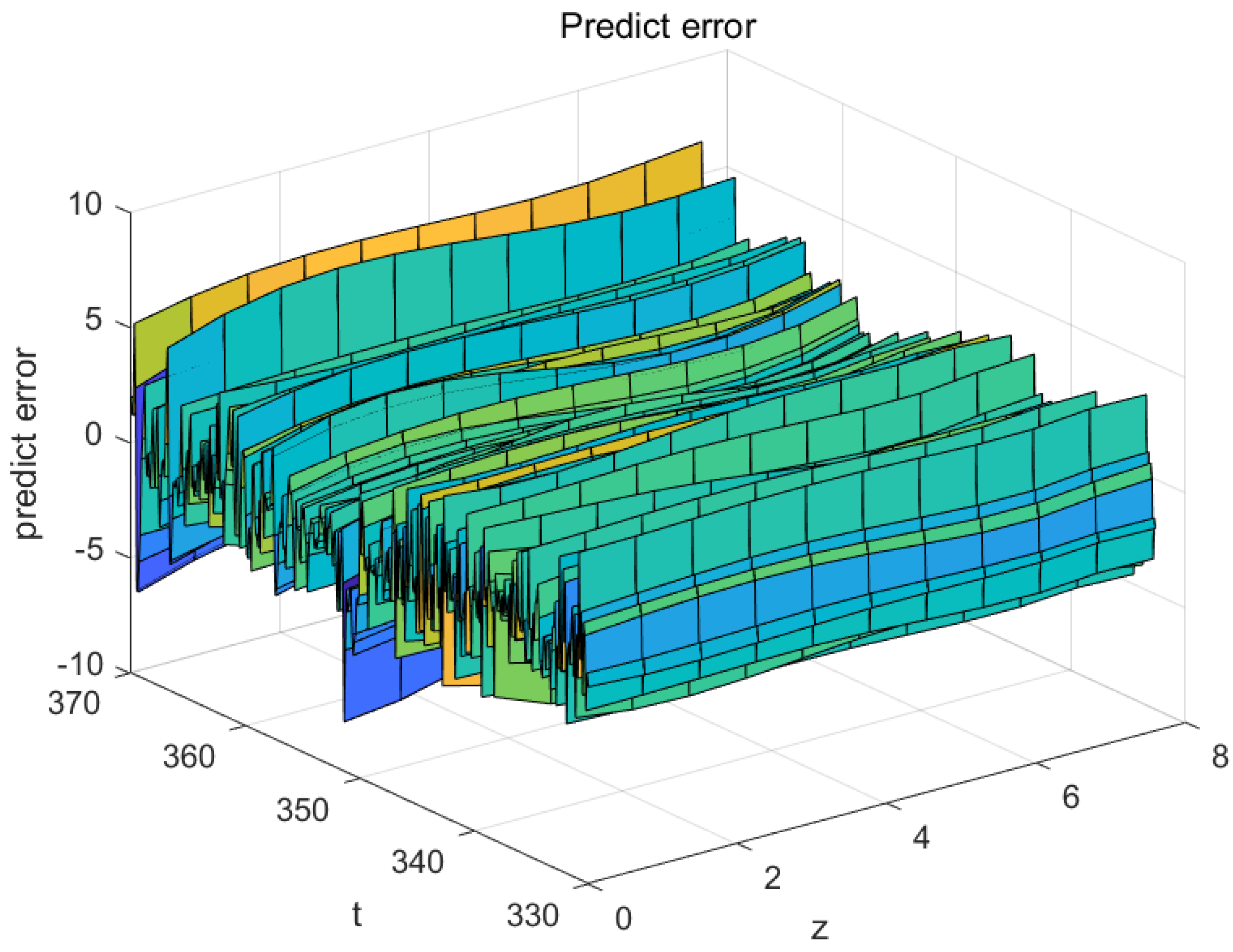Figure 14 and Figure 15 illustrate the prediction error and relative error of the 3DFDPG method, with the prediction error spanning from [−6, +6] and the relative error measuring 0.006. It indicates that the proposed online modeling method has good model accuracy.

(2) The parameters $w_0$ are changed

Parameters $w_0$ are reduced by 10% after 350s to simulate the internal change of the real system environment. To illustrate the modeling performance in response to changes in the DPS’s circumstances, we show the 400 data between 330s and 370s.

As shown in Figure 16, when the wafer density $w_0$ decreases, the wafer temperature drops, causing a sudden decrease in the system’s temperature, which then stabilizes after reaching a certain level. As illustrated in Figure 17, the model established in this paper is able to follow this change in the system. Figure 18 illustrates that an increase in immediate reward correlates with enhanced model accuracy, peaking at 0 around 60 s. This indicates that the proposed online modeling method has excellent modeling efficiency. Figure 19, Figure 20 and Figure 21 correspondingly illustrate the actual and expected values from sensors $s_3$, $s_5$ and $s_7$. These figures indicates that the 3DFDPG model can swiftly monitor system changes, hence validating the efficacy of the proposed modeling method. Figure 22 and Figure 23 illustrate the prediction error and relative error of the 3DFDPG algorithm, with the prediction error spanning from [−6, +6] and the relative error at 0.006. This indicates that the proposed online modeling method maintains commendable model accuracy despite variations in wafer density $w_0$.

4.2. Comparison and Analysis

The accuracy of the model is measured by relative error, the time normalized absolute error (TNAE) and the relative L2 standard error (RLNE) as Equations (62), (63) and (64), respectively.

$$Relativeerror=|{\displaystyle \frac{\widehat{y}(\overline{Z},t)-y(\overline{Z},t)}{y(\overline{Z},t)}}|\times 100\%$$

(62)

$$TNAE\left(\overline{Z}\right)=\sum |\widehat{y}(\overline{Z},t)-y(\overline{Z},t)|/\sum \mathsf{\Delta }t$$

(63)

$$RLNE\left(t\right)=(\int {(\widehat{y}(\overline{Z},t)-y(\overline{Z},t))}^{2}d\overline{Z}{)}^{1/2}/{(\int y{\left(\overline{Z},t\right)}^{2}d\overline{Z})}^{1/2}$$

(64)

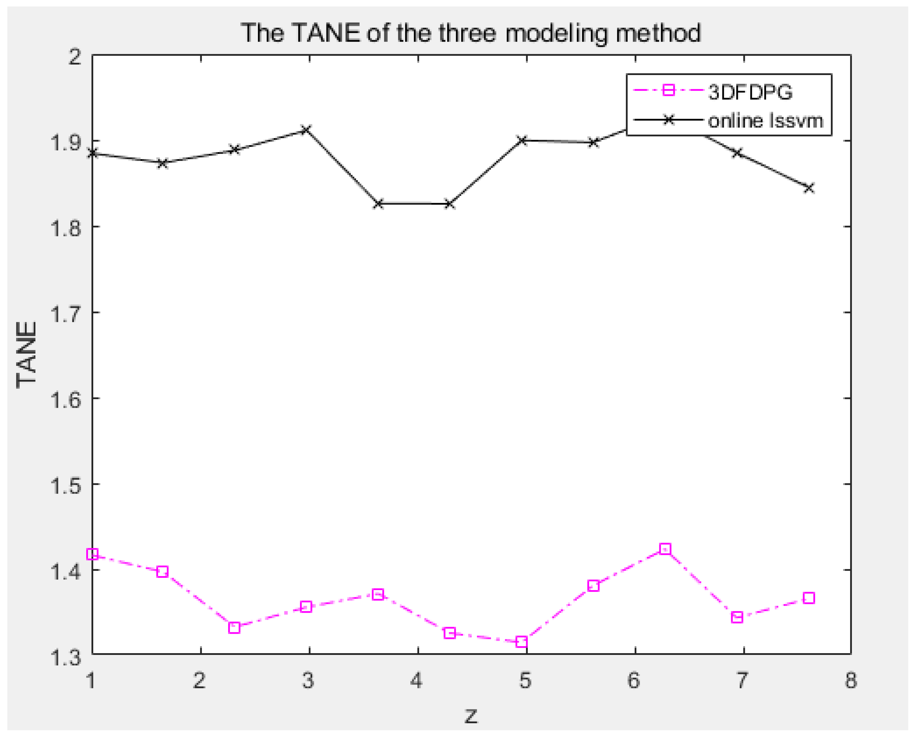
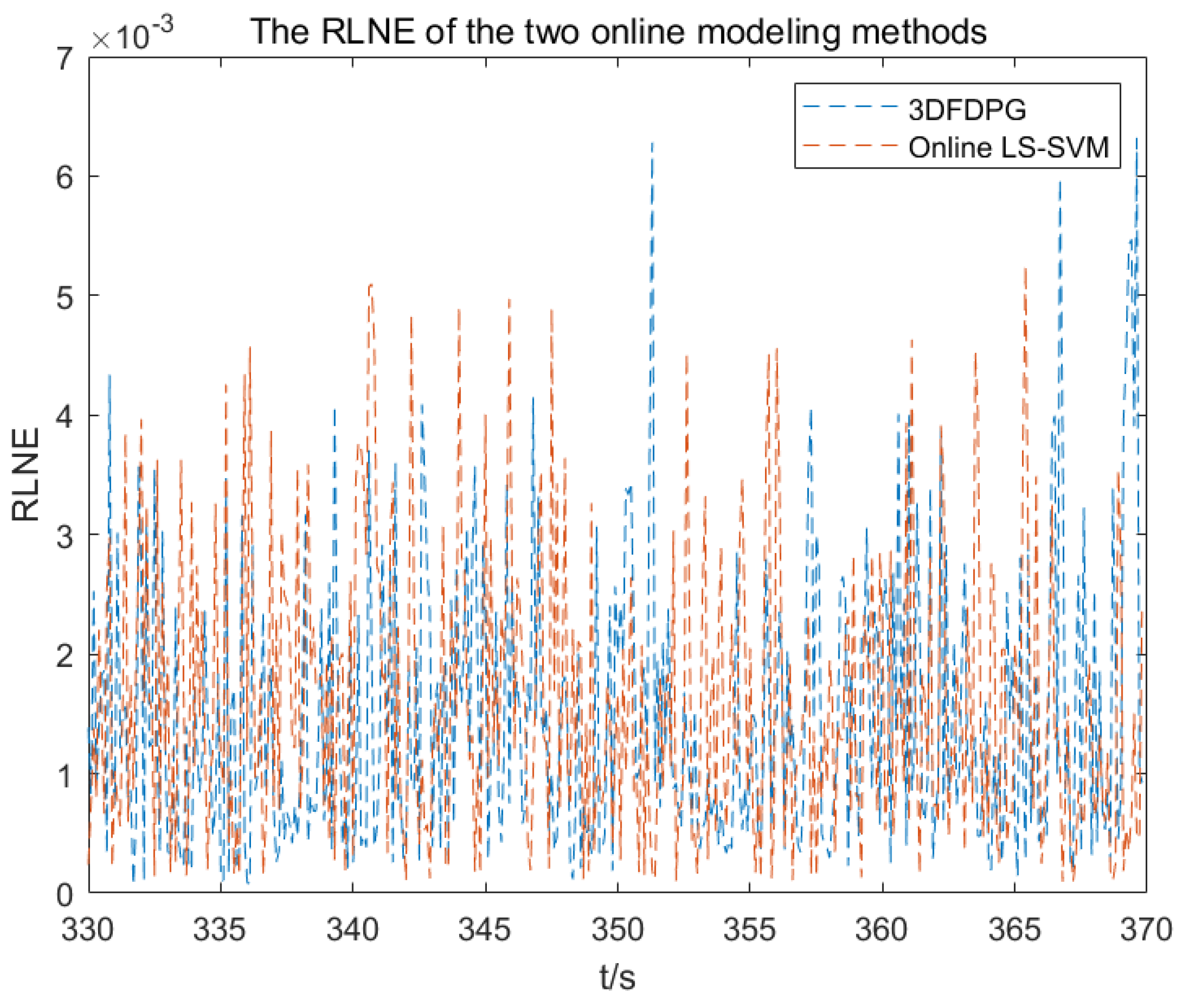
Then, we compared the proposed 3DFDPG with KL-LS-SVM [48] as a traditional offline DPS modeling method and online LS-SVM [28] as a newly proposed online DPS modeling method. Figure 24 and Figure 25 compare the TANE obtained from the two online modeling methods. Figure 26 and Figure 27 compare the RLNE obtained from the two modeling methods.

Table 2. Mean RMSE and its standard deviation of the three models.

Modeling Method	Mean RMSE with ${\mathit{\sigma }}_0$ Changed	Standard Deviation of RMSE with ${\mathit{\sigma }}_0$ Changed	Mean RMSE with ${\mathit{w}}_0$ Changed	Standard Deviation of RMSE with ${\mathit{w}}_0$ Changed
KL-LS-SVM	28.4719	0.03	29.9498	0.03
Online LS-SVM	2.31787	0.0417	2.0164	0.0454
3DFDPG	1.7686	0.0550	1.7915	0.0270

presents the mean RMSE and the standard deviation of the three models by changing the random seed and conducting 10 trials. In both cases, the modeling error of the offline model (KL-LS-SVM) is much larger than that of the other two online models. The offline model is unable to cover the data in the new scenario when the DPS’s circumstances change. But since the online modeling method uses incremental learning, it can still appropriately assess the DPS in different scenarios. In addition, we conduct t-test and p-value analyses for the two online modeling methods. The T-test calculation equation for the two online models is as follows:

$$T={\displaystyle \frac{{\overline{X}}_1-{\overline{X}}_2}{\sqrt{\frac{s_1^2}{n_1}+\frac{s_2^2}{n_2}}}}$$

(65)

where ${\overline{X}}_i$, $s_i$ and $n_i$ represent the mean of RMSE, the standard deviation of RMSE and the number of samples from the ith online model, respectively, $i=1$ represents the 3DFDPG model and $i=2$ represents the online LS-SVM model. Substituting the data from Table 2 into Equation (65) yields the T value. Then, we obtain the p value by consulting the corresponding statistical distribution table, that is T = −35.27, p < 0.01 with ${\sigma }_0$ changed and T = −13.47, p < 0.01 with $w_0$ changed. Since the p value is less than 0.05, we reject the null hypothesis and conclude that there is a significant difference between the means of the two groups. This demonstrates that the proposed 3DFDPG model outperforms the Online LS-SVM model under the two application scenarios.

TNAE and RLNE represent the prediction errors of the 3DFDPG model and the online LS-SVM model in spatial and temporal dimensions, respectively. As shown in Figure 24, Figure 25, Figure 26 and Figure 27, in both cases, the errors of the 3DFDPG model are smaller than those of the online LS-SVM model. The reason is that the 3D fuzzy system naturally achieves temporal-spatial separation and temporal-spatial synthesis, allowing for the spatiotemporal modeling of DPS without the need for model reduction. Therefore, the 3DFDPG modeling method outperforms the online LS-SVM model. The online LS-SVM updates its model from an initial offline model. In contrast, the proposed 3DFDPG starts from scratch, relying on the interaction between the agent and the environment, with model parameters being updated adaptively.

5. Conclusions

In this paper, we proposed a 3DFDPG modeling method for online modeling of the DPSs. Reinforcement learning is learning from interactions between an environment and an agent; the 3D fuzzy system has the ability to deal with spatiotemporal data and has the universal approximation property. The reinforcement learning algorithm and the 3D fuzzy system were combined to realize the online learning. The average reward set was utilized to implement the online modeling of the DPS, so that the modeling process can run forever and have the ability to catch the situation change of the DPS. The simulation results confirmed the efficacy of the proposed 3DFDPG algorithm and its exceptional modeling performance is further emphasized by comparison with existing DPS modeling methods.

Due to practical constraints, this paper applied the proposed 3DFDPG modeling method to an RTCVD simulation system, aiming to simulate the real system as closely as possible by varying parameters and adding disturbances. When applied to the real system, the benefits are as follows:

• It develops a very accurate model for the actual system to serve as a reference for system optimization, control and cost reduction.
• This work proposes an online modeling technique capable of swiftly indicating internal or external component failures inside the system, hence furnishing engineers with accurate fault-localization data.
• The proposed online modeling method can model the real system from scratch without human intervention, facilitating system modeling.

Although the proposed online modeling algorithm achieved good results, there are two limitations, which need to be solved in future work. Firstly, the 3D fuzzy system used in this paper has a fixed structure and lacks flexibility. In future work, a dynamic variable structure 3D fuzzy system will be investigated. Secondly, the reinforcement learning algorithm based on DPG used in this paper is somewhat insufficient in terms of action exploration and may become trapped in local optimal policies. In future work, the feasibility of using reinforcement learning algorithms based on stochastic policies will be explored. Finally, we plan to apply the proposed online modeling method to a real industrial system, for instance a rotary hearth furnace system.