1. Introduction
Robot navigation [
1] is an active topic of research due to the growing demands in sectors like retail services, manufacturing, logistic, healthcare, domestic services, and warehouse management [
2]. For many tasks, a mobile robot is required to follow a set path or prescribed route from a start location to destination location or locations. For example, a waiter robot has to go from the kitchen to the customers to deliver food. An autonomously guided vehicle robot needs to traverse between various assembly stations to autonomously deliver parts. Service robots operating in a hospital need navigation to transport food and medication throughout the premises. Cleaning robots need sophisticated techniques to navigate within their service area. The basic parameters of the robot’s movement in reaching its destination include speed, positioning accuracy, the type of movement trajectory (e.g., linear), etc. [
3]. These are the essentially similar regardless of whether the robot is mobile (e.g., an automated vacuum cleaner) or stationary (e.g., an industrial robotic arm for assembling). These parameters need to be considered while developing a system for controlling a robot.
Outdoor navigation can utilize Global Positioning System (GPS) for robust real-time applications. However, GPS does not function reliably inside buildings due to the degradation of the satellite signals caused by obstructions. Popular methods for robot navigation in an indoor environment include simultaneous localization and mapping (SLAM), and utilizing the information acquired by its onboard sensors like an odometry sensor, inertia measurement unit (IMU), ultrasonic sensor, electronic compass, light detection and ranging (LiDAR) sensor, and camera [
4]. While such techniques are quite mature, robot navigation based on indoor positioning systems (IPSs) has started to get the attention of researchers in recent times [
5]. This is driven by the rapid advancement in indoor localization [
6] that, apart from robot navigation, can potentially be used for asset tracking, and smart guidance in large facilities like airports. Proprioceptive sensors (IMU, odometry) are subject to cumulative errors [
1]. Kidnapped robot or locomotion failure can also create issues as the current location information is lost [
7]. Therefore, a global localization-based solution using IPS also offers some inherent advantages by not being susceptible to these issues.
The most common IPSs are based on radio frequency technologies like Wi-Fi [
8], BLE [
9], ultra-wide band (UWB) [
10], and radio frequency identification (RFID) [
11]. However, their relatively low localization accuracy means that they are more suited as a secondary source of information for sensor fusion-based navigation [
12]. In contrast technologies which offer centimeter-range indoor positioning accuracy such as acoustic signals and visible light signals hold more promise for robotic navigation. Visible light positioning (VLP) has the comparative advantage of being able to leverage pre-existing lighting infrastructure. Light-emitting diodes (LEDs), which are energy efficient, long lasting, and emit low heat, are rapidly becoming the preferred technology for modern indoor lighting infrastructure. The abundance of pre-installed LED lightings presents opportunity to simultaneously use them for visible light communication (VLC) [
13] and VLP.
2. Related Work
In VLP systems, LED luminaires are used as the transmitting beacons with either a photo diode (PD) or camera as the common receiver sensor attached to the tracked object. Both sensors come with inherent advantages and disadvantages. While cameras may allow for more sophisticated communication schemes [
14], PD-based receivers are considerably cheaper and energy efficient [
15], and incur less computational cost [
16]. Received signal strength (RSS) is the most widely utilized signal characteristic for a PD-based VLP due to simplicity and convenience [
17]. VLP that utilizes RSS can either be model- or fingerprinting-based [
18]. Fingerprinting-based methods can be time- and labor-consuming compared to the model-based ones. Considering all these points, the VLP system used for this work employed a PD-based receiver that utilizes RSS as the signal characteristic and localizes using a model-based technique. A literature review shows many localization works based on a PD-based receiver utilizing RSS (for example, see the recent survey paper by Rahman et al. [
19] on VLP) achieving centimeter-level accuracy. However, there is no reported work that uses such a VLP system as the singular tool for controlling robots in real time.
A survey of recent literature on VLP-based indoor robot navigation yields only a handful of papers. These works utilize a rolling shutter effect (RSE) camera as the light sensing device (please see [
20,
21,
22] for examples of RSE-based VLP systems). Though the method uses more computer computation time and a complex algorithm because of the involvement of image processing and classification algorithm, the availability of ubiquitous CMOS image sensor cameras in most smartphones has made them the preferred choice among researchers.
Rátosi and Simon [
23] employed an RSE camera installed on a mobile robot to determine its pose from the signal received from modulated LED luminaires. While the system is shown to be able to track the moving robot in real time in a 6 m × 6 m room within a low centimeter range, the VLP system is not used for the navigation. The process of decoding LED-ID information from the captured images using an RSE camera can be slow due to the computational latency. Therefore, Li et al. [
24] proposed using convolutional neural network (CNN) to increase the speed of identifying the anchor node ID from the captured image, especially with motion blur caused by the fast movement of a robot.
Hua et al. [
25] proposed the fusion of a PD- and camera-based system using a version of the Kalman filter. The system is shown to be robust and has the ability to perform real-time positioning. However, the system was not used to control or navigate a robot. Amsters et al. [
16] demonstrated the capability of a PD-based VLP that utilizes only unmodulated light. While their system has the potential to estimate the pose of a mobile robot, the experimental results do not show real-time position estimation. They also do not control or navigate the robot using VLP. Zhuang et al. [
26] reported on a PD-based VLP system that may be used for the localization of a mobile robot. However, the article only reports localization accuracy; the VLP system is not used to control the movement of the robot.
Guang et al. [
5] proposed indoor robot localization based on a VLP system that utilized an RSE camera installed on Turtlebot 3 running a robot operating system (ROS). They presented an extension [
27] of this work by introducing a loosely coupled multi-sensor fusion with LiDAR- based SLAM and odometry. Another improvement [
28] of the work involves the fusion of VLP and IMU to improve the system’s robustness with the ability to handle luminaire shortage/outage. A similar work on the fusion of VLP and IMU to address luminaire shortage/outage issues for an RSE-based receiver can be found in [
29]. It should be noted that only one of the articles [
28] develops a method for controlling the robot, whereas the other two articles [
27,
29] focus mainly on the localization aspect.
Therefore, a clear gap in the state of the art can be seen. There is a noticeable lack of works that utilize VLP for controlling a robot. Recent literature shows only a small number of works on robots being controlled by fusing location information acquired via VLP that uses an RSE camera as a receiver with other sensor data. There is no reported work that has used only PD-based VLP to control a robot. This is the motivation of the work being presented in this article.
3. Contribution
As far as the authors are aware of, this is the first reported work that utilizes only a PD-based VLP system to control the movement of a robot. In this work, two novel algorithms are proposed and implemented to control the movement of a cartesian robot, constructed in the form of a 2D Computer Numerical Control (CNC) machine, solely by a VLP system in real time. This also allowed for objectively evaluating the efficacy of a PD-based VLP system for controlling a robot. Based on the experimental results collected while the robot is traversing multiple path patterns, both algorithms show promising accuracy.
This is how the rest of the article is organized.
Section 4 describes the experimental setup and bespoke hardware. The visible light positioning technique and calibration of the VLP system are discussed in
Section 5. The algorithms for controlling the movement of the robot are developed in
Section 6. Experimental results are presented and discussed in
Section 7. Finally,
Section 8 concludes the paper and identifies some potential work that can be carried out to extend the research.
4. Experiment Setup
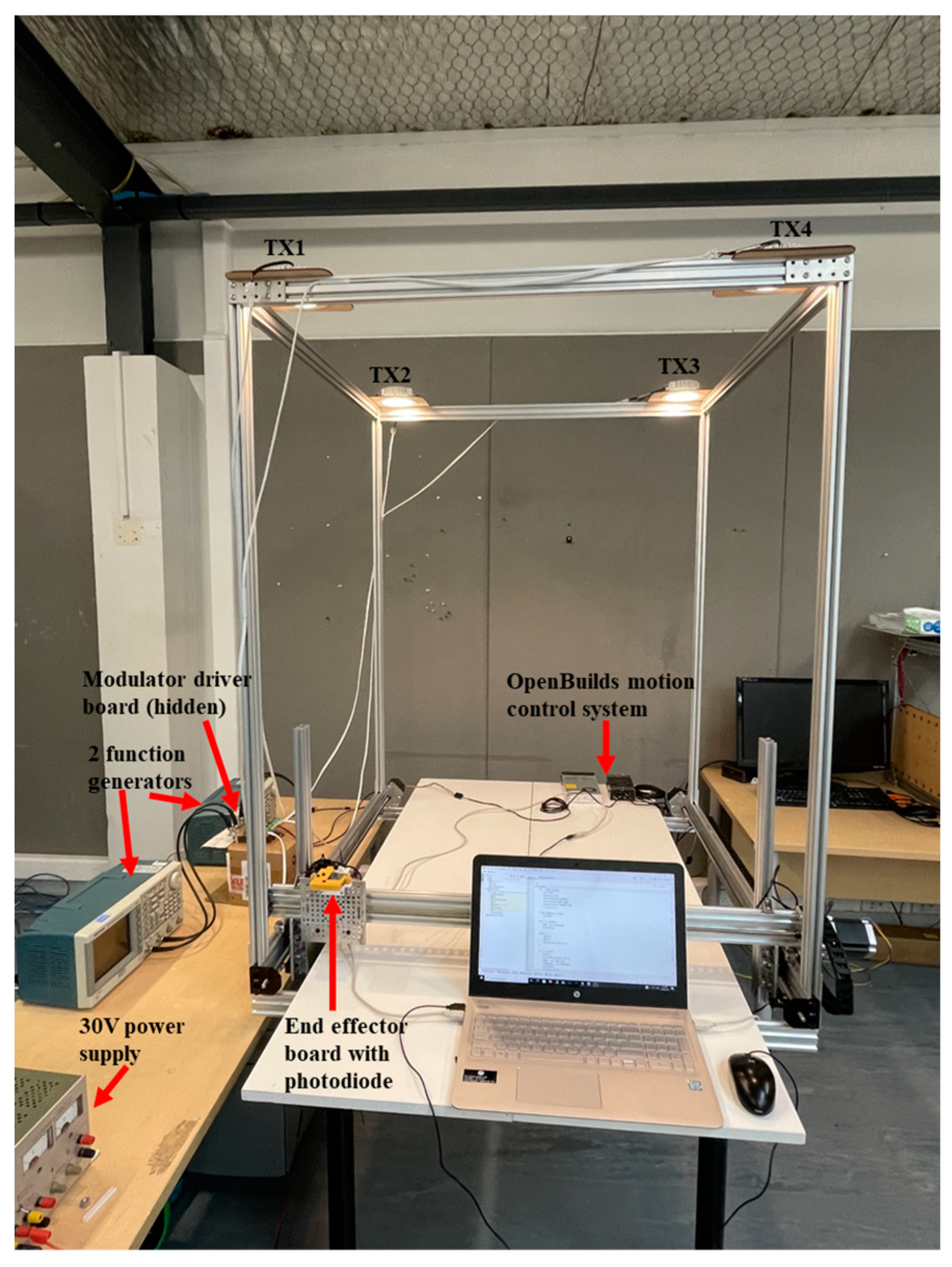
The key equipment of the experimental setup is a purpose-built 2D CNC machine (see
Figure 1). The VLP photodiode receiver is mounted on the end-effector. The CNC machine performs three important tasks:
It acts as the online robotic platform where the end-effector is driven by the VLP system;
The encoders of the CNC measure the X Y linear movement at the rate of 1000 mm per minute;
During the online phase, the CNC also records the exact locations of the receiver (end-effector). The location information is not used by the VLP system to drive the CNC, but it is used as the ground truth so that the localization accuracy or error statistics can be computed;
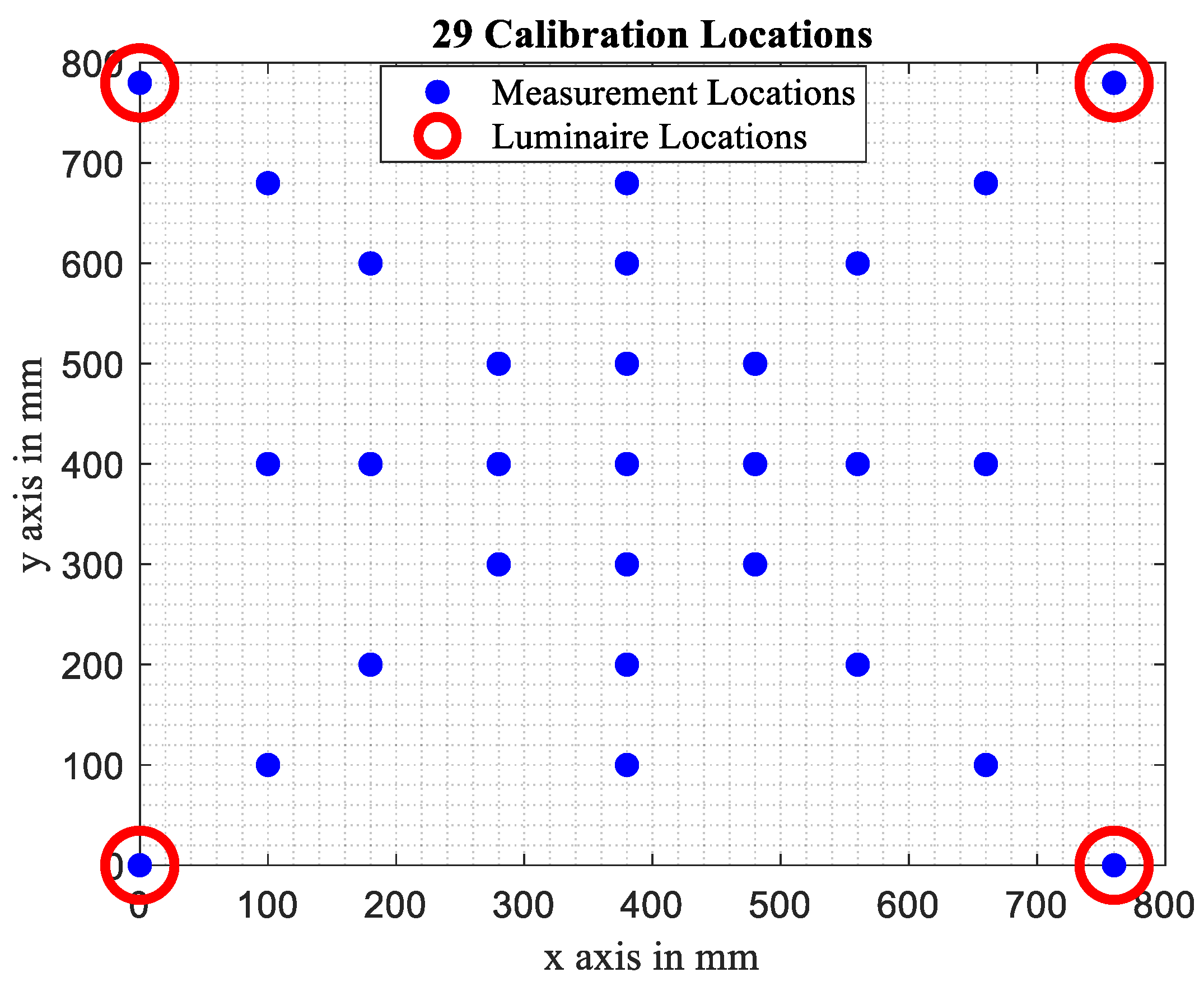
During the offline phase, the CNC is used to accurately position the VLP receiver at 29 pre-determined locations to collect RSS data for calibrating the Optical Propagation Model of the VLP system.
The end-effector’s minimum step size is 0.1 mm, achieved through lead screw actuation and Nema 23 stepper motors. An OpenBuilds BlackBox Motion Control System (MCS) with Grbl firmware controls the stepper motors. The host PC sends commands to the BlackBox MCS over a USB, with desired positions converted into GCODE commands via a Python program. These desired positions were computed by the VLP.
The VLP system consists of four transmitters constructed with LED luminaires which are commercially available and can be bought easily off the shelf. These luminaires are placed at a 1050 mm height above the CNC at known x–y locations: TX1 (0, 0), TX2 (0, 780), TX3 (760, 780), and TX4 (760, 0) (see
Figure 1).
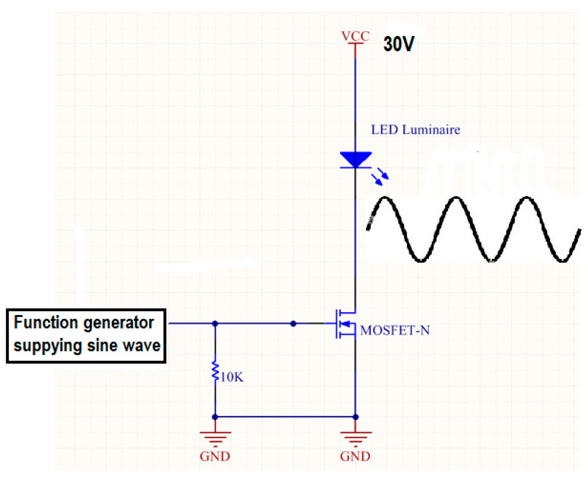
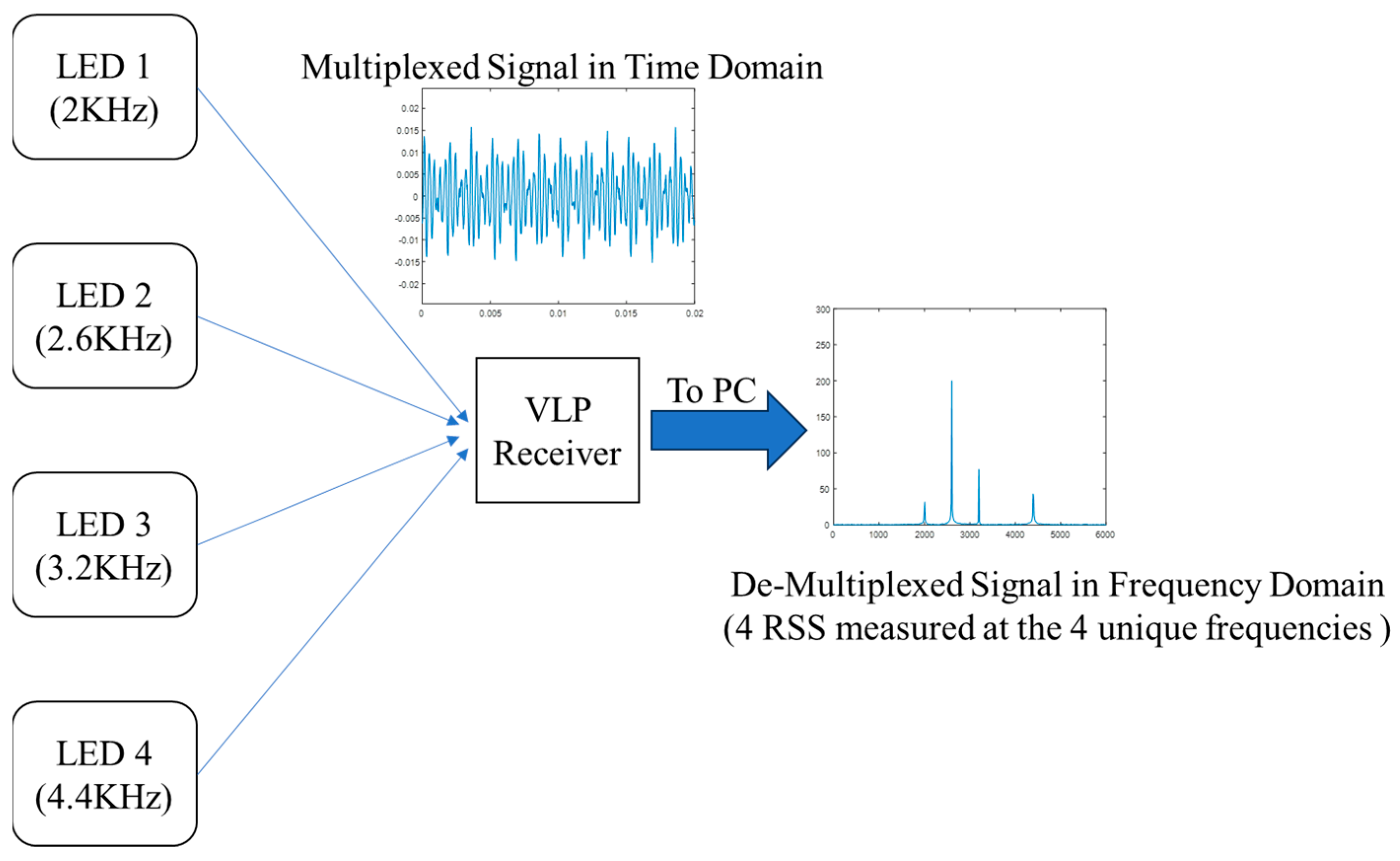
For the experiments conducted, an unmodulated sine wave of frequencies of 2 kHz, 2.6 kHz, 3.2 kHz, and 4.4 kHz were inserted by a modulator driver circuit powered by a 30 V power supply (shown in
Figure 2). The input of the modulator circuit is connected to a function generator which supplies the required sine wave. Each function generator has two signal generation channels. Altogether, two function generators are sufficient for this experiment (as seen in
Figure 1).
Underneath, the PD-based VLP receiver was mounted on the end-effector of the CNC. Together they form the robot that is controlled by utilizing the location estimated with respect to the fixed luminaires. On the receiver board, the photodiode sensor converted the optical signal to an electrical signal which was then amplified through a transimpedance amplifier before being processed by an onboard analog to digital convertor (ADC). More details of the receiver board can be found in [
30]. The sensor board receives and decodes the identities of these four lights using a Python program in the PC. After that, the data are transmitted out serially via USB to PC for Fast Fourier Transform (FFT) processing. The function of the FFT is to demultiplex and measure the magnitude of the four sinewaves present in the received signal [
30]. The magnitude squares constitute the RSS set at each location. Please refer to
Figure 3 for more details of the operation of the VLP system.
5. Localization Using VLP
During the offline stage, the RSS–distance relationship is found by calibrating the Lambertian propagation model. RSS data are collected at a set number of pre-determined locations for the parameter calibration. During the online phase, the live RSS readings are used to find the distance of the target device (the receiver on the end-effector) from each transmitter by “inverting” this calibrated propagation model. Subsequently, the receiver’s position is estimated via lateration.
5.1. Offline Calibration of VLP
For this research, the receiver/target plane and luminaire/transmitter plane are kept horizontal with respect to one another. This allows for the simplification of the Lambertian propagation model [
18]. Please refer to the discussion in
Section 8 on how this limitation can be addressed in the future.
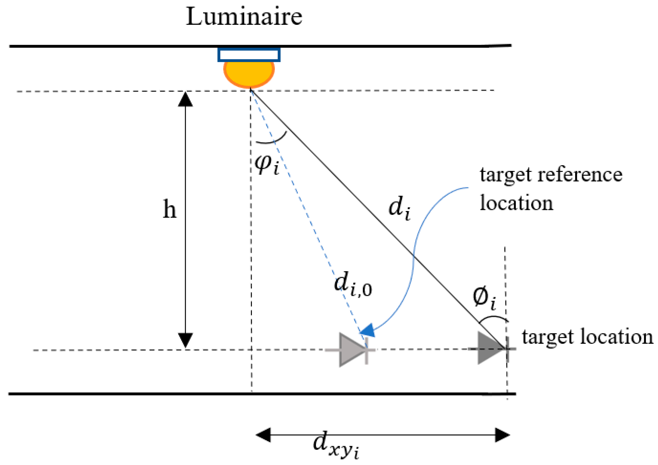
Under this assumption of a parallel arrangement, the received power,
, or the RSS at a distance
from the
luminaire (
Figure 4) within the field of view of the luminaire can be simplified from the Lambertian propagation model following the process outlined in [
18].
Here,
mi is the Lambertian order and
is the RSS at a
reference location at a distance
from the target. Equation (1) can be rearranged so that
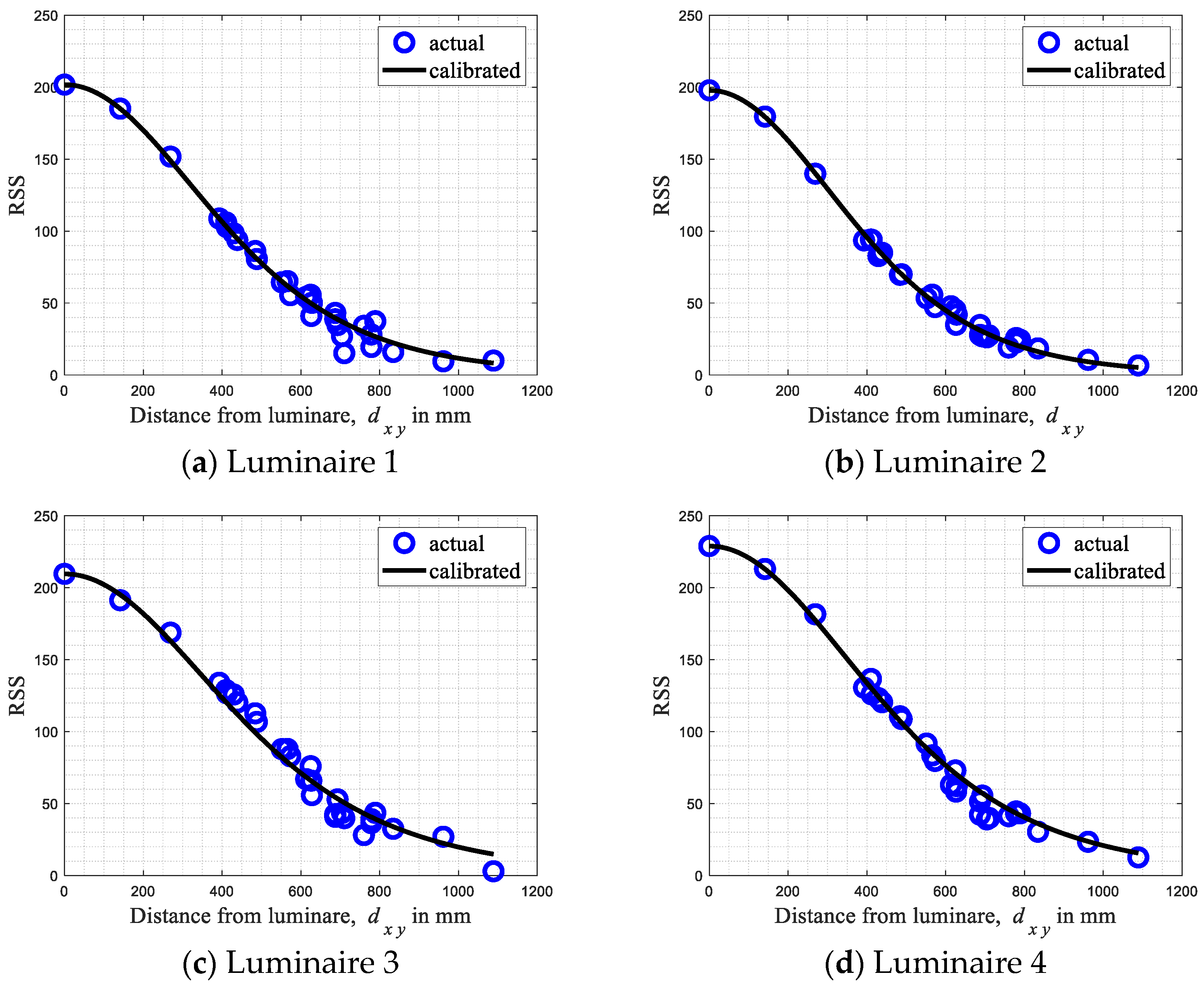
Figure 5 shows the position of the 29 offline locations where the RSS values were collected to estimate
for calibrating the RSS–distance relationship. As suggested by [
31], the reference location is chosen directly underneath the corresponding luminaire. The Lambertian order is estimated at the rest of the 28 locations using Equation (2), and then averaged over these 28 values. These offline locations are carefully chosen so that all regions of the Lambertian propagation models for each luminaire are captured [
32].
Table 1 shows the estimated Lambertian order and
Figure 6 shows the measured RSS values and the calibrated RSS–distance Lambertian curves of the four luminaires.
5.2. Online Localization Using VLP
Once the RSS–distance model is calibrated for each luminaire, Equation (1) can be rearranged for ranging (i.e., to compute the distance of the target from a luminaire) so that
The horizontal distance of the target from the
ith luminaire,
(please see
Figure 4) is computed as
6. Online Navigation
We developed two algorithms that can guide the end-effector to move from a starting point to the target/destination point(s). Both algorithms drive and make the end-effector move in a discrete manner, determined by the step size.
At each iteration of the algorithm, (1) visible light signal is captured by the VLP receiver (for 500 ms) and sent to the PC for extraction of RSS, (2) the distance of the end-effector from each luminaire is determined (as per the procedure discussed in the previous section), and (3) the end-effector is instructed to move by a step size toward a direction as determined by the algorithm or to remain stationary if the destination is reached. To maneuver the CNC machine, a GCODE set is needed to be sent to the OpenBuilds BlackBox motion control driver. The main program which is written in Python works out the x and y direction step movement from the algorithm and generates the equivalent steps in GCODE. The Black box motion control driver then processes the given GCODE and commands the movement of the stepper motors connected to the CNC machine.
6.1. Algorithm 1
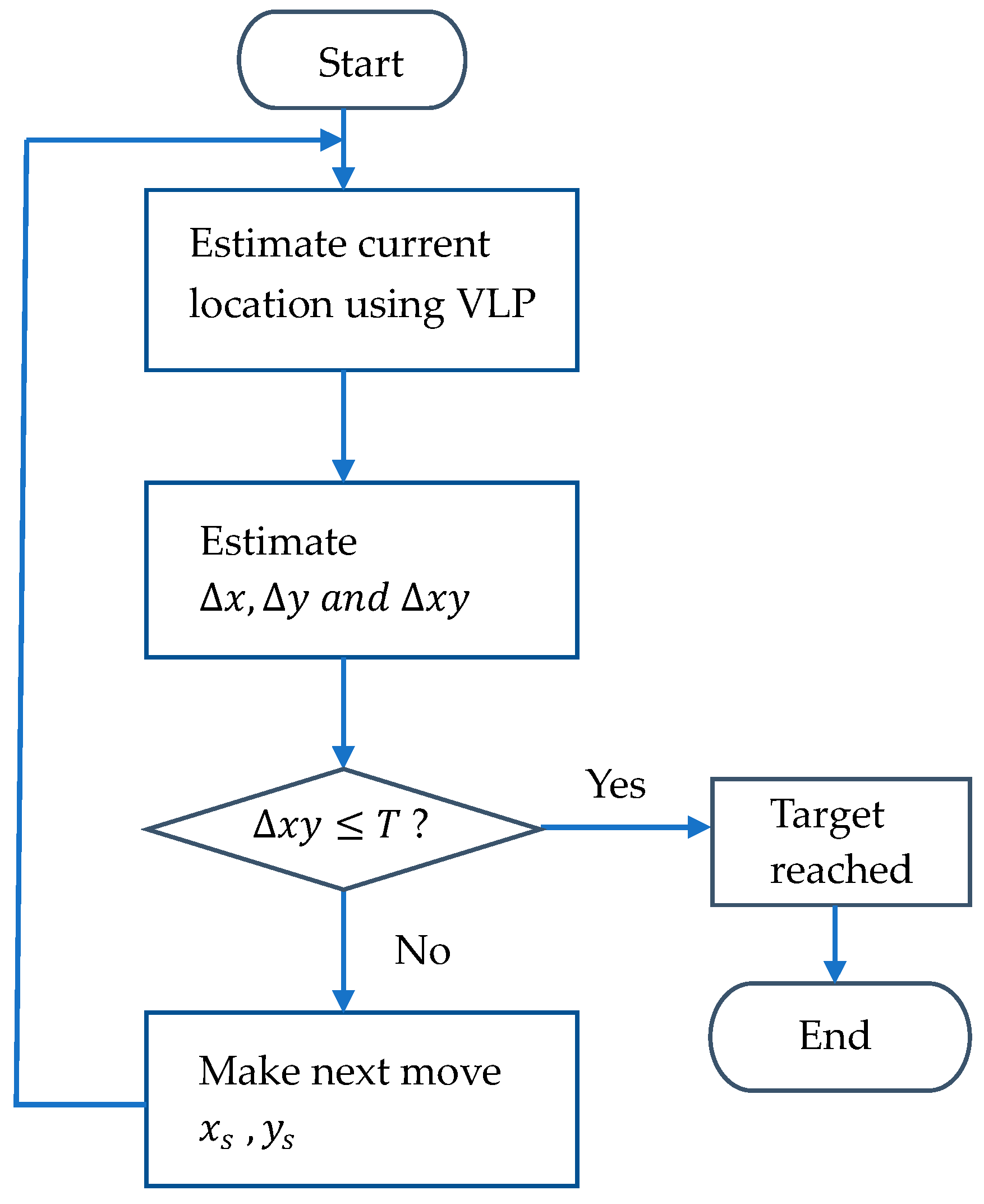
The flowchart in
Figure 7 shows the algorithm. The robot, if required, moves at a step size of
T. However, before any movement takes place,
- (i)
The robot’s current distance from each luminaire’s position is determined using live VLP reading following the process outlined in
Section 5.2. Once the horizontal distance of the target from all four luminaires is found, the location of the target on the xy plane is estimated using multi-lateration [
24].
- (ii)
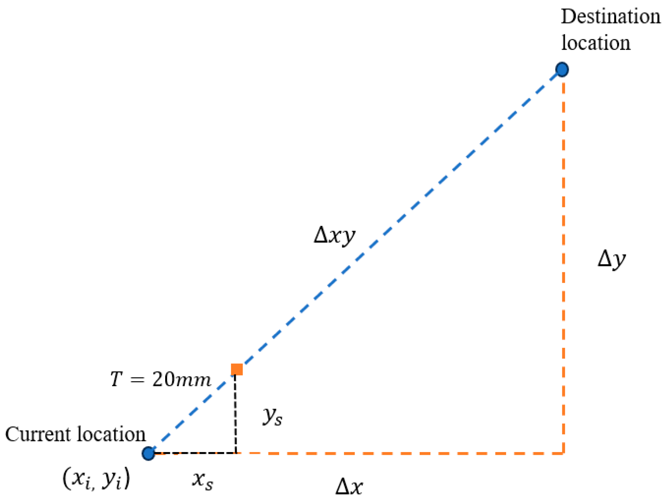
The direct distance between the current position and the final destination position (refer to
Figure 8),
, is calculated.
is based on the difference in x distance,
, and the difference in y distance, which is
, so that
.
- (iii)
If , the robot is considered to have reached the target, otherwise (i.e., if ) the robot receiver has not reached the destination yet and moves to a new position by moving and in the x and the y directions, respectively. Here and . As discussed previously, T is the step size (which is 20 mm for our experiments). It should be noted that
if , the robot moves to the right;
if , the robot moves to the left;
if , the robot moves up;
if , the robot moves down.
Once arriving at the new position, steps (i)–(iii) are reiterated until the robot arrives at its destination.
6.2. Algorithm 2
This algorithm is based on the spring relaxation [
30] or artificial potential field [
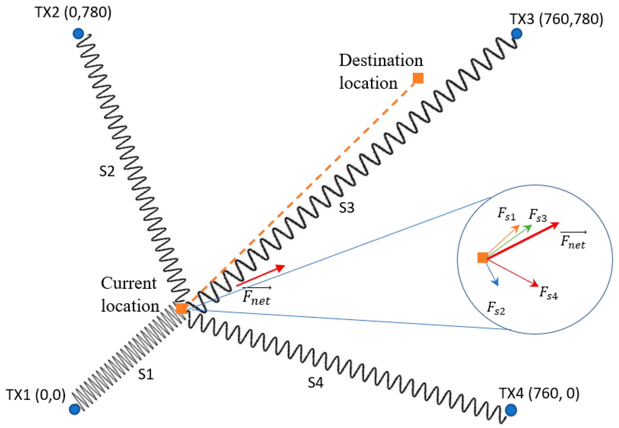
33] techniques. In this section, we explain the algorithm using the concept of spring relaxation which uses fictitious springs and Hooke’s law to guide the robot to its destination/s.
Figure 9 illustrates the concept of spring relaxation.
The location of the luminaires is the anchor to which the one end of each fictitious spring is connected. The other ends are connected to the robot. The distance between the target destination and each anchor is the natural length of each corresponding spring. Therefore, when the robot is at its destination, all the springs are relaxed (neither compressed nor stretched) and no force is acting on any of them. The goal of the algorithm is to move the robot to a position where the net force acting on the springs is zero (or below a certain threshold).
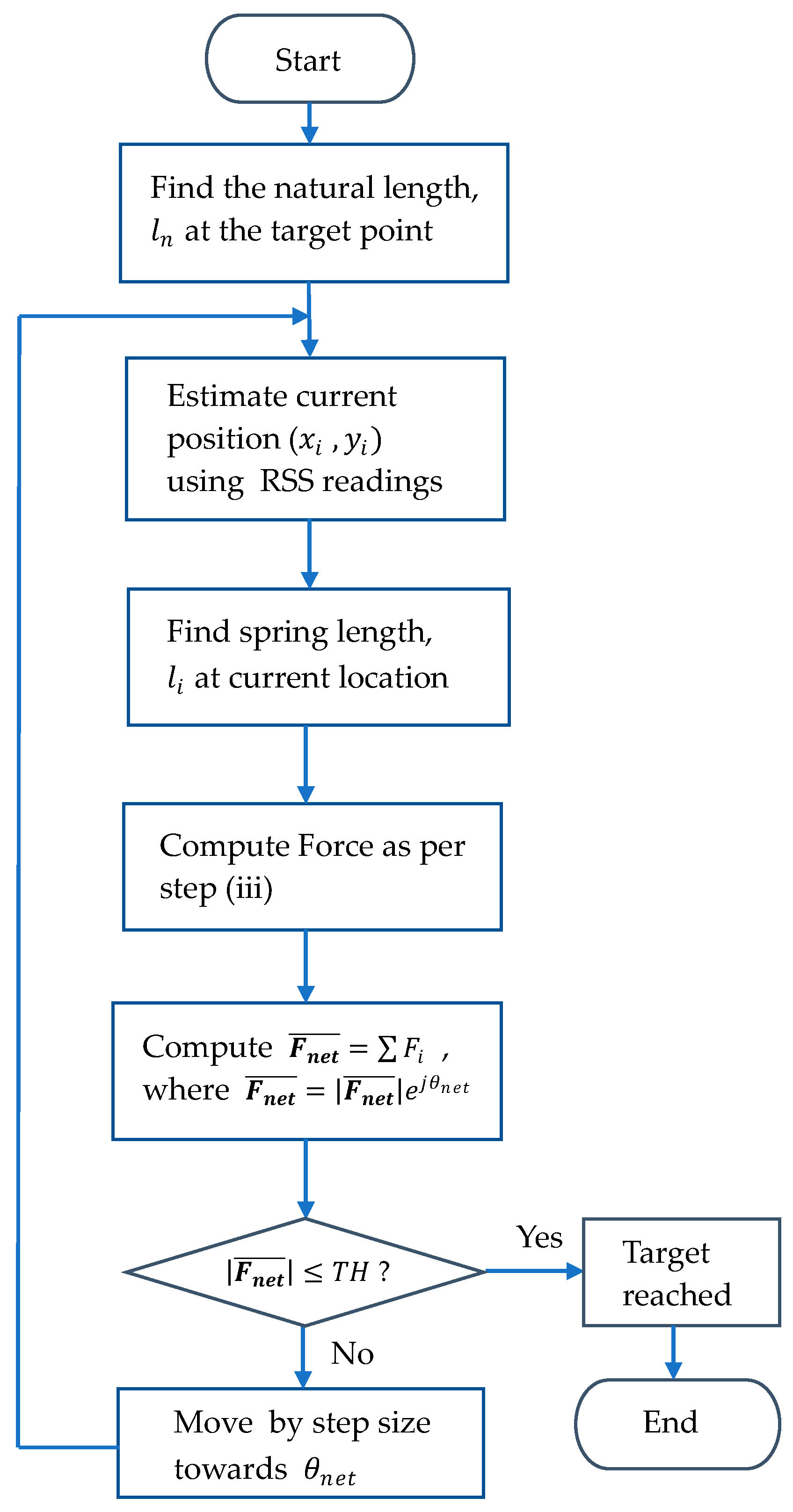
Figure 10 shows the flowchart of the algorithm.
- (i)
Compute the natural length, ( for our experimental setup), of the four fictitious springs of the sensor device at the target position.
- (ii)
Take an RSS reading at the current position,
. Next, calculate the distance of the robot from each luminaire using the ranging process described in
Section 5.2 Equations (3) and (4). Each of these distances represents the current length of each spring,
(
for our experimental setup).
- (iii)
If the current location is not the destination, the springs are not in an equilibrium state (either compressed or stretched). A compressed spring experiences a push away from the anchor, whereas a stretched spring experiences a pull toward the anchor. The individual force, , exerted by each spring, is estimated as , where is the magnitude of the force and is the direction of the corresponding force.
- (iv)
Compute the net force acting on the robot as . Note that , where is the magnitude of the net force and is the direction of the net force. If the net force is smaller than or equal to a threshold (), the robot is at the target. If not (i.e., ), the robot moves toward the direction of the net force at the step size T. Steps (i)–(iv) are repeated and the robot moves until it reaches the destination.
Figure 11 shows the tasks completed by the PC to perform the navigation of the end-effector from the starting point to the next location.
7. Experimental Results
Figure 12,
Figure 13 and
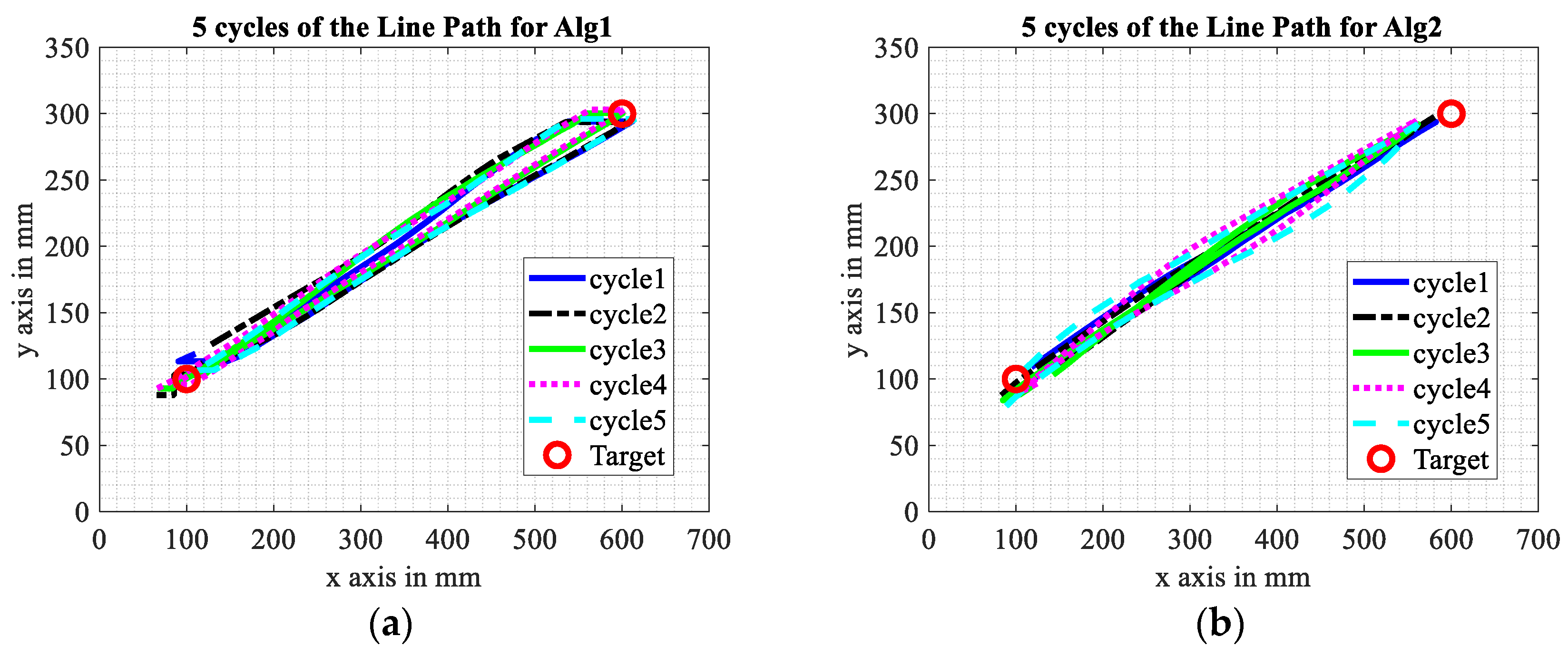
Figure 14 show how the CNC end-effector traverses through various paths. Each path is repeated five times. The actual location of the end-effector can be determined to an accuracy of 0.1 mm since the CNC tracks and records its position. Please note that this information is only used as the ground truth and is not used to control the end-effector which is solely driven by one of the algorithms based on the acquired RSS. As can be seen, VLP-driven algorithms can control the robot reasonably accurately (accuracy statistics are discussed later). However, it is also clear that for all patterns, the robot does deviate from the ideal straight-line path. This is because the VLP-based position estimate using RSS data has some error. Due to this and the discrete nature of the robot’s movement (step size of 20 mm), it does not reach the “target” points precisely. For every pattern, each path traversed is also slightly different regardless of the algorithm utilized. Therefore, the robot and the VLP-based control system, in its current state, does not have the precision or repeatability to be used for applications like assembly of electronic devices [
34].
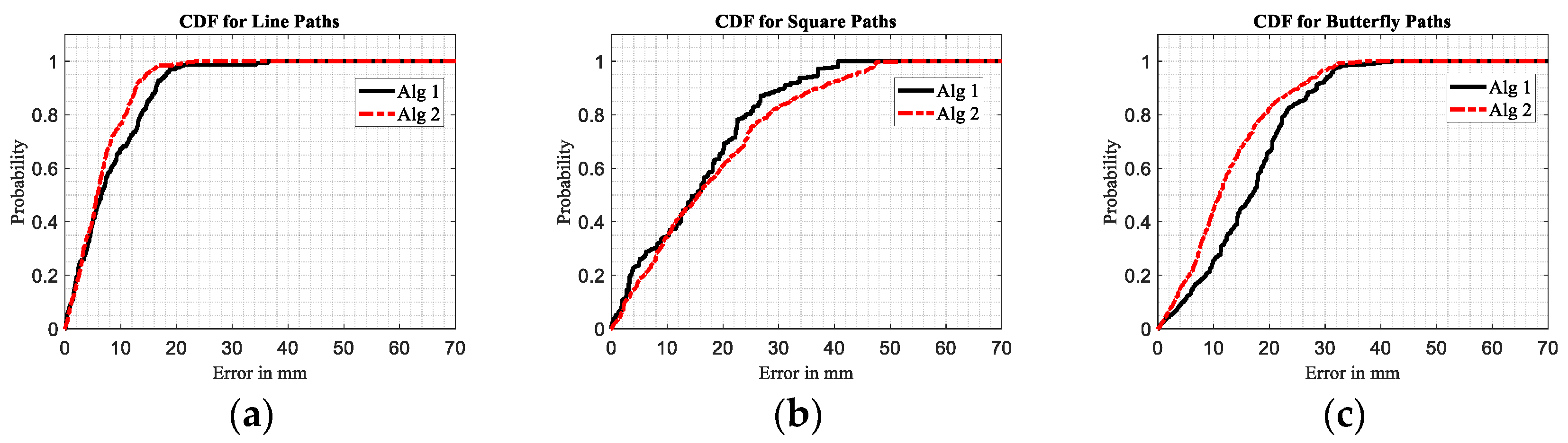
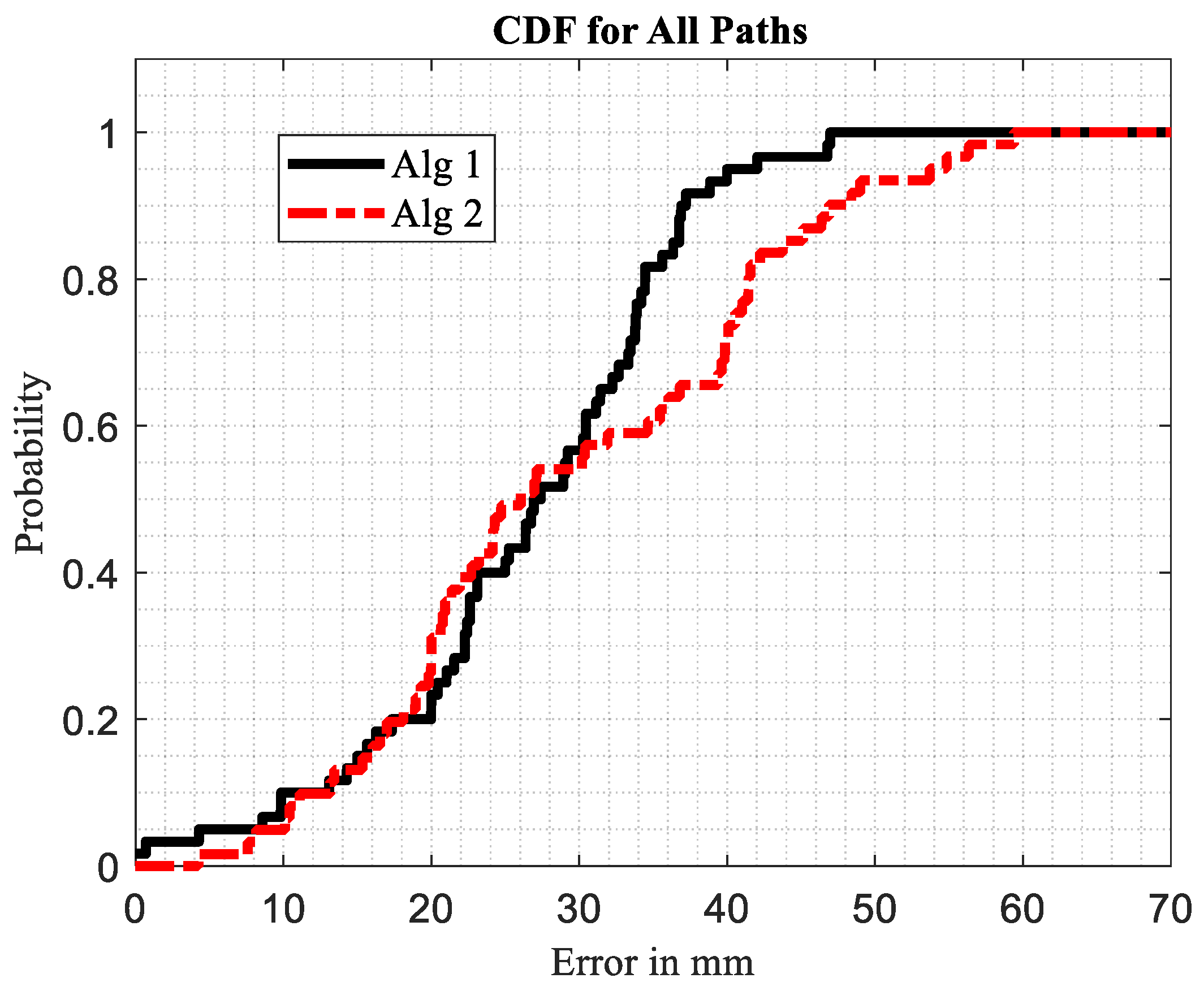
Figure 15 shows the cumulative distribution function (CDF) of the errors for each path. The error is computed as the amount of the deviation of the robot’s locations from an ideal straight line.
Figure 16 shows the CDF of the errors in reaching the target (measured as the difference between the destination point and where the robot stopped) for all the paths. The median and 90-percentile errors are shown in
Table 2. It should be noted that the errors in reaching the target can be reduced by lowering the step size (e.g., 27.16 mm to 15.23 mm for Alg1 when the step size is changed from 20 mm to 5 mm). But that comes at the cost of higher computational cost and increased time.
8. Conclusions and Future Works
This work presented the control of a cartesian robot, a 2D CNC machine, capable of precise positioning along the X and Y axes using only a PD-based VLP system. Two algorithms were developed to control the position of the robot in real time. Both algorithms show promising accuracy. Algorithm 1 performed better for the “square path”, achieving a 15.15 mm median localization error. Algorithm 2 performed better for the “line path” and the “butterfly path”, achieving median localization errors of 5.86 mm and 11.1 mm, respectively. Given the accurate performance of the system, further investigation is warranted. Also, further investigation needs to be carried out before an algorithm can be conclusively recommended. There are several other limitations that can be addressed in the future.
The locations of the luminaires of the VLP have not been optimized. Future works can explore the optimization of the layout of the VLP system. However, it should be noted that as part of real-world implementation, the location of the luminaire may be dictated by the need for illumination.
The Lambertian model was simplified under the assumption that the PD and the luminaires are parallel. If the receiver tilts, the localization estimate is affected. However, there are models [
35] that address this issue and can thus be adopted. A simple gimbal can also ensure that the receiver maintains its orientation.
Pose comprises of location and orientation. For this work, the location was determined via VLP. The orientation was determined via a CNC. Therefore, developing a new receiver capable of VLP-based orientation estimation will enable more sophisticated control strategies. Bernades et al. [
36] proposed a multi-PD based system for estimating the orientation of the receiver for an infrared (IR)-based positioning system. A similar approach can be applied for estimating the complete pose (both location and orientation) of the receiver. Incorporating orientation information into the algorithm and conducting new benchmarking experiments will open new avenues for investigation. Obstacle avoidance and path planning can also be investigated in the future. But this will require utilizing other sensors alongside PD.
Author Contributions
Conceptualization, M.-T.C. and F.A.; methodology, M.-T.C. and F.A.; software, M.-T.C., F.A. and M.L.; validation, F.A.; formal analysis, M.-T.C. and F.A.; investigation, M.-T.C.; resources, F.K.N. and F.A.; data curation, M.-T.C., F.A. and M.L.; writing—original draft preparation, M.-T.C.; writing—review and editing, F.A. and F.K.N.; visualization, M.-T.C. and F.A.; supervision, F.A., M.L. and G.S.G.; project administration, M.-T.C.; funding acquisition, F.A. All authors have read and agreed to the published version of the manuscript.
Funding
This research received no external funding.
Data Availability Statement
The data presented in this work are available upon request from other researchers and authors.
Acknowledgments
The authors wish to thank Alex Xu for his help in setting up the VLP experiment and data collection.
Conflicts of Interest
The authors declare no conflicts of interest.
References
- Kala, R. Autonomous Mobile Robots: Planning, Navigation and Simulation; Academic Press: Cambridge, MA, USA, 2023. [Google Scholar]
- Rubio, F.; Valero, F.; Llopis-Albert, C. A review of mobile robots: Concepts, methods, theoretical framework, and applications. Int. J. Adv. Robot. Syst. 2019, 16, 1729881419839596. [Google Scholar] [CrossRef]
- Peta, K.; Wlodarczyk, J.; Maniak, M. Analysis of trajectory and motion parameters of an industrial robot cooperating with a numerically controlled machine tools. J. Manuf. Process. 2023, 101, 1332–1342. [Google Scholar] [CrossRef]
- Alatise, M.B.; Hancke, G.P. A review on challenges of autonomous mobile robot and sensor fusion methods. IEEE Access 2020, 8, 39830–39846. [Google Scholar] [CrossRef]
- Guan, W.; Chen, S.; Wen, S.; Tan, Z.; Song, H.; Hou, W. High-accuracy robot indoor localization scheme based on robot operating system using visible light positioning. IEEE Photon. J. 2020, 12, 1–16. [Google Scholar] [CrossRef]
- Hayward, S.; van Lopik, K.; Hinde, C.; West, A. A survey of indoor location technologies, techniques and applications in industry. Internet Things 2022, 20, 100608. [Google Scholar] [CrossRef]
- Siegwart, R.; Nourbakhsh, I.R.; Scaramuzza, D. Introduction to Autonomous Mobile Robots; MIT Press: Cambridge, MA, USA, 2011. [Google Scholar]
- Khanh, T.T.; Nguyen, V.; Pham, X.-Q.; Huh, E.-N. Wi-Fi indoor positioning and navigation: A cloudlet-based cloud computing approach. Hum.-Centric Comput. Inf. Sci. 2020, 10, 32. [Google Scholar] [CrossRef]
- Essa, E.; Abdullah, B.A.; Wahba, A. Improve performance of indoor positioning system using ble. In Proceedings of the 2019 14th International Conference on Computer Engineering and Systems (ICCES), Cairo, Egypt, 17 December 2019; IEEE: Piscataway, NJ, USA, 2019; pp. 234–237. [Google Scholar]
- Cheng, Y.; Zhou, T. UWB indoor positioning algorithm based on TDOA technology. In Proceedings of the 2019 10th International Conference on Information Technology in Medicine and Education (ITME), Qingdao, China, 23–25 August 2019; IEEE: Piscataway, NJ, USA, 2019; pp. 777–782. [Google Scholar]
- Sasikala, M.; Athena, J.; Rini, A.S. Received Signal Strength based Indoor Positioning with RFID. In Proceedings of the 2021 IEEE International Conference on RFID Technology and Applications (RFID-TA), Delhi, India, 6–8 October 2021; IEEE: Piscataway, NJ, USA, 2021; pp. 260–263. [Google Scholar]
- Jung, J.; Lee, S.-M.; Myung, H. Indoor mobile robot localization and mapping based on ambient magnetic fields and aiding radio sources. IEEE Trans. Instrum. Meas. 2014, 64, 1922–1934. [Google Scholar] [CrossRef]
- Matheus, L.E.M.; Vieira, A.B.; Vieira, L.F.; Vieira, M.A.; Gnawali, O. Visible light communication: Concepts, applications and challenges. IEEE Commun. Surv. Tutor. 2019, 21, 3204–3237. [Google Scholar] [CrossRef]
- Zhuang, Y.; Hua, L.; Qi, L.; Yang, J.; Cao, P.; Cao, Y.; Wu, Y.; Thompson, J.; Haas, H. A survey of positioning systems using visible LED lights. IEEE Commun. Surv. Tutor. 2018, 20, 1963–1988. [Google Scholar] [CrossRef]
- Bastiaens, S.; Raes, W.; Stevens, N.; Martens, L.; Joseph, W.; Plets, D. Impact of a photodiode’s angular characteristics on RSS-based VLP accuracy. IEEE Access 2020, 8, 83116–83130. [Google Scholar] [CrossRef]
- Amsters, R.; Demeester, E.; Stevens, N.; Slaets, P. In-depth analysis of unmodulated visible light positioning using the iterated extended kalman filter. Sensors 2019, 19, 5198. [Google Scholar] [CrossRef] [PubMed]
- Afzalan, M.; Jazizadeh, F. Indoor positioning based on visible light communication: A performance-based survey of real-world prototypes. ACM Comput. Surv. (CSUR) 2019, 52, 1–36. [Google Scholar] [CrossRef]
- Glass, T.; Alam, F.; Legg, M.; Noble, F. Autonomous fingerprinting and large experimental data set for visible light positioning. Sensors 2021, 21, 3256. [Google Scholar] [CrossRef] [PubMed]
- Rahman, A.M.; Li, T.; Wang, Y. Recent advances in indoor localization via visible lights: A survey. Sensors 2020, 20, 1382. [Google Scholar] [CrossRef] [PubMed]
- Tuan-Kiet, T.; Huynh, H.-T.; Nguyen, D.-P.; Dinh-Dung, L.; Thi-Hong, T.; Nakaashima, Y. Demonstration of a visible light receiver using rolling-shutter smartphone camera. In Proceedings of the 2018 International Conference on Advanced Technologies for Communications (ATC), Ho Chi Minh City, Vietnam, 18–20 October 2018; IEEE: Piscataway, NJ, USA, 2018; pp. 214–219. [Google Scholar]
- Hamagami, R.; Ebihara, T.; Wakatsuki, N.; Maeda, Y.; Mizutani, K. Rolling-shutter sensor-based visible light communication with cross-screen filter: Communication and positioning system using a commercial camera. In Proceedings of the 2021 IEEE 10th Global Conference on Consumer Electronics (GCCE), Kyoto, Japan, 12–15 October 2021; IEEE: Piscataway, NJ, USA, 2021; pp. 386–390. [Google Scholar]
- Li, X.; Hassan, N.B.; Burton, A.; Ghassemlooy, Z.; Zvanovec, S.; Perez-Jimenez, R. A simplified model for the rolling shutter based camera in optical camera communications. In Proceedings of the 2019 15th International Conference on Telecommunications (ConTEL), Graz, Austria, 3–5 July 2019; IEEE: Piscataway, NJ, USA, 2019; pp. 1–5. [Google Scholar]
- Rátosi, M.; Simon, G. Real-time localization and tracking using visible light communication. In Proceedings of the 2018 International Conference on Indoor Positioning and Indoor Navigation (IPIN), Nantes, France, 24–27 September 2018; IEEE: Piscataway, NJ, USA, 2018; pp. 1–8. [Google Scholar]
- Li, D.; Wei, Z.; Yang, G.; Yang, Y.; Li, J.; Yu, M.; Lin, P.; Lin, J.; Chen, S.; Lu, M. Deep learning-based robust visible light positioning for high-speed vehicles. Photonics 2022, 9, 632. [Google Scholar] [CrossRef]
- Hua, L.; Zhuang, Y.; Li, Y.; Wang, Q.; Zhou, B.; Qi, L.; Yang, J.; Cao, Y.; Haas, H. FusionVLP: The fusion of photodiode and camera for visible light positioning. IEEE Trans. Veh. Technol. 2021, 70, 11796–11811. [Google Scholar] [CrossRef]
- Zhuang, Y.; Wang, Q.; Shi, M.; Cao, P.; Qi, L.; Yang, J. Low-power centimeter-level localization for indoor mobile robots based on ensemble Kalman smoother using received signal strength. IEEE Internet Things J. 2019, 6, 6513–6522. [Google Scholar] [CrossRef]
- Guan, W.; Huang, L.; Wen, S.; Yan, Z.; Liang, W.; Yang, C.; Liu, Z. Robot localization and navigation using visible light positioning and SLAM fusion. J. Light. Technol. 2021, 39, 7040–7051. [Google Scholar] [CrossRef]
- Guan, W.; Huang, L.; Hussain, B.; Yue, C.P. Robust robotic localization using visible light positioning and inertial fusion. IEEE Sens. J. 2021, 22, 4882–4892. [Google Scholar] [CrossRef]
- Liang, Q.; Lin, J.; Liu, M. Towards robust visible light positioning under LED shortage by visual-inertial fusion. In Proceedings of the 2019 International Conference on Indoor Positioning and Indoor Navigation (IPIN), Pisa, Italy, 30 September–3 October 2019; IEEE: Piscataway, NJ, USA, 2019; pp. 1–8. [Google Scholar]
- Alam, F.; Faulkner, N.; Legg, M.; Demidenko, S. Indoor visible light positioning using spring-relaxation technique in real-world setting. IEEE Access 2019, 7, 91347–91359. [Google Scholar] [CrossRef]
- Alam, F.; Chew, M.T.; Wenge, T.; Gupta, G.S. An accurate visible light positioning system using regenerated fingerprint database based on calibrated propagation model. IEEE Trans. Instrum. Meas. 2018, 68, 2714–2723. [Google Scholar] [CrossRef]
- Alam, F.; Parr, B.; Mander, S. Visible light positioning based on calibrated propagation model. IEEE Sens. Lett. 2018, 3, 1–4. [Google Scholar] [CrossRef]
- Xinyu, W.; Xiaojuan, L.; Yong, G.; Jiadong, S.; Rui, W. Bidirectional potential guided rrt* for motion planning. IEEE Access 2019, 7, 95046–95057. [Google Scholar] [CrossRef]
- Metzner, M.; Leurer, S.; Handwerker, A.; Karlidag, E.; Blank, A.; Hefner, F.; Franke, J. High-precision assembly of electronic devices with lightweight robots through sensor-guided insertion. Procedia CIRP 2021, 97, 337–341. [Google Scholar] [CrossRef]
- Shen, S.; Li, S.; Steendam, H. Simultaneous position and orientation estimation for visible light systems with multiple LEDs and multiple PDs. IEEE J. Sel. Areas Commun. 2020, 38, 1866–1879. [Google Scholar] [CrossRef]
- Bernardes, E.; Viollet, S.; Raharijaona, T. A three-photo-detector optical sensor accurately localizes a mobile robot indoors by using two infrared light-emitting diodes. IEEE Access 2020, 8, 87490–87503. [Google Scholar] [CrossRef]
Figure 1.
VLP system test rig.
Figure 1.
VLP system test rig.
Figure 2.
Modulator driver circuit.
Figure 2.
Modulator driver circuit.
Figure 3.
Key concept of the VLP system. RSS is extracted from the received signal using FFT. A representative RSS from four visible luminaires is shown at the receiver at a particular location. The measured RSS is used for model calibration during the offline stage and for ranging and localization during the live stage.
Figure 4.
Parameters of the Lambertian propagation model.
Figure 4.
Parameters of the Lambertian propagation model.
Figure 5.
The location of the luminaires and the 29 measurement locations for offline parameter calibration of the Lambertian propagation model.
Figure 5.
The location of the luminaires and the 29 measurement locations for offline parameter calibration of the Lambertian propagation model.
Figure 6.
Calibration of the Lambertian propagation models for the four luminaires.
Figure 6.
Calibration of the Lambertian propagation models for the four luminaires.
Figure 7.
Flowchart of Algorithm 1. Please see
Figure 8 for details on ∆
x, ∆
y, and ∆
xy.
Figure 7.
Flowchart of Algorithm 1. Please see
Figure 8 for details on ∆
x, ∆
y, and ∆
xy.
Figure 8.
Robot travels in a planned straight path from the current location to the destination location.
Figure 8.
Robot travels in a planned straight path from the current location to the destination location.
Figure 9.
Spring relaxation technique to guide CNC robot sensor to travel from current location to the destination location; it shows the various forces exerted by each spring, to , and the resultant net force, .
Figure 9.
Spring relaxation technique to guide CNC robot sensor to travel from current location to the destination location; it shows the various forces exerted by each spring, to , and the resultant net force, .
Figure 10.
Flow chart of Algorithm 2.
Figure 10.
Flow chart of Algorithm 2.
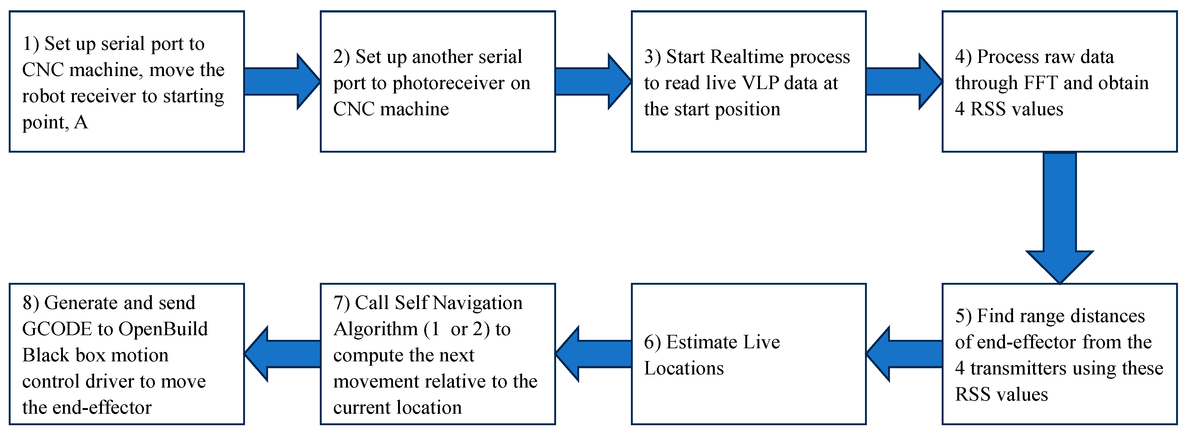
Figure 11.
The tasks completed by the PC to control the movement of the CNC end-effector while guided by one of the two algorithms running on live RSS data. Steps 3 to 8 are iterated until the end-effector reaches the destination (when the loop ends after step 6).
Figure 11.
The tasks completed by the PC to control the movement of the CNC end-effector while guided by one of the two algorithms running on live RSS data. Steps 3 to 8 are iterated until the end-effector reaches the destination (when the loop ends after step 6).
Figure 12.
“Line Path” travelled by the robot. The robot is moving from point A (100, 100) to point B (600, 300) and then returning back to A. The diagrams ((a,b) for algorithms 1 and 2, respectively) show five iterations of the path.
Figure 12.
“Line Path” travelled by the robot. The robot is moving from point A (100, 100) to point B (600, 300) and then returning back to A. The diagrams ((a,b) for algorithms 1 and 2, respectively) show five iterations of the path.
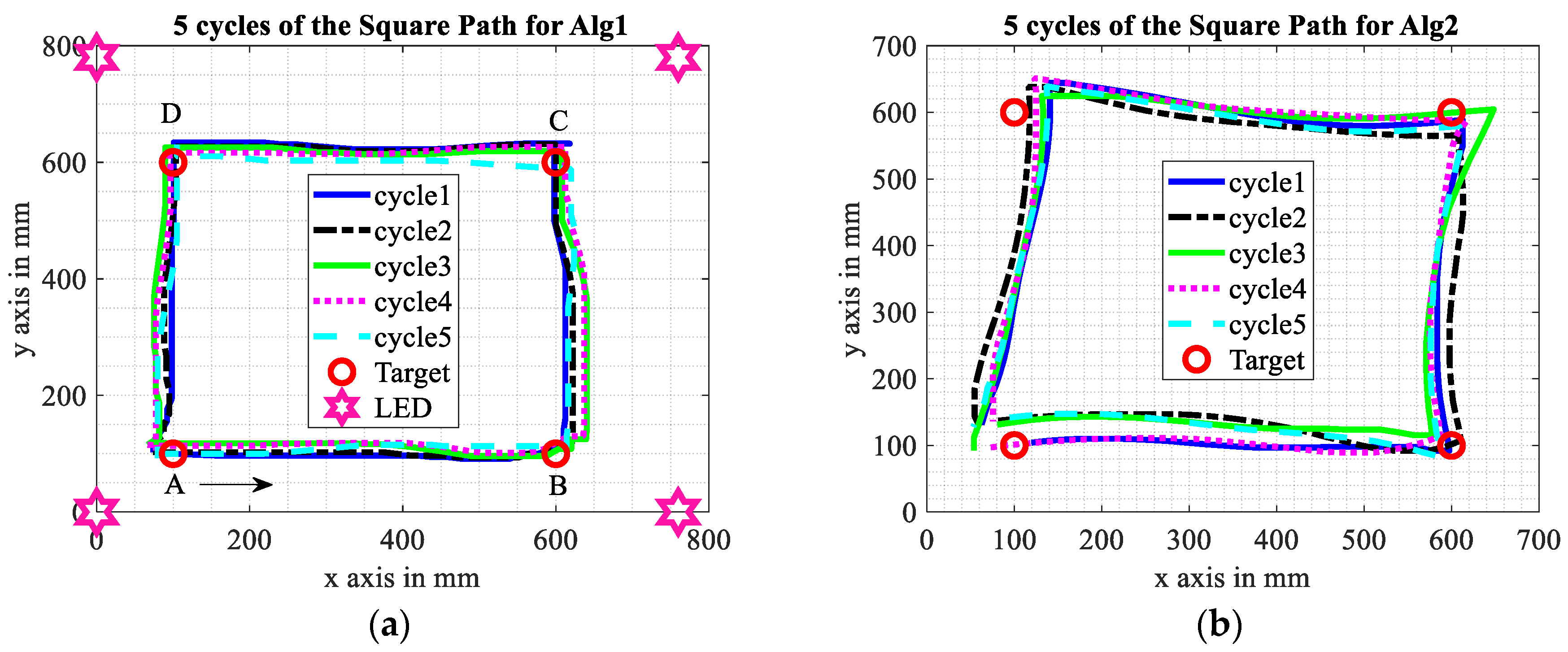
Figure 13.
“Square Path” travelled by the robot. The robot is moving from point A (100, 100) to point B (600, 100) to point C (600, 600) to point D (100, 600) to point A. The diagrams ((a,b) for Algorithms 1 and 2, respectively) show five consecutive iterations of the path.
Figure 13.
“Square Path” travelled by the robot. The robot is moving from point A (100, 100) to point B (600, 100) to point C (600, 600) to point D (100, 600) to point A. The diagrams ((a,b) for Algorithms 1 and 2, respectively) show five consecutive iterations of the path.
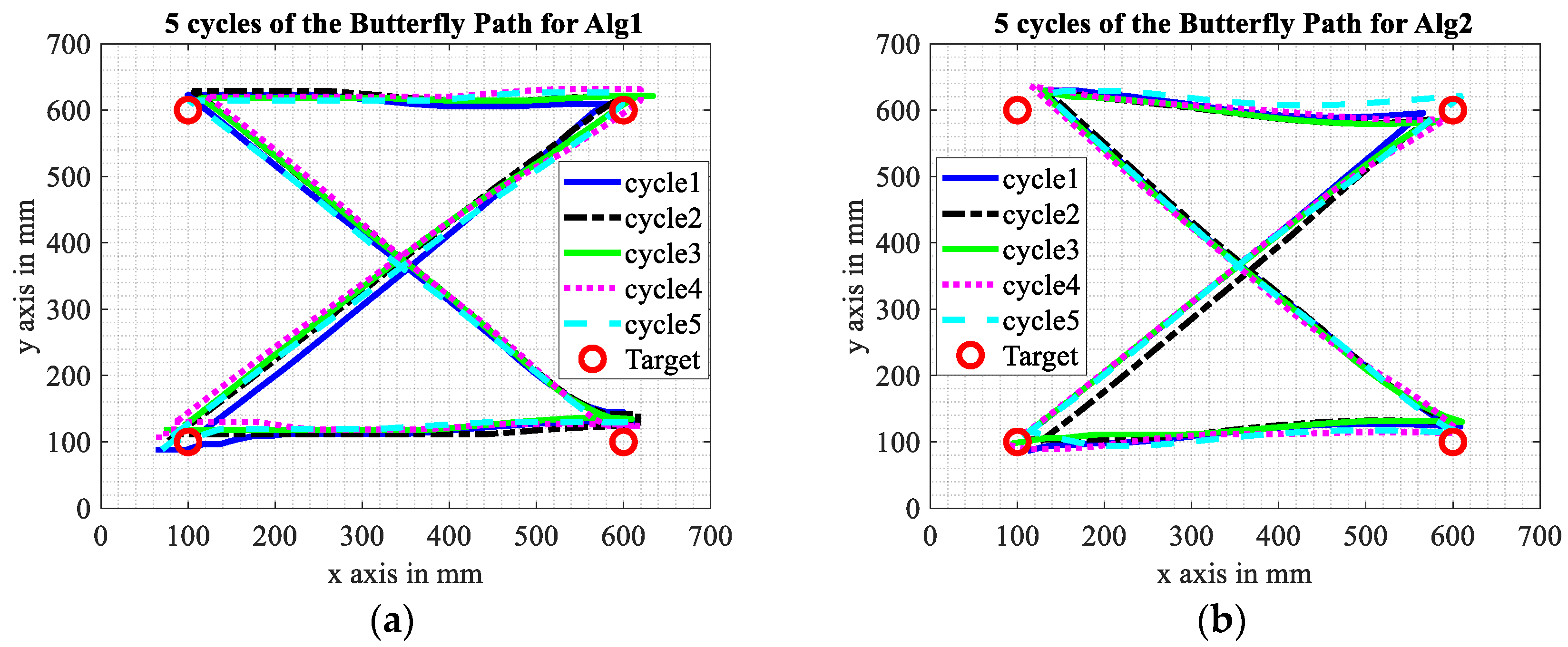
Figure 14.
“Butterfly Path” travelled by the robot. The robot is moving from point A (100, 100) to point C (600, 600); then point C to point D (100, 600); then point D to B (600, 100) and then point B to A. The diagrams ((a,b) for Algorithms 1 and 2, respectively) show five iterations of the path.
Figure 14.
“Butterfly Path” travelled by the robot. The robot is moving from point A (100, 100) to point C (600, 600); then point C to point D (100, 600); then point D to B (600, 100) and then point B to A. The diagrams ((a,b) for Algorithms 1 and 2, respectively) show five iterations of the path.
Figure 15.
CDF showing the accuracy of both algorithms for (a) Line Paths, (b) Square Paths, and (c) Butterfly Paths.
Figure 15.
CDF showing the accuracy of both algorithms for (a) Line Paths, (b) Square Paths, and (c) Butterfly Paths.
Figure 16.
Comparing “Target” positions accuracy.
Figure 16.
Comparing “Target” positions accuracy.
Table 1.
Estimated Lambertian order of the luminaires.
Table 1.
Estimated Lambertian order of the luminaires.
| Luminaire | Lambertian Order (mi) |
|---|
| 1 | 4.60 |
| 2 | 3.98 |
| 3 | 3.20 |
| 4 | 3.58 |
Table 2.
Accuracy statistics for both algorithms for various scenarios.
Table 2.
Accuracy statistics for both algorithms for various scenarios.
| Scenario | Median Error (mm) | 90-Percentile Error (mm) |
|---|
| Algorithm 1 | Algorithm 2 | Algorithm 1 | Algorithm 2 |
|---|
| Line Path | 8.02 | 5.86 | 16.34 | 12.71 |
| Square Path | 15.15 | 15.51 | 30.99 | 37.59 |
| Butterfly Path | 16.81 | 11.1 | 28.48 | 25.19 |
| Destination Points | 27.16 | 26.05 | 37.04 | 47.48 |
| Disclaimer/Publisher’s Note: The statements, opinions and data contained in all publications are solely those of the individual author(s) and contributor(s) and not of MDPI and/or the editor(s). MDPI and/or the editor(s) disclaim responsibility for any injury to people or property resulting from any ideas, methods, instructions or products referred to in the content. |
© 2024 by the authors. Licensee MDPI, Basel, Switzerland. This article is an open access article distributed under the terms and conditions of the Creative Commons Attribution (CC BY) license (https://creativecommons.org/licenses/by/4.0/).


