Research on a Resource Modeling and Power Prediction Method Based on Virtual Aggregation

Abstract

Distributed resources at a grid’s end cannot upload operational power data to local centers due to data transmission and privacy issues. This leaves the centers with incomplete information, thus impacting decision making. This paper presents a virtual aggregation-based model for such scenarios. We define four virtual aggregate types based on resource response characteristics. Using characteristic coefficients, we identify these aggregates’ categories and proportions from bus power. To address blind source separation in single-channel power signals, we apply the Ensemble Empirical Mode Decomposition-Fast Independent Component Analysis (EEMD-FastICA) method. This helps extract and analyze bus power, thereby deriving power curves for different aggregates. Moreover, we use a graph convolutional network to explore how factors like date, time, weather, and pricing intertwine with aggregate power. We develop a predictive model with an advanced SpatioTemporal Graph Convolutional Network (STGCN), thus facilitating proactive power forecasting for virtual aggregates. Case studies show our method’s efficacy in extracting power curves under limited information, with the STGCN ensuring accurate, forward-looking predictions.

1. Introduction

Within the aim of carbon neutrality, there are three major trends in China’s energy system: firstly, there is the electrification of the energy system [1], which means that, by 2050, the proportion of primary energy to electricity conversion and the proportion of electricity to terminal energy consumption are expected to increase to 80% and 60%, respectively; secondly, the low-carbon power system is expected to increase the proportion of nonfossil energy generation from the current 33% to 84–90% by 2050 [2]; and thirdly, the decentralization of energy and power systems is being sought. The mode of energy development and utilization will shift from centralized to distributed, and the form of energy systems will undergo profound changes [3]. With the advancement of energy transformation, the types and quantities of distributed resources in regional power grids have shown explosive growth, and this mainly includes load-side distributed resources, which are represented by electric vehicles [4], temperature-controlled loads [5], and energy storage [6]. Conversely, power-side distributed resources are represented by wind and photovoltaic power. Compared with traditional adjustable and controllable resources, such as large water/thermal power units, the abovementioned distributed resources have advantages such as small individual capacity, numerous quantities, huge potential, green environmental protection, and flexible economy, which are of great significance for enhancing the balance and regulation ability of regional power grids. However, due to the distributed resources being located at the end of the power grid, the dispatch control center is unable to achieve the comprehensive observation and control of massive terminal data, thereby resulting in a contradiction between scheduling requirements and the efficient matching of massive distributed resources. In addition, the privacy protection requirements of distributed resource entities bring about incomplete information, making it difficult for the scheduling control center to obtain detailed operational characteristics of certain distributed resources. Therefore, the focus of this article is on how to scientifically model the equivalence of distributed resources in the presence of incomplete information.

Currently, experts and scholars, both domestically and internationally, have conducted extensive research in this field, thereby providing valuable insights and models for our learning and reference.

(1)

The Operational Characteristics of Distributed Resources

Scholars, both domestically and internationally, have conducted extensive research on the operational characteristics of distributed resources. Ref. [7] proposed a multimodel weighted parameter identification method for modeling user electricity elasticity using the weighted average of four linear models to establish a comprehensive model for user elasticity. However, the simulation did not consider the mutual elasticity of users at different time periods. Ref. [8] established an objective function for market operation revenue based on the user’s profit function, and they also derived the optimal incentive price. However, the key parameters in the user’s profit function involve privacy and public willingness, making it relatively difficult to obtain. The household energy management system proposed in [9] is based on an energy monitoring module, and it participates in demand response and provides electrical level energy optimization.

(2)

The Extraction of Load Characteristic Parameters

In terms of load characteristic parameter extraction, the extraction methods mainly include time domain and frequency domain, and the feature extraction objects include active power, reactive power, voltage, current [10,11], etc. Ref. [12] extracted six parameters, including load rate, maximum utilization hours, daily peak valley difference rate, and peak/valley/average load rate, as well as the characteristic indicators of load morphology for the demand-side load of the Shanghai power grid. Ref. [13] extracted characteristic parameters such as maximum load occurrence time to achieve daily load curve clustering. Ref. [14] proposed parameters such as the load regulation coefficient, jump rate, and load stability to characterize the adjustable characteristics of loads. Ref. [15] adopted a method that combines time information and active power to achieve load separation identification; refs. [16,17,18] extracted harmonic signals and low-power features. In the field of noninvasive identifications of household electrical loads, researchers have proposed extraction algorithms for active power fluctuation characteristics and the incremental characteristics of loads [19].

(3)

Load Identification

At present, most of the research on load feature extraction methods has mainly focused on the fields of electricity load classification in different industries and the noninvasive identification of household loads, but there has been relatively little research on resource aggregation feature extraction methods for the characterization of demand response regulation characteristics. In terms of load identification, ref. [15] proposed an industry-typical feature matrix, as well as obtained an online correction method for the various types of load composition ratios of daily load curves based on the calculation of feature matrices and membership degrees. Ref. [16] proposed a load identification method based on the fuzzy clustering theory for the feature extraction of adjustable/interruptible loads.

(4)

Dynamic Electricity Pricing Management

Dynamic electricity price management is one of the main management methods that is based on distribution system operators (DSOs), and electricity price signals are an important way through which to motivate distributed energy resources (DERs) in order to participate in power grid regulation. By replacing direct control commands with electricity price signals, DERs can actively participate in the management of power grids. Dynamic electricity price management is often used in distribution network congestion management, and the electricity price mechanism that motivates DERs involves dynamic tariff (DT) and the distribution local marginal price (DLMP) [20]. Ref. [21] proved that the strategy of DSOs in pursuing the optimal DLMP is consistent with the strategy of electric vehicle aggregators pursuing the lowest charging cost, thereby indicating that the DLMP is an effective distribution network congestion management method. Ref. [22] incorporated the cost of reactive power regulation in distribution networks, the cost of insufficient charging capacities for electric vehicles, and the cost of distributed generation into the objective functions of the DLMP; in addition, they, respectively, obtained active and reactive DLMPs [23]. Therefore, the power prediction of resource aggregates is greatly influenced by electricity prices. When seeking to grasp the rules of the power curve of resource aggregates, comprehensive consideration should be given to electricity prices and other external factors.

In summary, in the case of incomplete information, the scientific equivalent modeling of distributed resources requires the consideration of resource feature extraction, and the accurate prediction of resource aggregation power also requires the consideration of various external factors, such as electricity prices. In order to match the work of resource aggregation with scheduling requirements and to support scheduling control centers’ observable and controllable business in massive distributed resources, this paper focuses on the key business scenario of distributed resources participating in demand response adjustment, as well as proposes a virtual aggregation-based resource aggregation modeling and power prediction method for use in incomplete information conditions. The main contributions of this article are as follows:

(1)

Based on demand response businesses, this article summarizes the regulatory characteristics of distributed resources that participate in demand response, as well as performs a virtual aggregation of distributed resources and defines four types of virtual aggregates;

(2)

This article designs algorithms to recognize and extract the power of each virtual polymer, as defined earlier, and this is conducted only from bus power in scenarios with incomplete information;

(3)

Based on the power curve of virtual aggregates, this article delves into the various environmental and electricity price factors that affect the operation power of virtual aggregates, constructs an artificial intelligence virtual aggregate power prediction model, and achieves advanced predictions of virtual aggregate power;

(4)

The numerical analysis shows the effectiveness and superiority of the method proposed in this article, which can help dispatch control centers grasp the operating power of distributed resource aggregates in scenarios with incomplete information. This method also helps to provide controllable means (electricity prices) and a fitting mapping relationship between virtual aggregate power, which can provide effective decision making for dispatch control centers, such that they can carry out economic dispatches and demand responses, as well as deliver bus load power prediction businesses.

2. The Resource Aggregation Architecture and Power Prediction Model

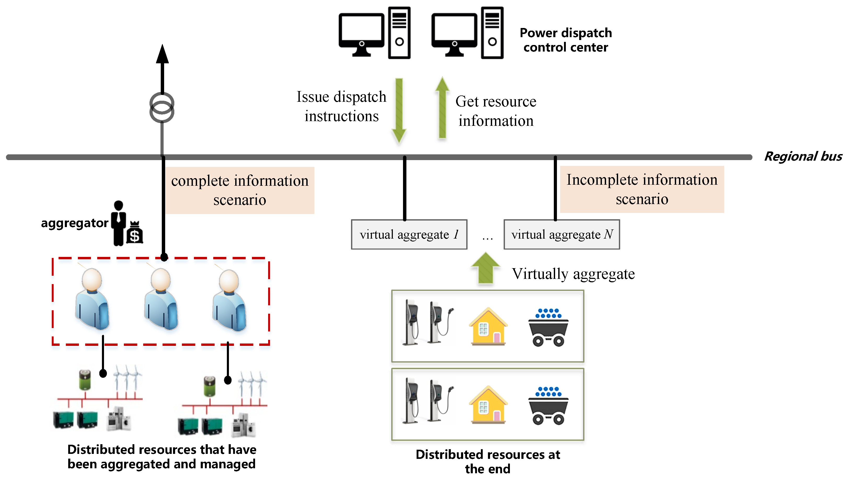
Parts of the distributed resources under regional buses are aggregated and integrated into power grid dispatch systems through third-party aggregators. Aggregators usually use certain technical means to manage distributed resources, organize resources to participate in demand response and market transactions, and support the safe operation of power grids while obtaining certain benefits. A power dispatch control center can obtain the basic operational characteristics of aggregated resources from an aggregator, including regulating capacities, regulating speeds, ramp rates, etc. In such scenarios, the historical operational data and future predictive data of resource aggregates that dispatch control centers can grasp are relatively complete, thus making it easier to support power grid dispatch decisions. However, distributed resources that are scattered at the end of electrical grids are often unable to upload their operational power data to local power dispatch control centers due to constraints in data transmission and the need for privacy protection. Consequently, dispatch control centers, as they lack visibility into the composition and operational power of terminal distributed resources, face scenarios of incomplete information, which hinder their ability to make informed dispatch decisions. In recent years, power grid dispatches have been plagued by a serious shortage of the flexible resources available to support their systems. Therefore, establishing an equivalent model of resource aggregates in scenarios with incomplete information, tapping into the regulating potential of massive distributed resources, and enriching and improving the dispatch methods of dispatch control centers is of great significance for the safe, stable, and economic operation of power grids.

In order to explore an effective method for obtaining the operational characteristics of distributed resource aggregates from bus power in scenarios with incomplete information, this paper focuses on demand response businesses and proposes a resource aggregate modeling and power prediction method based on virtual aggregation for incomplete information conditions. Different types of virtual aggregates were defined and divided based on the differences in the regulation characteristics of distributed resource execution demand responses. The operating characteristics of various virtual aggregates were extracted from bus power using single-channel blind source separation technology. The architecture of distributed resource aggregation for regional buses is shown in Figure 1.

After obtaining the power curves of various virtual aggregates, in order to seek controllable means for the power regulation of virtual aggregates and to provide auxiliary references for power grid scheduling decisions, this paper uses artificial intelligence to delve deeply into the various environmental and electricity price factors that affect the operation power of virtual aggregates. In addition, a virtual aggregate power prediction model is constructed: one that is able to provide a fitting mapping relationship between controllable means (electricity price) and virtual aggregate power, as well as one that helps to realize advanced predictions of virtual polymer power.

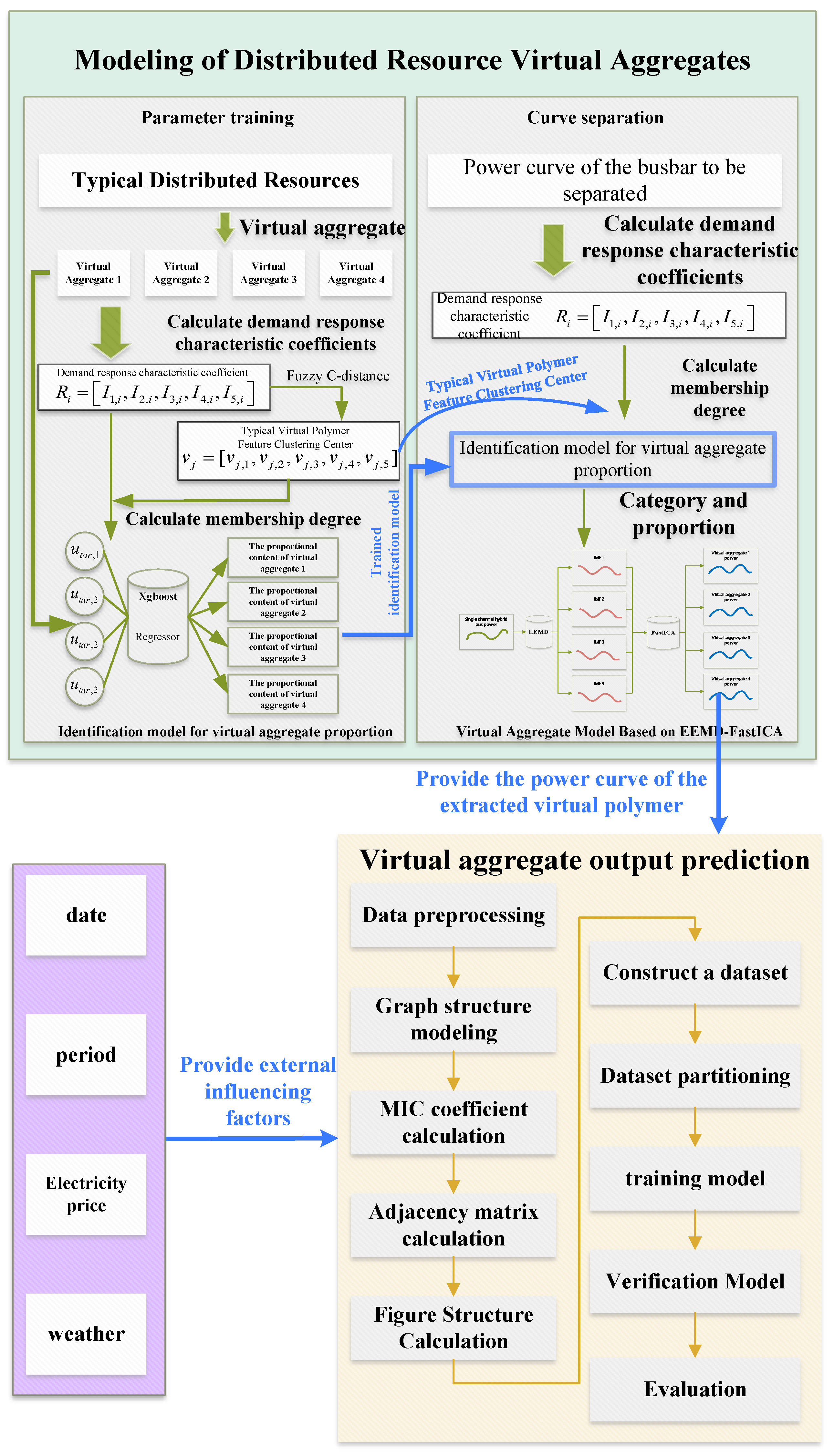
The whole process of constructing the resource aggregation modeling and a power prediction method based on the virtual aggregation that is proposed in this paper is shown in Figure 2. First, four types of virtual aggregates are defined according to the demand response characteristics of resources, and the characteristics were constructed to identify the categories and proportions of the four types of aggregates from the busbar power. The identified results are used as the number of source signals for the busbar power analysis. Secondly, to solve the problem of single-channel blind source separation, the underdetermined blind source separation method, which is based on EEMD-FastICA, was used to analyze the power of buses, and the power curves of each virtual polymer were obtained. Finally, based on an artificial intelligence method, this paper mined the nonlinear mapping relationship between the date, time period, weather, electricity price data, etc., and the behavior law of the aggregate, as well as constructed a power prediction model of virtual aggregates based on an improved STGCN. Moreover, an advanced prediction of the output of virtual aggregates so as to help dispatching control centers grasp the operation characteristics of idle distributed resources was realized.

3. Distributed Resource Virtual Aggregation Based on EEMD-FastICA

3.1. Virtual Aggregates

The distributed resources, based on their operational characteristics and the characteristics of execution demand responses, were divided into four categories: discrete adjustable resources, flexible adjustable resources, time-varying resources, and nonadjustable resources. The loads or generator sets belonging to each type of resource were subjected to virtual aggregation, thereby forming four types of virtual aggregates. These were called virtual polymers due to the fact that the resources within each polymer were not limited by industry and region, as well as because they were only used as a demand response aggregation method under incomplete information. The study of the operational and response characteristics of virtual aggregates can be used for scenarios such as bus load forecasting, demand responses, and electricity market trading decisions.

(1)

Class I virtual aggregates

Class I virtual aggregates include various distributed resources with discrete adjustable resource characteristics. Discrete adjustable resources have bidirectional adjustment ability, which can quickly adjust operating power, as well as help to approximate the instantaneous adjustment of operating power. The adjustment is flexible but the adjustment range is small, and it cannot be adjusted frequently. The response characteristic curve of discrete adjustable resources is shown in Figure 3. The black line in the figure represents the curve when the discrete adjustable resources are not adjusted, and the red line represents the power curve of the discrete adjustable resources after response adjustment.

Discrete adjustable resources have the characteristic of discrete adjustment, which manifests as follows: (1) possessing a certain adjustable space; (2) the adjustment speed is fast within limited adjustment capacity ranges; (3) and, once adjusted, it is necessary to ensure that the power is maintained for a limited time and that it cannot respond to frequent adjustment needs.

(2)

Class II virtual aggregates

Class II virtual aggregates include various distributed resources with flexible and adjustable resource characteristics. Flexible and adjustable resources have bidirectional continuous adjustment ability, flexible resource adjustment, and smooth climbing characteristics. The response characteristic curve of flexible adjustable resources is shown in Figure 4. The black line in the figure represents the curve when the flexible adjustable resources are not adjusted, and the red line represents the power curve of the flexible adjustable resources after response adjustment.

Flexible and adjustable resources have the characteristic of continuous adjustment, which manifests as follows: (1) they can be continuously adjusted within a certain capacity adjustment range; (2) they have no power stability duration requirement constraint; and (3) they can respond to adjustment needs at any time.

(3)

Class III virtual aggregates

Class III virtual aggregates include various distributed resources with time-varying resource characteristics, and they can achieve daily regulation. According to the requirements of power grid scheduling, the response speed of their power regulation can reach the millisecond level. The response speed of time-shifted resources is fast, and this is without adjusting time constraints. Time-shifted resources can change the operating period to achieve power transfer. A characteristic of it is that its total electricity energy within the day is constant, and only its operating power period changes. The response characteristic curve of time-shifted resources is shown in Figure 5. The black line in the figure represents the curve when the time-shifted resources are not adjusted, and the red line represents the power curve of the time-shifted resources after response adjustment.

Time-shifted resources have the characteristic of being adjustable, which manifests as follows: (1) being continuously adjustable within a certain capacity adjustment range; (2) able to respond to adjustment needs and can adjust speed quickly and flexibly through output transfer; (3) it can transfer the time of load electricity consumption by responding to peak and valley electricity prices; and (4) it can also ensure that the total electricity consumption remains unchanged within the days before and after load transfer.

Class I virtual aggregates and Class II virtual aggregates increase or decrease electricity consumption in specific time periods through different forms of regulation (discrete regulation, continuous regulation, etc.), while time-shifted resources transfer electricity consumption in specific time periods.

(4)

Class IV virtual aggregates.

Class IV virtual aggregates include various distributed resources with nonadjustable resource characteristics. Nonadjustable resources generally do not participate in demand responses due to their particularity, and their operating characteristics do not change under electricity prices or incentive measures. The operating curve before and after adjustment is an overlapping curve. The response characteristic curve of nonadjustable resources is shown in Figure 6. The black line represents the curve when the nonadjustable resources are not adjusted, and the red line represents the power curve of the nonadjustable resources after response adjustment.

3.2. Virtual Aggregate Identification

3.2.1. The Demand Response Characteristic Coefficient

We defined the characteristic coefficients that characterize the demand response of virtual aggregates based on the operation and response characteristics of the various virtual aggregates detailed in Section 3.1. This was performed in order to achieve the differentiation and identification of the various virtual aggregates, and we then used them to analyze and extract the operational characteristic curves of the various virtual aggregates in bus power.

This article designed the five characteristic coefficients of responsivity, response depth, response duration, response fluctuation entropy, and the response time-shift coefficient as follows:

(1)

Responsiveness

According to the above analysis, the biggest difference between the first three types of virtual polymers and the fourth type of virtual polymer is that there is no difference in the operating power curve of the fourth type of virtual polymer before and after demand response adjustment; meanwhile, the operating power curves of the other three types of virtual polymers all changed. Therefore, the responsiveness $I_1$ was designed as the first characteristic indicator, which is defined as the Pearson correlation coefficient of the power curve before and after the response of the virtual polymer.

In statistics, the Pearson correlation coefficient can represent the linear correlation strength between two variables. The Pearson correlation coefficient of the two variables was calculated using Formula (1):

$$r=\frac{\mathrm{cov}(U,V)}{{\xi }_U{\xi }_V}=\frac{E\left(UV\right)-E\left(U\right)E\left(V\right)}{\sqrt{E\left(U^2\right)-E^2\left(U\right)}\sqrt{E\left(V^2\right)-E^2\left(V\right)}},$$

(1)

where cov( ) is the covariance function; E is the mathematical expectation function; $\xi$ is the mean square deviation; and U and V are the two variables. If the absolute value of the correlation coefficient is greater than 0.5, then it is considered that the two variables have a strong correlation. According to the definition of the Pearson correlation coefficient, the correlation coefficient between the preadjustment standardized virtual polymer operating power $P_a$ and the postadjustment standardized virtual polymer operating power $P_b$ can be obtained. The mathematical expression of the response coefficient $I_1$ is as follows:

$$I_1=r\left(P_a,P_b\right).$$

(2)

(2)

Response depth

The response depth $I_2$ is defined as the maximum value of the power change during the operation of the virtual polymer before and after adjustment, and this is mathematically expressed as follows:

$$I_2=\underset{\mathrm{t}\in T}{max}\left|P_b^t-P_a^t\right|,$$

(3)

where $P_a^t$ is the standardized virtual polymer operating power adjusted for the t period; $P_b^t$ is the standardized virtual polymer operating power during the adjusted time period t; and T is the total number of time slots during the day.

(3)

Response duration

According to the response characteristics of the Class I and Class II virtual polymers, the obvious difference between the two was that Class I virtual polymers can maintain a stable operation for a period of time after response, while Class II virtual polymers can be flexibly adjusted with large changes in power. Therefore, the response duration $I_3$ was selected as the third indicator, which is mathematically expressed as follows:

$$I_3=\frac{1}{m+\epsilon }\sum T\{\left|P_b^t-P_a^t\right|\ge 0.01\},$$

(4)

where $I_3$ is the average value s of the operating power of the virtual polymer before and after adjustment during the adjustment period; m is the total number of time periods, where the difference between the two curves is greater than 0.01; $T\{\left|P_b^t-P_a^t\right|\ge 0.01\}$ is the period when the difference between the two curves is greater than 0.01; and $\epsilon ={10}^{-6}$ is a positive number with an especially small value so as to avoid the situation where the denominator is zero.

(4)

Response fluctuation entropy

Considering the fact that the fluctuation of the running power curves of various virtual polymers before and after adjustment is different, the response fluctuation entropy was thus introduced as the fourth index $I_4$. First, we introduced statistics $\mathsf{\varnothing }\left(t\right)$ as follows:

$$\mathsf{\varnothing }\left(t\right)=P_b^t/\underset{t\in T}{max}{P}_b^t.$$

(5)

The statistic $\mathsf{\varnothing }\left(t\right)$ reflects the fluctuation degree of the running power curve of the virtual polymer before and after adjustment, and its value range is [0, 1]. If the value range [0, 1] is divided into k equal parts, then the k interval can be expressed as $(\frac{k}{n},\frac{k+1}{n}]$. One can run through statistics $\mathsf{\varnothing }\left(t\right)$ at every moment of the day, and it falls into the time points of each interval. Let the moment point of the $\mathsf{\varnothing }\left(t\right)$ distributed over the k-th interval be $m_k$, then the probability that the $\mathsf{\varnothing }\left(t\right)$ is located in the interval is as follows:

$$v\left(t\right)=m_k/T.$$

(6)

Define the response fluctuation entropy $I_4$ to be the following:

$$I_4=-\sum _{k=0}^n\nu \left(k\right)ln\nu \left(k\right).$$

(7)

According to the definition of response fluctuation entropy, when the $\mathsf{\varnothing }\left(t\right)$ all fall in the same interval, the response wave entropy is the smallest and its value is equal to 0. When no $\mathsf{\varnothing }\left(t\right)$ of any period are in the same interval, the response fluctuation entropy is the largest.

(5)

Response time-shift coefficient

The response time-shift coefficient $I_5$ is defined as the ratio of the sum of the power changes in each period before and after the adjustment of the virtual polymer to the sum of the absolute value of the power changes in each period of the virtual polymer. This reflects the changes in each period of the two curves. Its mathematical expression is as follows:

$$I_5=\left[\sum _{t=0}^T\left(P_b^t-P_a^t\right)+\epsilon \right]/\left[\left|P_b^t-P_a^t\right|+\epsilon \right].$$

(8)

Considering the fact that the absolute sum of the power change before and after the regulation of the Class IV virtual polymer was zero, in order to avoid the situation where the denominator is zero, a minimal positive number $\epsilon$ was added to both the numerator and denominator of the expression; as such, $\epsilon ={10}^{-6}$ was taken. In this case, the response time-shift coefficient was 1.

For the Class III virtual polymers, the time-shift coefficient was close to 0, while for the other three virtual polymers, the time-shift coefficient was close to 1.

3.2.2. Characteristic Extraction of the Demand Response of Typical Virtual Aggregates

This section adopts the clustering method, based on the demand response feature coefficient proposed in Section 3.2.1, to extract the demand response features of various virtual aggregates.

Power curve samples of typical virtual aggregates before and after adjustment were selected to calculate the characteristic coefficient of the demand response of each sample. The vector $R_i$ of the characteristic coefficient of the demand response of the i-th power curve sample is shown as follows:

$$R_i=\left[I_{1,i},I_{2,i},I_{3,i},I_{4,i},I_{5,i}\right],$$

(9)

where $I_{1,i}, I_{2,i}, I_{3,i}, I_{4,i},$ and $I_{5,i}$ correspond to the respective five characteristic coefficients of the calculated demand response.

The clustering center of the demand response characteristic coefficients of all N samples of a typical virtual aggregate was calculated. In this paper, a fuzzy C clustering algorithm was adopted, and its basic steps are as follows:

(1)

Select the number of clustering centers.

(2)

Randomly initialize the clustering center from the sample points as follows:

$$v_j=[v_{j,1},v_{j,2},v_{j,3},v_{j,4},v_{j,5}],$$

(10)

where $v_j$ is the j-th cluster center vector.

(3)

Initialize the membership matrix, as shown in the above formula.

(4)

Update the cluster center and membership matrix, as shown in the following formula:

$$U=\left[u_{ij}\right]$$

(11)

$$u_{ij}=\frac{{\left(d_{ij}\right)}^{-1}}{{\displaystyle \sum _{l=1}^C}{\left(d_{il}\right)}^{-1}}$$

(12)

$$d_{ij}=\sum _{m=1}^5{\left({\left(R_{i,m}-v_{j,m}\right)}^2\right)}^{1/2},$$

(13)

where m is the fuzzy parameter (which is usually greater than 1).

(5)

When the change in the cluster center is less than the set threshold, or if it reaches the preset maximum number of iterations, the algorithm terminates; otherwise, the iteration continues.

In summary, the fuzzy C clustering algorithm was used to extract the demand response features of the various typical virtual aggregates by setting the number of clustering centers to $C=1$.

3.2.3. Category Identification and Proportion Determination of the Virtual Aggregates in Busbar Power

This paper modeled a hybrid bus with four types of virtual aggregates for the hybrid buses with unclear components in their distributed resources and unknown output. In this section, the demand response characteristic coefficient of the hybrid bus is calculated, and the membership degree of the hybrid bus characteristic coefficient to the four types of typical virtual aggregates is obtained by using the mapping relationship between the membership degree and the proportion of virtual aggregates. The category identification and proportion determination of the virtual aggregates are completed. The specific methods used are as follows:

Firstly, the characteristic coefficient of the demand responses of a hybrid bus was calculated according to the running power curve of the hybrid bus before and after adjustment.

Secondly, via the method detailed in Section 3.2.2, the clustering centers of each typical virtual polymer $v_1$, …, $v_4$ were ascertained, and the membership degree of the hybrid bus characteristic coefficient for the four typical virtual polymers of $u_{tar,1}$, …, $u_{tar,5}$ was calculated.

Finally, a machine learning model based on XGboost was constructed to learn the mapping relationship between the membership degree and the proportion of virtual aggregates; in addition, the category identification and proportion determination of the virtual aggregates was completed. The mapping is shown in Figure 7.

3.3. Virtual Polymer Running Power Curve Extraction

The categories and proportions of the virtual aggregates of mixed buses were obtained by means of the methods in Section 3.2. Furthermore, the operating power curves of the virtual aggregates were extracted and are detailed in this section. Since there was only one observable power curve for a mixed bus, while there were multiple operating power curves for the extracted virtual aggregates, this problem belongs to the single-channel blind source separation problem. This kind of problem is an underdetermined blind source problem, and it is impossible to directly separate the operating power curve of virtual aggregates. Therefore, this paper uses Ensemble Empirical Mode Decomposition (EEMD) to separate the single-channel mixed bus power signal into several Intrinsic Mode Function (IMF) components. Furthermore, according to the number of possible sources for a single-channel signal (i.e., the number of categories of virtual aggregates that were identified), an appropriate IMF component was selected in order to compose a new observation quantity, which was performed so as to realize the blind source separation of a single-channel mixed bus power curve signal.

3.3.1. EEMD

Ensemble Empirical Mode Decomposition (EEMD) is an extended version of Empirical Mode Decomposition (EMD). The mode aliasing problem in EMD is solved by adding a set of white noise to the raw data. The following is a basic introduction to the EEMD algorithm.

(1)

Add a series of different white noises to the original data $X\left(t\right)$ to create the multiple data sets $X_i\left(t\right)=X\left(t\right)+{\omega }_i\left(t\right)$, where ${\omega }_i\left(t\right)$ is white noise.

(2)

For each $X_i\left(t\right)$ application of EMD decomposition, carry out the decomposition into a series of IMFs.

(3)

For each IMF, the average of all noisy instances is calculated to obtain the final IMFs, i.e., the $k-th$ IMF is the average of the $k-th$ IMFs, which is obtained by decomposing all $X_i\left(t\right)$.

Here are the steps for EMD decomposition:

(1)

For the input data $X_i\left(t\right)$, identify all the local maximum and minimum values.

(2)

Create an envelope of maximum and minimum values by interpolation.

(3)

Calculate the mean $m\left(t\right)$ of the envelope and subtract it from the raw data to obtain $h\left(t\right)=X_i\left(t\right)-m\left(t\right)$.

(4)

Check whether $h\left(t\right)$ meets the conditions of the IMFs. If satisfied, then $h\left(t\right)$ is an IMF. If it is not satisfied, repeat the above steps for $h\left(t\right)$ as new data.

IMF is a function that satisfies two basic conditions: in the whole data set, the number of maximum values and the number of minimum values must be equal to or no more than 1 difference; at any point, the mean of the envelope defined by the local maximum and the envelope defined by the local minimum is zero.

3.3.2. FastICA Algorithm

FastICA is an efficient Independent Component Analysis (ICA) algorithm that is used for extracting statistically independent components from multivariable signals. FastICA is designed to extract independent components from the observed signal $x\left(t\right)$. The observed signal can be represented as a linear mixture of the unknown independent source signal $s\left(t\right)$ as follows:

$$x\left(t\right)=As\left(t\right).$$

(14)

In the above formula, A is an unknown mixed matrix. The goal of FastICA is to find a unmixing matrix W that renders the following:

$$s\left(t\right)\approx Wx\left(t\right).$$

(15)

The iterative formula of the FastICA algorithm that takes negative entropy as the objective function is as follows:

$$\left\{\begin{array}{c}{W}^{*}=E\left\{X\rho \left(W^{T}X\right)\right\}-E\left\{{\rho }^{\prime }\left(W^{T}I\right)\right\}W\\ W=\frac{W^{*}}{∥W^{*}∥},\end{array}\right.$$

(16)

where $\rho$ is a nonlinear activation function, such as the tanh function, and ${\rho }^{\prime }$ is the derivative of $\rho$.

The FastICA algorithm is widely used in signal processing, EEG analysis, financial data analysis, and other such fields because of its fast speed and good effects. By optimizing non-Gaussianity, FastICA is able to efficiently extract independent source signals from mixed signals.

3.3.3. Blind Source Separation of Single-Channel Hybrid Bus Power Signals Based on EEMD-FastICA

In this section, a blind source separation model for single-channel mixed bus power signals, based on EEMD-Fastica, is detailed. First, the single-channel mixed bus power signals were separated into several IMF components using the EEMD method, and a correlation analysis was performed between all the IMF components and the original mixed bus power signals. Secondly, according to the number of virtual aggregates identified n, the n IMF components with the highest correlation were selected to compose the new observations. Finally, the FastICA algorithm was applied to realize the blind source separation of single-channel hybrid bus power signals by taking the newly formed observations as the input so as to extract the running power curves of virtual aggregates. The blind source separation process of single-channel hybrid bus power signals based on EEMD-FastICA is shown in Figure 8.

4. Virtual Polymer Power Prediction Based on Improved STGCN

Virtual aggregates contain many types of distributed resources, such as electric vehicles, temperature-controlled loads, etc. Therefore, their behavior characteristics are subject to the coupling effect of multiple factors, such as date, time period, weather, electricity price, etc. In order to fully perceive the complex coupling factors affecting the output of virtual aggregates and to master the future output characteristics of virtual aggregates, a virtual polymer power prediction method based on improved STGCN is proposed and detailed in this section.

4.1. Improved STGCN Prediction Model

The graph topology is defined as $G=(V,E,A)$, where $V=\left\{v_1,v_2,\dots ,v_N\right\}$ represents the set of nodes in the graph, N is the number of nodes, and E represents the set of edges in the graph. Furthermore, in the graph node, $v_i$ is connected with $v_j$, and the connected edge is recorded as ${\epsilon }_{ij}\in E$ as follows:

$$A=\left(\begin{array}{cccc}{a}_{11}& a_{12}& \cdots & a_{1N}\\ a_{21}& \ddots & & a_{2N}\\ ⋮& & \ddots & ⋮\\ a_{N1}& a_{N2}& \cdots & a_{NN}\end{array}\right),$$

which represents the adjacency matrix of the graph. In addition, depending on the topology of the graph, if the node $v_i$ is connected to $v_j$ in the graph, then $a_{ij}$ takes 1; if there is no $a_{ij}$, then it takes 0.

The core of graph convolutional networks (GCNs) is the neighborhood aggregation mechanism. Through a Laplacian matrix, the nodes in the graph can aggregate information, and the new feature of each node is the aggregation of its own features and those of its neighbors. This enables each node to extract the whole graph node feature and topological feature.

GCNs are neural networks consisting of multiple layers, each of which performs neighborhood aggregation operations. As the number of layers increases, the range of aggregated information for each node becomes broader. The mode of propagation between layers is as follows:

$$H^{(l+1)}=\sigma \left({\tilde{D}}^{-\frac{1}{2}}\tilde{A}{\tilde{D}}^{-\frac{1}{2}}{H}^{\left(l\right)}{W}^{\left(l\right)}\right).$$

(17)

In the above formula, l represents the number of layers; H is the feature of the middle layer of the neural network, that is, the spatial feature of the whole map extracted by each layer of the neural network; $H^{\left(0\right)}$ is the initial feature information given to each node; $\tilde{A}=A+I$, A is the adjacency matrix above; I is the identity matrix; $\tilde{D}$ is the degree matrix of $\tilde{A}$, that is, ${\tilde{D}}_{ii}={\displaystyle \sum _j}{\tilde{A}}_{ij}$, which, like the adjacency matrix, depends on the topology of the graph; $W^{\left(l\right)}$ is the weight matrix of each layer; and $\sigma$ is a nonlinear activation function.

Gated Recurrent Units (GRUs) are a kind of special recurrent neural network, which are mainly designed to solve the problem of gradient disappearance and gradient explosion during long sequence training. Simply put, GRUs can perform better in longer sequences than ordinary recurrent neural networks, and GRU networks are simpler and faster than other variants of recurrent neural networks. The calculation process of GRUs is as follows:

$$r_t=\sigma \left(x_t{W}_{xr}+h_{t-1}{W}_{hr}+b_r\right)$$

(18)

$$z_t=\sigma \left(x_t{W}_{xz}+h_{t-1}{W}_{hz}+b_z\right)$$

(19)

$$h_t^{\prime }=tanh\left(x_t{W}_{x{h}^{\prime }}+\left(r_t\odot h_{t-1}\right)W_{h{h}^{\prime }}+b_{h^{\prime }}\right)$$

(20)

$$h_t=\left(1-z_t\right)\odot h_{t-1}+z_t\odot h_t^{\prime },$$

(21)

where $x^t$ is the current input; $h^{t-1}$ is the hidden state passed down from the previous node, which contains the relevant information of the previous node; $y^t$ is the output of the current node; $h^t$ is an implicit state passed to the next node; r is the reset door; z is the update door; $\sigma$, tanh is the activation function; W and b are the weight and bias of each calculation module, respectively; and ⊙ is the matrix dot product calculation.

The combination of GCNs and GRUs can extract the time features of graph structure data and can effectively expand the parameter scale of the model. The combined model is called the SpatioTemporal Graph Convolution Network (STGCN).

The final feature $H^{\left(l_N\right)}$ extracted by the graph convolutional network at each moment was used as the timing input of the GRU network, and the output results were synthesized into the fully connected layer to output the steady-state prediction results of the model. The full-connection layer used bilinear mapping for a second-order pooling method of the graph to further extract the feature representation and reduce the dimension of the output result. Compared with the conventional pooling method, which directly compacts the feature dimension to one dimension, the second-order pooling method can reduce the number of model parameters and enhance the performance of graph pooling by extracting the second-order information. In addition, the second-order pooling method has the permutation invariance of graph nodes, that is, for the same network (albeit with different node numbers), the second-order pooling module can obtain consistent feature representation. The calculation method of bilinear mapping for a second-order pooling is shown as follows:

$$Y=\mathrm{flatten}\left(W^{\mathrm{T}}{X}_{\mathrm{h}}^{\mathrm{T}}{X}_{\mathrm{h}}W\right),$$

(22)

where $\mathrm{flatten}$ is a one-dimensional function; $X_{\mathrm{h}}$ is the feature representation matrix of the graph obtained through the fully connected layer; and $W^{\mathrm{T}}$ is a linear mapping matrix in the second-order pooling method. After the second order pooling of the $X_{\mathrm{h}}$, the final model prediction result Y is obtained by one-dimensional processing of the $\mathrm{flatten}$ function.

The structure diagram of the improved STGCN multitemporal joint prediction model is shown in Figure 9.

4.2. Graph Structure Modeling

(1)

Node

In the virtual aggregate output prediction based on improved STGCNs, the node modeling, as shown in the figure, was divided into five categories, namely the virtual aggregate output, date label, time label, weather factor, and the electricity price signal.

(2)

Edges and their weights

In this section, the Maximal Information Coefficient (MIC) was used to model and weight the edges between all of the above nodes, and the correlation coefficient matrix was transformed into the adjacency matrix A, which is used by the graph convolutional network. Meanwhile, in order to improve the model performance of the graph convolutional network, it was necessary to control the sparsity of the adjacency matrix. The adjacency matrix A is expressed as follows:

$$a_{ij}=\left\{\begin{array}{cc}MI{C}_{ij}& ,i\ne jorexp\left(-MI{C}_{ij}\right)\le \epsilon \\ 0,& other\end{array}\right.,$$

(23)

where $a_{ij}$ represents the weight of the edge, and $\epsilon$ is used to control the sparsity of the adjacency matrix. When $i=j$ or $exp(-MI{C}_{ij})>\epsilon$, $a_{ij}=0$, the reference will be set to 0.8, and when the nonzero value of the adjacency matrix A accounts for about 36% of the total, the model has the best prediction effect.

(3)

Graph

In the improved STGCN virtual aggregate output prediction, the status of t at each moment was modeled as a graph structure $G=(V,E,A)$, and the status data of the virtual aggregate time sequence were modeled as a set of the time sequence graph structures $G_t$, $G_{t+1}$, …, $G_{t+h}$.

This section is devoted to the advanced prediction of the output of the virtual aggregates. $H_t$ and $x_t$ represent the graph signals at t time. The STGCN model was improved through training, and the features of the m graph signals at a past time were mapped to the graph signals 1∼h steps ahead as follows:

$$\left[H_{t-m},\dots ,H_{t-1}\right]\stackrel{GRU-STGCN}{\to }\left[x_t,\dots ,x_{t+h-1}\right].$$

(24)

The constructed experimental data set was divided into a training set, verification set, and test set according to the ratio of 8:1:1. The training set was used to train the model; the verification set was used to verify the results and performance of the model training; and, finally, the model was compared with the other models in another set of data, i.e., the test set, to verify the superiority of the model.

The root mean square error (RMSE), mean absolute error (MAE), and mean absolute percentage error (MAPE) were used as the test criteria for predicting the accuracy of the model. The smaller the values of the RMSE, MAE, and MAPE, the higher the prediction accuracy of the model.

5. Example Analysis

5.1. Data Simulation Generation

Due to the confidentiality of the power grid operation data and demand response data, this paper adopted an open data set for simulation and example analysis. First of all, we needed a busbar power data set that shows the various components for training the model and for verifying the effectiveness of the proposed method. In this paper, the load data set of New England in 2022 was selected, as it contains the total load of the region and the load of eight partitions, which conforms to the application scenario of this paper. Secondly, we needed to simulate the demand response behavior of the power grid and construct the historical data before and after the demand response to meet the technical scenario set in this paper, as well as to conform the input data to the format required by the model. Finally, we looked for environmental data and electricity price data to complement our data set.

5.2. Input Data

A hybrid bus containing Class I, Class III, and Class IV virtual polymers was simulated and generated. The power of the hybrid bus is shown in Figure 10.

By simulating and generating the data of the typical virtual aggregates, we calculated the demand response characteristic coefficients of the four types of typical virtual aggregates, as well as calculated the clustering centers of these characteristic coefficients, as shown in

Table 1. The clustering center of the demand response characteristic coefficients of the typical virtual aggregates.

	${\mathit{I}}_1$	${\mathit{I}}_2$	${\mathit{I}}_3$	${\mathit{I}}_4$	${\mathit{I}}_5$
Class I	0.96	0.43	0.51	1.19	1.00
Class II	0.97	0.44	0.46	1.31	1.00
Class III	0.92	0.82	0.37	1.16	2.00
Class IV	1.00	0.00	0.00	1.13	1.00

.

As can be seen from the above table, the values of the first two coefficients depend on the actual regulation depth and regulation frequency of the resource aggregator’s participation in the demand response, which are related to the generated data in this example. Compared with the three types of virtual polymers, the response depth coefficient of the Class III virtual polymers was the largest because the power of the time-shifted resources could be reduced to 0 in some periods and transferred to other periods, and its adjustment depth was also the largest. Because Class IV virtual polymers are not adjustable, the curve before and after adjustment was the same; as such, its adjustment depth was 0, and the correlation of the curve before and after adjustment was 1. In addition, the response duration of the Class I virtual polymers was relatively the longest, the response fluctuation entropy of Class II virtual polymers was the largest, and the time-shift coefficient of the Class III virtual polymers was the largest, which conformed to the regulatory characteristics of the various virtual polymers.

Then, the characteristic coefficient of the hybrid bus was calculated, and the virtual aggregates in hybrid buses were identified according to the clustering center of the characteristic coefficient of the demand response of the typical virtual aggregates. The results are shown in

Table 2. Identification results of the virtual aggregates in hybrid buses.

	Class I	Class II	Class III	Class IV
Hybrid bus	16.16%	1.08%	36.69%	46.07%

.

As shown in the above table, the content of the Class II virtual polymers in the identification results was particularly small; as such, it was considered that there were no Class II virtual polymers in the mixed bus, that is, the mixed bus was generated by the mixing of the other three types of virtual polymers, which aligns with the actual situation of the calculation example. Of course, there may be situations where the content of certain virtual aggregates is extremely low in the actual busbars. However, this paper—by adjusting the data and repeatedly testing—shows that the mixed buses, under the data set utilized in this paper (and when the content of a certain type of virtual aggregate in the identification results exceeds 8%), could be considered to contain such virtual aggregates.

After the above, the power curves of the virtual aggregates were analytically extracted, the power curves of all of the kinds of virtual aggregates were reconstructed, and the results were compared with the input data, as shown in Figure 11.

As shown in the figure, the proposed method can be used to effectively separate the power of the hybrid bus, and the content ratio of each virtual polymer was found to be close to the actual scenario. When comparing the power curves of each virtual aggregate with the actual situation and the reconstructed mixed buses with the actual mixed buses, it was found that there were still some errors in the curves that were extracted from the calculation. However, considering the incomplete information, the input data of the calculation example only included the power curves before and after the adjustment of the mixed buses, and this was without specific information, such as the components of the distributed resources and historical data. The results of this example, however, were still found to be reasonable and acceptable.

5.3. Comparison of Prediction Methods

In this section, we detail how we explored the intricate relationships between factors such as date, time periods, weather, and electricity prices, as well as the power of virtual aggregates. Additionally, we conducted predictions on the power curve of the virtual aggregates.

Weather and electricity price data, serving as inputs for the prediction model, are displayed in Figure 12 and Figure 13.

Subsequently, by using the data set generated from the simulations in Section 5.1, we applied the EEMD-FasiICA method to extract the operational power curve of the virtual aggregates. By matching and combining data such as date, time periods, weather, and electricity prices with the operational power curve of the virtual aggregates, we constructed a data set for advanced forecasting. After dividing the prepared data set into training, testing, and validation sets in an 8:1:1 ratio, we trained the model algorithm of the improved STGCN proposed in this paper on the training and testing sets. Additionally, to validate the effectiveness and superiority of our method, we selected the Multilayer Perceptron model as a control group and trained it with the same data set.

Finally, the predictive performance of our model and the Multilayer Perceptron model was evaluated on the validation set, with the results presented in Figure 14.

As shown in the above figure, we tested the prediction effect of the improved STGCN model with that of the ordinary Multilayer Perceptron model. Since the improved STGCN model proposed in the text mined the coupling correlation of the time series multivariate data, it was superior to the traditional neural network model in terms of prediction. The evaluation indexes of the RMSE, MAE, and MAPE of the two models are shown in

Table 3. Evaluation index comparison.

	RMSE	MAE	MAPE
Improved STGCN	0.0787	0.0062	2.47
Multilayer Perceptron	0.1206	0.0145	3.20

.

6. Conclusions and Future Prospects

This study focuses on demand response businesses. Firstly, the regulatory characteristics of distributed resources participating in demand responses were thoroughly sorted out. On this basis, the distributed resources were virtually aggregated, and four types of virtual aggregates were defined. Then, an algorithm was designed to identify and extract the power of each virtual aggregate from the bus power in the case of incomplete information. In addition, based on the power curve of the virtual polymer, this paper deeply explored the various environmental and electricity price factors that affect its operating power, as well as constructed an artificial-intelligence-based virtual polymer power prediction model to realize the advanced prediction of virtual polymer power. The example analysis showed that the proposed method was effective and superior and that it could help dispatching control centers grasp the operation power of distributed resource aggregation under conditions of incomplete information. In addition, the provided electricity price and virtual aggregate power fitting mapping relationship provided effective decision support for dispatching control centers in terms of economic dispatching, demand responses, and bus load power predictions.

With respect to the future outlook of this research, an important direction is to further optimize and refine the classification and power prediction models of virtual aggregates to adapt to more diverse and dynamically changing energy demand scenarios. In addition, more types of distributed resources should be explored within the framework of virtual aggregators to improve the flexibility and adaptability of the overall system.