Abstract
Redundancies in modern systems, including multiple channels, processes, and storages, are often exploited to ensure robust operation. Similarly, a Networked Control System (NCS) may utilize multiple channels to facilitate reliable information transfer in case of channel failure. To enhance the performance of Linear Quadratic Gaussian (LQG) control in environments with multiple channels, delays, and packet errors, we propose channel-switching algorithms. Leveraging the encoder and decoder structure for channel modeling, we derive the decoder estimation error covariance matrix, characterizing LQG control performance with respect to delay. Based on this insight, we develop two threshold-based channel-switching algorithms, proven to ensure finite total decoder estimation error variance under certain conditions. Specific conditions are also identified where the proposed algorithms offer improved probabilistic stability. Numerical simulations confirm the superior performance of the proposed algorithms compared to conventional methods across diverse channel environments. Notably, the proposed algorithms demonstrate near-optimal performance in a practical operational scenario involving multiple channels, specifically 5G cellular link and Starlink.
1. Introduction
With the widespread use of the Internet and the development of wireless networking, everything is becoming interconnected, including the Internet of Underground Things, Internet of Battlefield Things, and Internet of Space Things [1]. A system is being extended with additional measurements from sensors connected through networks. A system may consist of sub-systems which are physically separated but connected through a network. While some systems may have a delay due to physical distance or response time to an input, the underlying network is bound to incur an additional delay. Autonomous vehicles or smart factories which usually consist of interconnected subsystems can have critical consequences from dealing with delays in the systems [2].
Traditionally, the study of control of the system with a delay can be divided into two approaches: Lyapunov–Krasovskii method and Lyapunov–Razumikhin method [3]. While these methods have been instrumental in deriving stability conditions and designing controllers for diverse system configurations [3,4], their implementation often involves solving optimization problems, specifically bilinear matrix inequalities (BMI) or linear matrix inequalities (LMI), which typically entail high computational complexity. A necessary and sufficient condition for the existence of an optimal controller for NCS was shown to be the existence of the invertible matrices for a system with a constant delay over the erasure channel [5] and the positive definite condition of the matrices for a system with random delay and packet drop over forward channel [6]. The majority of research on a delay-controlled control system has considered a stability condition or the design of a controller for various conditions.
Two main research directions for controlling a system with multiple channels can be observed. With the method of modeling discrete delays from continuous-time delays, an NCS with multiple channels was modeled as an asynchronous dynamical system (ADS) through state augmentation [7]. Lyapunov–Krasovskii method was exploited to find a stability condition of an NCS where measured values of sub-blocks of state information were transmitted asynchronously over multiple channels [8]. Similarly, the stability condition of NCS with packet dropout and packet transmission of partitioned states over multiple channels was given as an LMI condition [9]. The state feedback control for NCS where state information was transmitted over multiple packets with random delays was designed from LMI [10]. The reliable operation of an NCS comprising multiple cart-pole systems over a wireless multi-hop network with 20 nodes was experimentally demonstrated [11]. These works focus on control over the multi-channels with the asynchronous transmission of sub-block state information or multi-hop networks, which often result in complex control methods. The other research direction explores the control of NCS with a forward channel from the controller to the plant and a feedback channel from the sensor to the controller. LQG control was developed under the framework of Markovian jump linear systems [12], and under the separation principle when perfect information on the acknowledgment of the control input was available [13]. A necessary and sufficient condition for the optimal control for minimizing the control cost was given as a positive definition condition of a matrix [14]. A heuristic predictive control [15] and a novel compensator [16] were also proposed to provide the stabilization of NCS for different channel conditions.
Linear quadratic Gaussian (LQG) control has been extensively studied and found to be an efficient method for a control system with delays. The LQG control is known to provide optimal control with decent complexity when perfect state information is not available. Optimal LQG control for an NCS with acknowledgment information on the transmitted packet was proved to be the combination of separate optimal state estimation and linear quadratic regulator (LQR) [17]. An optimal LQG control was proposed as the combination of a Kalman Filter at the encoder and a switched linear filter at the decoder for an arbitrary packet drop pattern without assuming a particular statistical assumption [18]. An optimal LQG control for a system with delay due to erasures in a link between a sensor and a controller which was modeled as the Markov process was shown to be the combination of the linear quadratic regulator (LQR) state feedback and the optimal estimator [19]. An optimal LQR controller for an NCS with the packet dropout of state information and input delay was shown to be the combination of the state estimator and the controller which were designed separately [20]. However, an optimal LQG controller without acknowledgment information was shown to be nonlinear, introducing a dependency on state estimation and state feedback controller [21]. Later, the optimal control of the LQG in the absence of the acknowledgment of the packet reception was shown to be linear when the state could be perfectly recovered from the output [22]. The stability region of the LQG control was shown to increase with decreasing packet drop probability [23]. A robust LQG control for a system with a delay was designed to guarantee the specified jitter margin while joint scheduling and sampling were considered to provide robust LQG performance for a set of controllers [24]. However, the majority of LQG control studies have been confined to a single-channel case.
Numerous contemporary devices provide users with a plethora of network access options, exemplified by the seamless transition between 4G and 5G networks or 5G and Wi-Fi networks on smartphones. However, existing research, to the best of the author’s knowledge, predominantly assumes the simultaneous availability of information from multiple channels, even considering potential data loss due to packet errors [7,8,9,10,11,12,13,14,15,16]. It is important to note that the majority of control systems and devices traditionally accommodate only a single connection at any given time. To bridge this gap and ensure robust performance in real-world system environments, we introduce novel channel-switching algorithms tailored for NCS that support multiple channels, accommodating a delay and packet drops. The foundation of these algorithms lies in the well-established LQG control framework. Leveraging the inherent structure of the encoder and decoder within the NCS, we derive a decoder error covariance matrix specifically designed for control systems supporting multiple channels. Our contributions not only involve confirming the practical stability embedded in the proposed channel-switching algorithms but also entail identifying the specific scenarios in which these algorithms outperform alternatives. The numerical simulations affirm the soundness of the developed theory and the effectiveness of the proposed algorithms. In essence, the paramount contribution of this work lies in formulating channel-switching algorithms that exhibit both low complexity and efficacy in providing better probabilistic stability. Specifically, the primary contribution is the development of channel-switching algorithms characterized by low complexity of O(1) without requiring simultaneous delay information from both channels.
This paper is organized as follows. In Section 2, a closed-loop system model with an encoder and decoder is given, while LQG control is briefly presented. The design of an encoder and decoder for a control system with delay and packet error is presented in Section 3. In Section 4, we introduce two channel-switching algorithms based on the characteristics of the total error covariance. Based on the characteristics of the total error covariance two channel switching algorithms are proposed. The specific conditions on which the proposed algorithm provides better probabilistic stability are provided. Numerical simulations are provided to verify the developed theory and assess the characteristics of the proposed channel-switching algorithms in Section 5. Some concluding remarks are made in Section 6.
2. A System Model and Problem Formulation
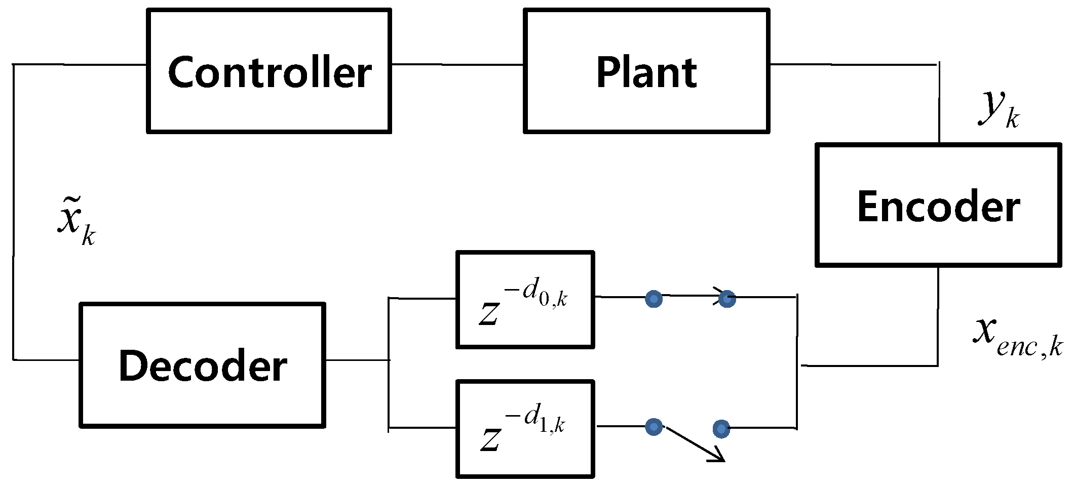
We consider a control system where sensor measurements are encoded and transmitted over two channels alternatively. Only one channel will be active at a time while the other channel is ready. To provide robust operation, the system may support heterogeneous communication protocols. For example, information may be transmitted over Wi-Fi while the 5G network is ready, and vice versa. A corresponding closed-loop system model is shown in Figure 1. The state equation for the given system can be given as
where the is a state vector, is a measurement vector, is a control signal. It is assumed that process noise and measurement noise are normally distributed with zero mean and covariance matrices, and , respectively. In Figure 1, encoding and decoding are considered from the perspective of communication. The measurement signal is transformed to generate the encoded signal . The encoded signal will be transmitted through the channel which has delay . If channel experiences an excessive delay, it switches the transmission to channel which has delay The delay can be decomposed into the transmission delay and delay due to consecutive packet errors, . It is assumed that these two different types of delay are independent. The decoder generates the decoded signal , serving as the final estimate of the state .

Figure 1.
A system model where represents a channel with a delay .
To determine the control signal, we consider an LQG control. A cost function of the LQG control with a finite time horizon can be given as
where is a transpose of the vector , is the weight matrix for the terminal state, and and are nonnegative definite weight matrices for running states and controls, respectively. To derive optimal control, a conventional value function associated with dynamic programming can be defined as follows.
Equation (4) can be easily further derived as the following recursion
Equation (5) can be rearranged as
where . Since is a quadratic function of , the optimal control signal can be easily calculated as
After inserting (7) into (6), can be represented as a quadratic form of from which the Riccati equation can be given as
While the optimal control in (7) is expressed as a linear transform of , perfect state information may not be available due to packet error or delay. Thus, the estimation of the state will be required in consideration of the communication structure in the control system.
3. Design of Encoder and Decoder for a Delayed Channel with a Packet Error
To design an optimal controller, we adopt the encoder and decoder model, which is frequently used in the development of LQR and LQG controllers [18,25]. The Kalman filter is utilized as the encoding method, which has been demonstrated to be optimal for LQG control across a packet-dropping link [18]. The state estimation at time with Kalman filter can be given as
where is the prediction of the state at time with information available up to . Since the encoder simply takes the Kalman filter, the encoder equation can be given as
The decoder can be designed with a predictive form as follows.
where is a packet delay at time , and is a variable for packet arrival at time which has 1 for successful packet arrival, otherwise 0.
To assess the proposed encoding and decoding scheme, we need to analyze the characteristics of several errors. We start with the decoding error , which is defined as
When the packet is received successfully, the decoded state is in predictive form using . Thus, needs to be in the same form to find a more manageable form. It can be easily derived as
With (13), can be arranged as
where .
It is noted that (14) can be considered as a generalization of the result in [18] where the term in (14) is 0 when the delay is 0. Whether the packet is received successfully or not, depends on since encoding is simply Kalman filtering. This model is applied to the system described in Figure 1 since the channel is transparent to the encoder and decoder while has dependency on the active channel.
4. Channel Switching Algorithms
To maintain a control system operating on a network reliably, it is important to effectively manage the channels. While various channel management schemes exist, we focus on channel switching which allows the system to receive information from a single channel at a time for simplicity. Thus, the channel environment we consider throughout this paper is fundamentally different from one in many existing literature in the sense that they have developed efficient exploitation of the delayed information from multiple channels with the assumption that multiple channels are always active.
After decoding at the decoder, the control signal can be determined from LQR control as
where . By inserting (15) into (1), (1) can be arranged as
where , which we call effective noise since it includes the process noise and errors due to estimation error.
The effective noise can be considered as an equivalent process noise. Thus, the power of the effective noise has a direct effect on the quality of control. In this perspective, we can define stability for practical consideration as follows.
Definition 1
( stability). Let denote the covariance matrix of the effective noise in the state equation in (16) at time . stability is achieved, if where is the trace of the matrix in the bracket.
In other words, the control system achieves α stability when the variance of the effective noise is lower than the specified threshold α. To find a switching criterion to satisfy the stability, we first define state estimation error
Since the time instance of the encoded signal is with the successful reception of the packet at time the predictive form of the state vector at time using can be easily derived as
With (17) and (18), can be calculated as
where which is the estimation error of the Kalman filter. Some interesting observations can be made from the comparison between (14) and (19). The process noise influences while it does not influence since the decoding error depends on the channel and the method of decoding. When the information packet is successfully received, both equations are not in a recursive form due to the resetting effect of the newly arrived packet.
Let the covariance matrix of be denoted by . When , has the following relation from (19).
where is the covariance of the state estimation error using the Kalman filter at time . Finally, since from (16), can be expressed as
From (20) and (21), several interesting observations can be made. When is unstable, the error covariance increases with the . has a bounded value as long as has the finite maximum value due to the effect of resetting with the successful arrival of the packet. Even though may be stable, outdated information with delay increases the error covariance.
With (21), the delay condition to guarantee the stability can be given as follows.
Theorem 1.
Let be . If where is the most recent time when decoding was successful at time , then the stability is guaranteed for the system described in Figure 1 with the condition that at least one information packet is received successfully at time .
Proof of Theorem 1.
From the definition, . With the condition that at least a single information packet is received successfully at time , the covariance of the estimation error can be easily calculated from (20) as
Since which is taken from (21) and (22), and if , then stability is achieved by definition, which proves the proposition. □
It is noted that this proposition is generic since it does not assume a particular channel-switching algorithm. Similarly, the asymptotic condition for stability can be posed as follows.
Theorem 2.
With the asymptotic condition, If where , and , then the stability is guaranteed for the system described in Figure 1.
Proof of Theorem 2.
Since is the estimation covariance at time without delay, this corresponds to . Since asymptotically converges to , can be given by . Due to the non-negative definiteness of the covariance matrix, monotonically increases with . Thus, has the maximum value at a time when it has a maximum delay at the asymptotic region, which proves the theorem. □
Theorem 2 implies that the maximum delay determines the stability in the asymptotic region. From the Theorem 2, the maximum delay to guarantee the stability in the asymptotic region can be given as follows.
Proposition 1.
Proof of Proposition 1.
It can be trivially proved by following the procedures for the proofs in Theorems 1 and 2. □
From Proposition 1, it is expected that the channel switching can guarantee the stability as long as appropriate channel switching is applied for some specific channel conditions by limiting the maximum delay to . Exploiting this observation, a conventional global threshold switching (GTS) algorithm can be given as follows.
whereis the active channel indicator at time and is a nonnegative integer parameter, which has an effect on the performance and the switching characteristics. It is noted that switching is determined with the same threshold. Thus, this algorithm can be applicable without exploiting statistical knowledge of the channels.
While the GTS algorithm can be configured without the knowledge of the channel statistics, it may stay at a worse channel for a long time. To overcome this drawback, depending on the knowledge of channel statistics, two algorithms are proposed. The first algorithm aims to exploit information on the maximum transmission delay. With the assumption that the maximum transmission delays at both channels are available, it can be advantageous to use the channel with a smaller maximum transmission delay. In this context, the local threshold switching (LTS) algorithm can be described as
where , is a non-negative integer parameter, and is an indicator function, the value of which is 1 when the condition inside the bracket is true, otherwise it is 0. It is expected that setting the as smaller for a channel with a larger maximum transmission delay can result in using the channel with a smaller maximum transmission delay more often.
The LTS algorithm is built on the underlying assumption that the two channels have a similar degree of packet error rate (PER). Thus, it may not provide good performance when the channel with a larger transmission delay has a low PER, and the other channel with a smaller transmission delay has a high PER. To address this limitation and leverage both the maximum transmission delay and PER for channel switching, an alternative algorithm, known as the advanced local threshold switching (ALTS) algorithm, is introduced as follows.
where is a nonnegative integer, and is PER at channel This algorithm simply considers one additional channel statistics, which is the PER. It reduces the threshold for switching to the channel with a lower PER so that the preference for the channel with a low PER can be formed when the maximum transmission delays are comparable.
Regardless of the types of the proposed algorithm, the channel condition to guarantee the stability can be given as follows.
Proposition 2.
On the condition of
,
where
is the maximum consecutive packet error on channel
, all the proposed threshold switching algorithms guarantee the
stability.
Proof of Proposition 2.
From the condition , needs to be satisfied for which proves the proposition. □
While Proposition 2 provides the channel condition to guarantee the stability for all switching algorithms, depending on the value of and the channel characteristics, stability may never be achieved. To tackle this issue, we define a probabilistic stability as a tool for characterizing the proposed switching algorithms further.
Definition 2
( probabilistic stability). We define as probabilistic stability that stability is achieved with the probability of where .
With probabilistic stability, the proposed switching algorithms can be compared consistently in the following way.
Theorem 3.
Let the probabilistic stability of the GTS algorithm and the LTS algorithm be denoted by and respectively. It is assumed that for . When where and is the probability that the active channel is j with the algorithm denoted by , .
Proof of Theorem 3.
By definition, = + where denotes the probability that the channel is an active channel with the global threshold switching algorithm. can be equivalently expressed as where | . Thus, we can express as
We consider . Due to the symmetricity, the same argument can be applied to the opposite case. We can express and as follows.
From (27) and (28), can be easily derived as
Similarly, and can be derived as
can be arranged as
where . Since and which is evident from (29) and (30). Since due to , follows. □
From Theorem 3, we can identify channel conditions favoring one algorithm over the other in terms of probabilistic stability.
Proposition 3.
When and
and there is no packet error in both channels, the LTS algorithm provides better probability stability than the GTS algorithm.
Proof of Proposition 3.
This proposition directly follows from Theorem 3. □
Proposition 4.
When packet error occurs with a constant packet error rate and there is no transmission delay at both channels, the ALTS algorithm provides better probability stability than the LTS algorithm does.
Proof of Proposition 4.
Since it is assumed that there is no transmission delay, follows the geometric distribution with parameter . We consider the case the opposite case will be proven with the same argument. When , . Thus, to satisfy , the condition of needs to be satisfied. Since follows the geometric distribution, and can be expressed as follows.
It is evident that as long as is a positive integer and and are set to the same value for both thresholds, . Since and . □
Proposition 5.
When packet error occurs with a constant packet error rate and both channels have the same fixed transmission delay or uniform random delay with the same maximum delay, the LTS algorithm provides better probabilistic stability than the GTS algorithm.
Proof of Proposition 5.
When both channels have the same fixed transmission delay, following the similar arguments made in the Proof of proposition 4, it can be trivially proved. can be expressed as
where and are transmission delay and delay due to consecutive packet error in channel at time. When both channels have uniform random transmission delay with the same maximum transmission delay, the probability of the delay at channel can be given as
By exploiting the independence between and from the assumption, it can be expressed as
From the assumption of the uniform distribution of the transmission delay, it can be further arranged as
where Since this probability does not depend on the threshold, but on the PER, we again consider as in the Proof of the proposition 4. When , from the fact that Pr depends on the distribution of the delay from the consecutive packet errors. Thus, to satisfy , the condition of needs to be satisfied. From the Proof the Theorem 1, . Thus, . □
Proposition 6.
When packet error occurs with a constant packet error rate and there is a fixed same transmission delay or uniform random delay with the same maximum delay at both channels, the ALTS algorithm provides better probabilistic stability than the LTS algorithm.
Proof of Proposition 6.
Following the same procedure as in the Proof for the proposition 5, it can be shown that when , . Thus, to satisfy , the condition of needs to be satisfied.
It is evident from the above equation that as long as and and are set the same value for both thresholds, . Thus, . □
Although the ALTS algorithm demonstrated superior performance in specific channel conditions, it is crucial to identify generic conditions under which one algorithm outperforms the other.
Lemma 1.
With .
Proof of Lemma 1.
Based on the Proof of Theorem 3, and to satisfy ,
Equation (40) can be arranged as
which proves the lemma. □
Several important observations can be drawn from this lemma. To satisfy the inequality, both terms need to have value with the same sign, that is, when , . This implies that the switching algorithm must set a threshold to favor the channel where a smaller delay occurs with a higher probability. The LTS algorithm accomplishes this by reducing the threshold for the channel with a probabilistically larger delay. However, since the penalty decision is made based on the maximum transmission delay only, the LTS algorithm may fail to provide better performance than the GTS algorithm for some channel conditions due to the limited knowledge of the channel. The GTS algorithm can be considered as a special case of the LTS algorithm. Thus, if is determined with information on the statistical characteristic of the channels such that , the LTS algorithm can perform better than the GTS algorithm.
Similarly, we provide a condition in which the ALTS algorithm performs better than the LTS algorithm.
Lemma 2.
With .
Proof of Lemma 2.
It can be proved by following the same procedure for the Proof of the Lemma 1. □
The condition for Lemma 2 requires that the switching algorithm needs to set a threshold such that it can stay longer at a channel where a smaller delay occurs with a higher probability. The ALTS algorithm is required to set three parameters properly with the information on the maximum transmission delay and the packet error rate. The LTS algorithm can be considered as a special case of the ALTS switching algorithm. Thus, if and are determined such that , the ALTS algorithm will perform better than the LTS algorithm by choosing properly while setting the and the same as those of the LTS algorithm.
5. Simulation Results
In this section, we assess the performance of the proposed channel-switching algorithms through numerical simulation. To this end, the system model for an inverted pendulum was adopted [26,27]. Corresponding matrices are as follows.
This system is an unstable one. The maximum eigenvalue of the system matrix is 1.8257. and are set as and respectively. The finite horizon was set as 1000 and 100 different realizations were generated. The probabilistic stability was calculated by counting the occurrence of the case that the sum cost is less than the target sum cost and dividing it by 100,000. It is also assumed that transmission delay is uniformly distributed with the maximum delay being specified for each channel, and a packet error with a given packet error rate occurs independently at each time instance.
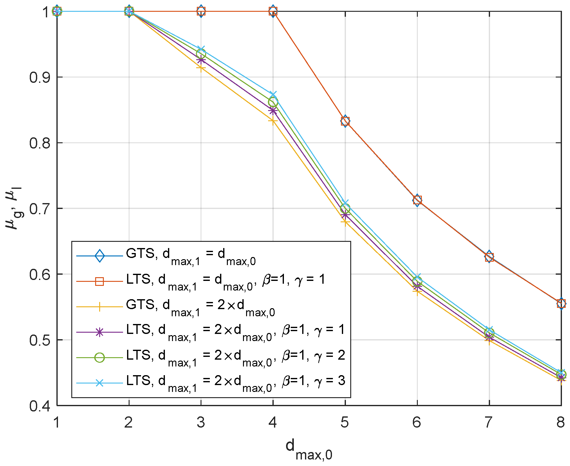
Several experiments have been executed to verify the validity of the analysis and the basic characteristics of the proposed algorithms. The comparison of the probabilistic stability between GTL and LTS is shown in Figure 2, where is set to 4. and were set to 0 to assess the effect of the delay on performance without being interfered by additional system conditions. When both channels have the same transmission delay, GTS and LTS exhibit similar performance, irrespective of the maximum transmission delay. When max( is less than equal to , both and are 1. However, as max( increases beyond , and decrease inversely proportional to max(. It is also observed that they have the same value as expected since the channels, 0 and 1 have the same maximum delay. However, when , some interesting observations can be made. LTS reduces the instability cases by 14.3%, 9.24%, 3.38%, 1.81%, 1.04%, and 0.80% for ranging from 3 to 8, respectively. The benefit of LTS is found to decrease as increases. This is unavoidable since the instability region increases as increases, which decreases the ratio of instability region between GTS and LTS. This figure also shows the effect of . As increases, it provides better performance as the large enforces the control system to operate on channel 0 more often.
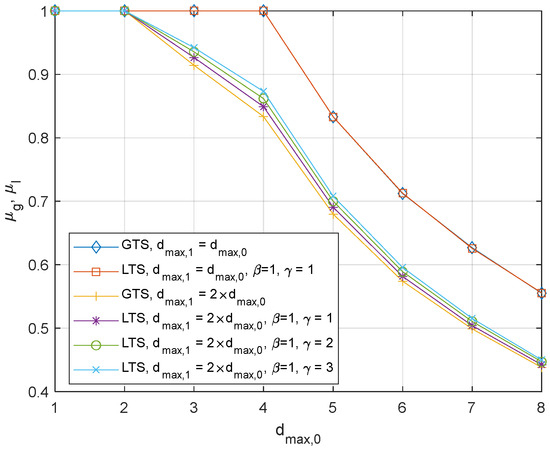
Figure 2.
The probabilistic stability of the GTS, and LTS, where and .
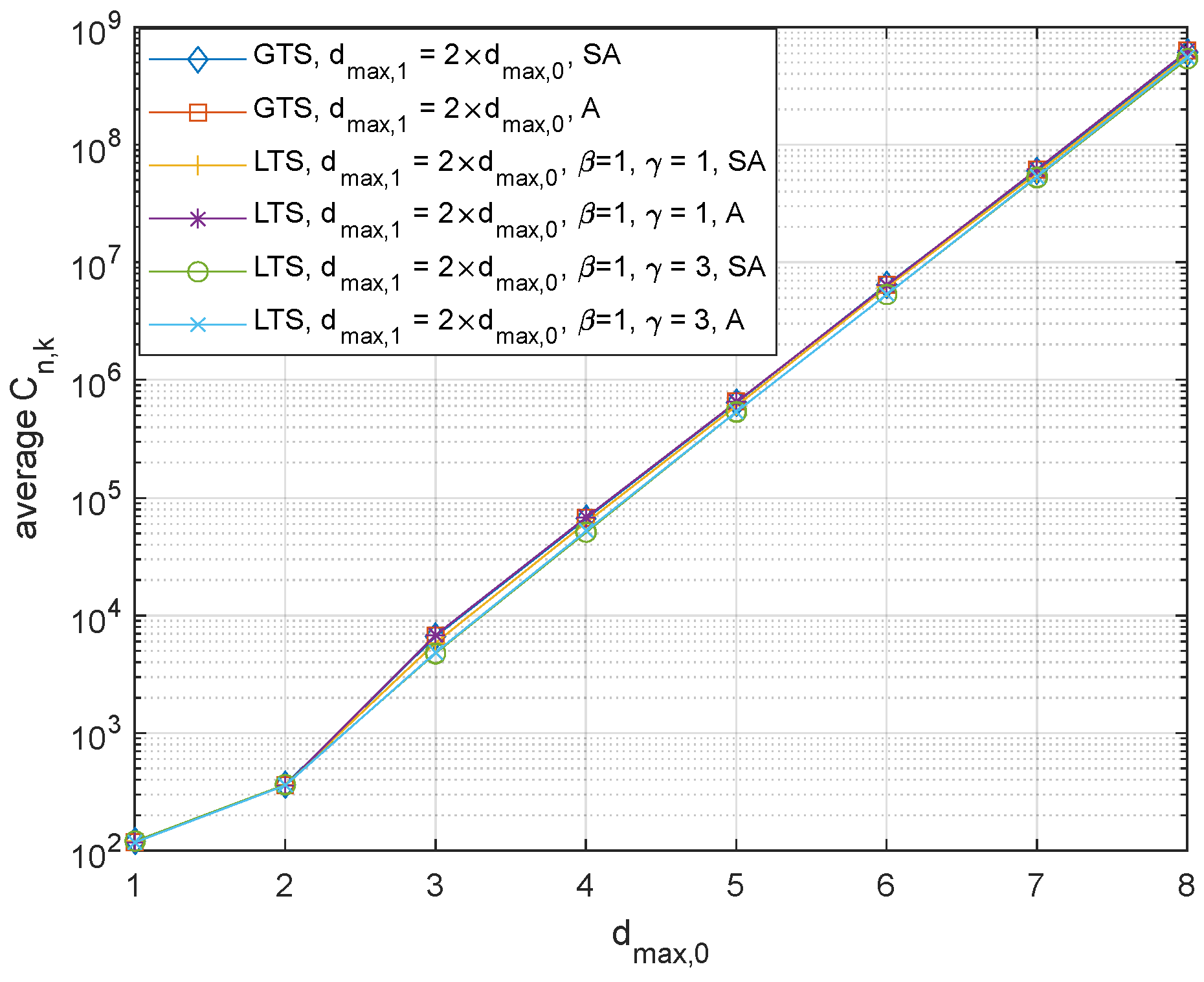
Figure 3 shows the average for the same setting as in Figure 2. This result verifies that the analysis results based on (21) tightly match with the sample averages. While the distinction may not be easily noticeable in the figure, LTS provides a lower variance of the effective noise than GTS for the asymmetric channel while they have almost identical values for the symmetric channel. It is also observed that the performance gain by setting larger is significant. More specifically, while the performance gains of the LTS over GTS are 12.7%, 8.63%, 6.49%, 4.81%, 4.77%, and 4.29% for ranging from 3 to 8, respectively, when = 1, they are 28.6%, 23.1%, 17.8%, 16.1%, 12.5%, and 11.8% when = 3. This result is in line with the result for probabilistic stability.
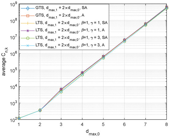
Figure 3.
The probabilistic stability of the GTS, and LTS, where and (SA: Sample average; A: Analysis).
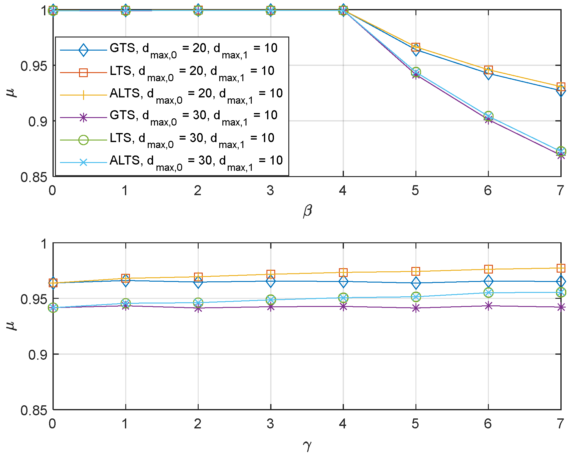
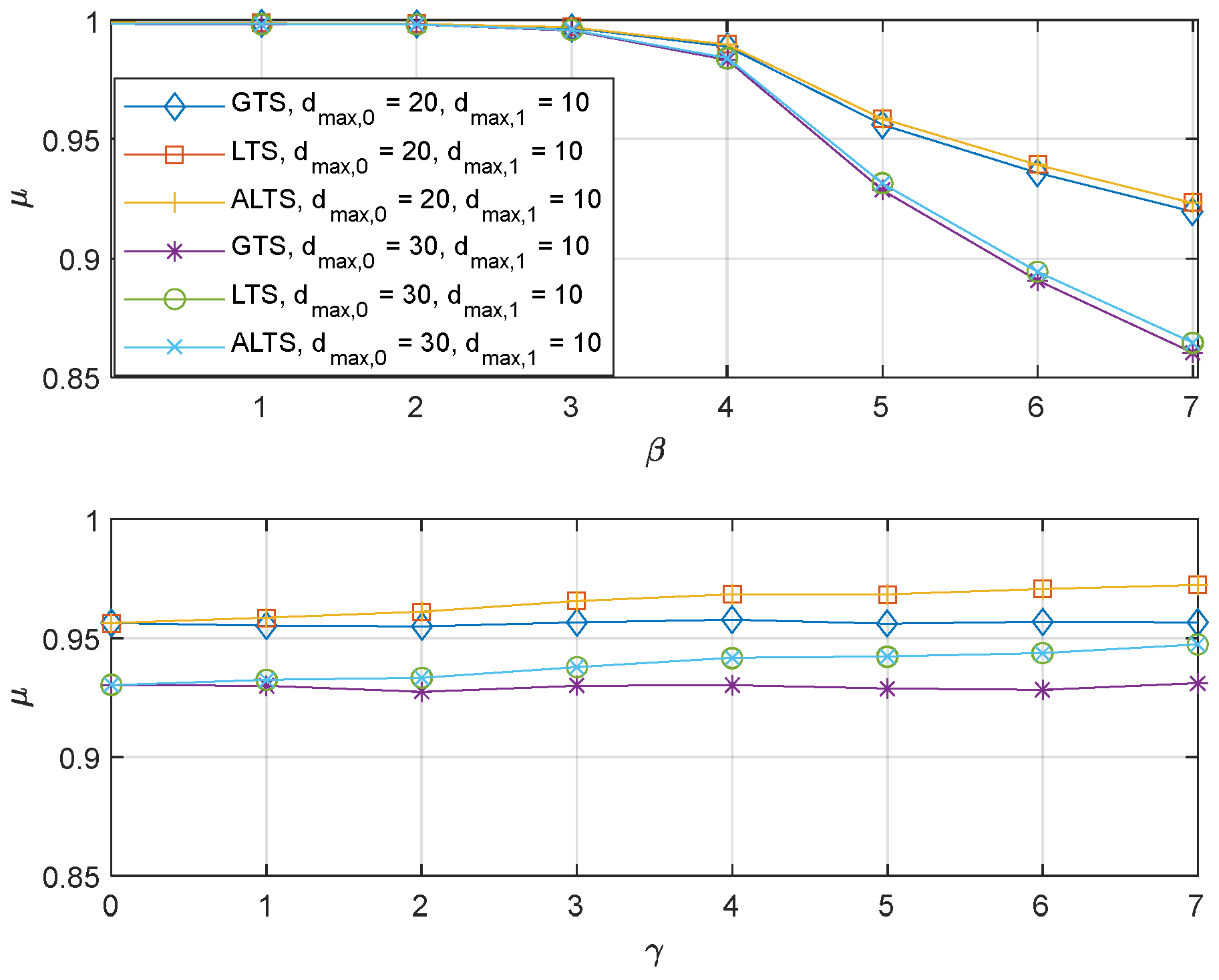
The effect of parameters for the proposed algorithms on the performance with is shown in Figure 4. Default values for and were set to 1 unless the algorithm was evaluated for different parameter values. The plot on top shows the effect of . It is observed that the performance degrades more as increases. A large increases the probability of switching to a worse channel. That is, when the is greater than or equal to 4, the probability of switching to a worse channel becomes non-zero since the threshold for switching becomes 10 or lower. It is also observed that for the same parameter, the performance of the proposed algorithm depends on the maximum transmission delay. This dependence is primarily attributed to the intrinsic nature of the problem rather than the proposed algorithm itself since the larger maximum delay increases the occurrence of a delay larger than . As expected, LTS and ALTS have the same performance since PER is the same, which sets as 0. The plot at the bottom shows that as increases, the performance of the LTS and ALTS improves. A large lowers the threshold for switching from a bad channel to a good channel, which creates an implicit preference for a good channel. Figure 5 show the experiment results with different PER, . The same trend with each parameter can be observed. The only noticeable difference is that the probabilistic stability is found to degrade a little bit due to the packet error. It is also interesting to note that when is high, the performance depends more on the maximum delay rather than the PER.
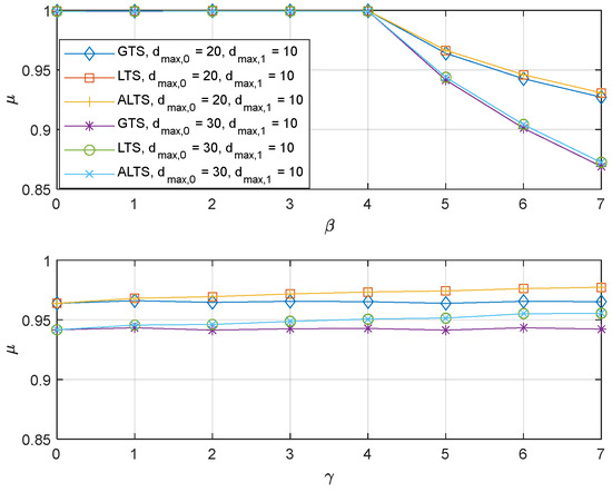
Figure 4.
The probabilistic stability of the GTS, LTS, and ALTS where and .
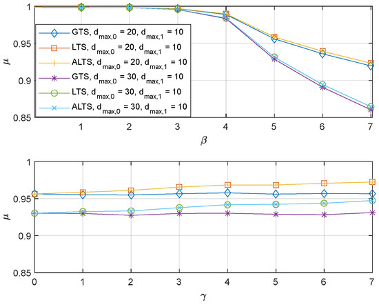
Figure 5.
The probabilistic stability of the GTS, LTS, and ALTS where e and .
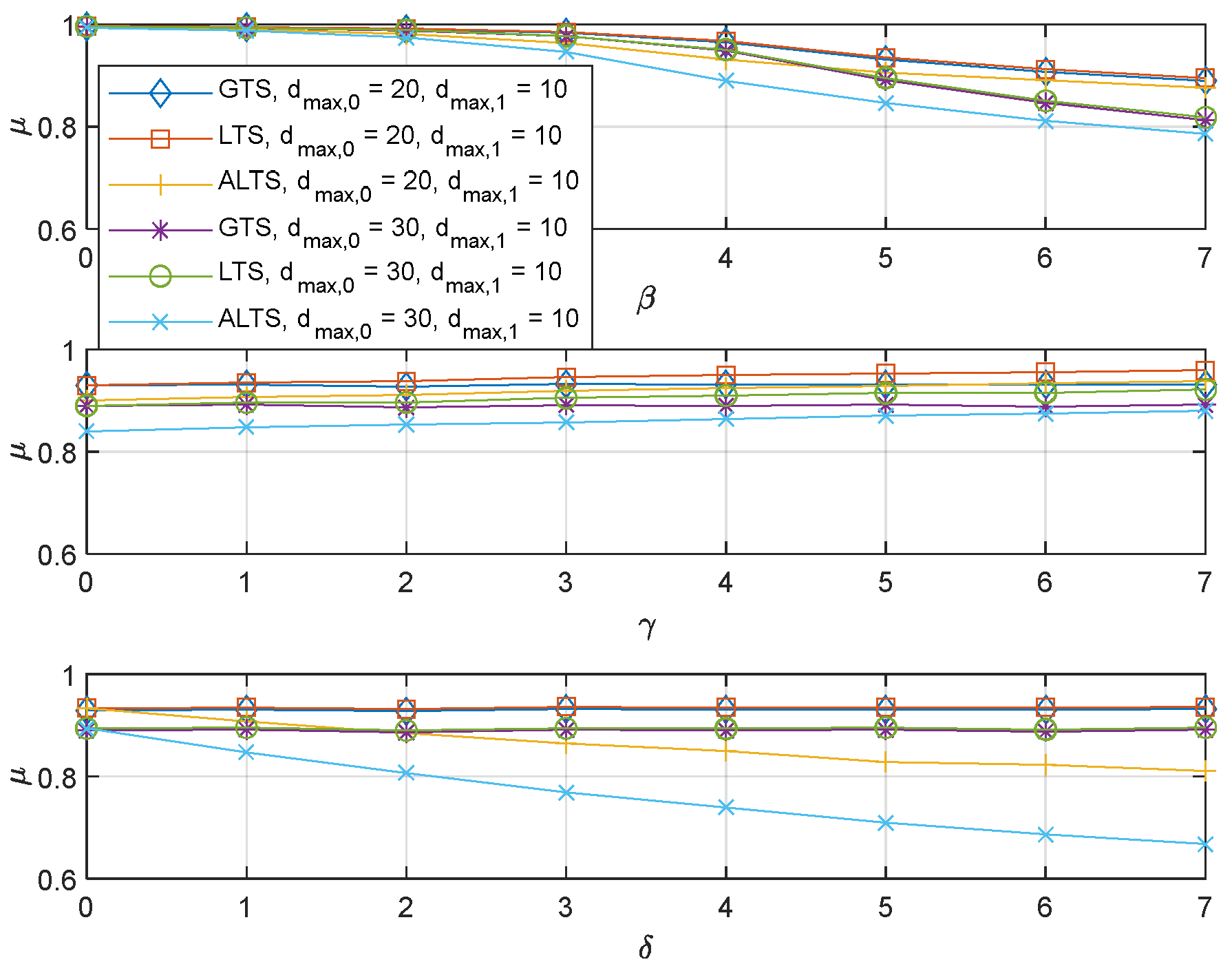
The ALTS algorithm was proposed to improve the performance when there is asymmetricity in the packet error rates over two channels. However, asymmetry in the packet error rate can be further classified into synchronous cases so that a channel with a larger maximum transmission delay has a larger PER, and asynchronous cases so that a channel with a larger maximum transmission delay has a smaller PER. The performance of the proposed algorithms was assessed for the synchronous case in Figure 6, where and . It is observed that the performance trends for GTS and LST are pretty much similar to those observed in the preceding experiments. However, ALTS is found to perform poorly in comparison with GTS and LTS. In addition, the performance of ALTS degrades further with increasing. It is because creates an implicit preference for a channel with a larger maximum delay in the given system configuration while the delay has a more significant effect on performance than PER. This result brings attention to a need for the remedy on ALTS such that it can perform robustly to many different system configurations. When ALTS is applied to the synchronous case, the expected performance improvement with increasingcan be observed in Figure 7.
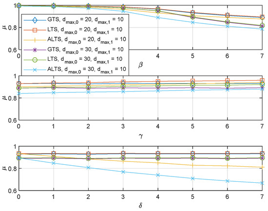
Figure 6.
The probabilistic stability of the GTS, LTS, and ALTS, where and .
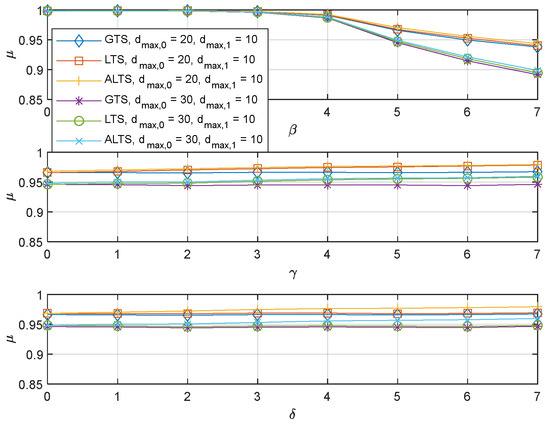
Figure 7.
The probabilistic stability of the GTS, LTS, and ALTS, where and .
One heuristic modification has been made to make ALTS operate robustly for many different system environments. A pseudo-global maximum delay, can be defined such that it can represent the maximum effective channel delay in consideration of PER.
where . is the average delay due to the packet error which is easily calculated from geometric distribution. The dividing factor 2 is introduced heuristically to limit the effect of the in determining . Exploiting the new measure, the threshold for the ALTS can be modified into
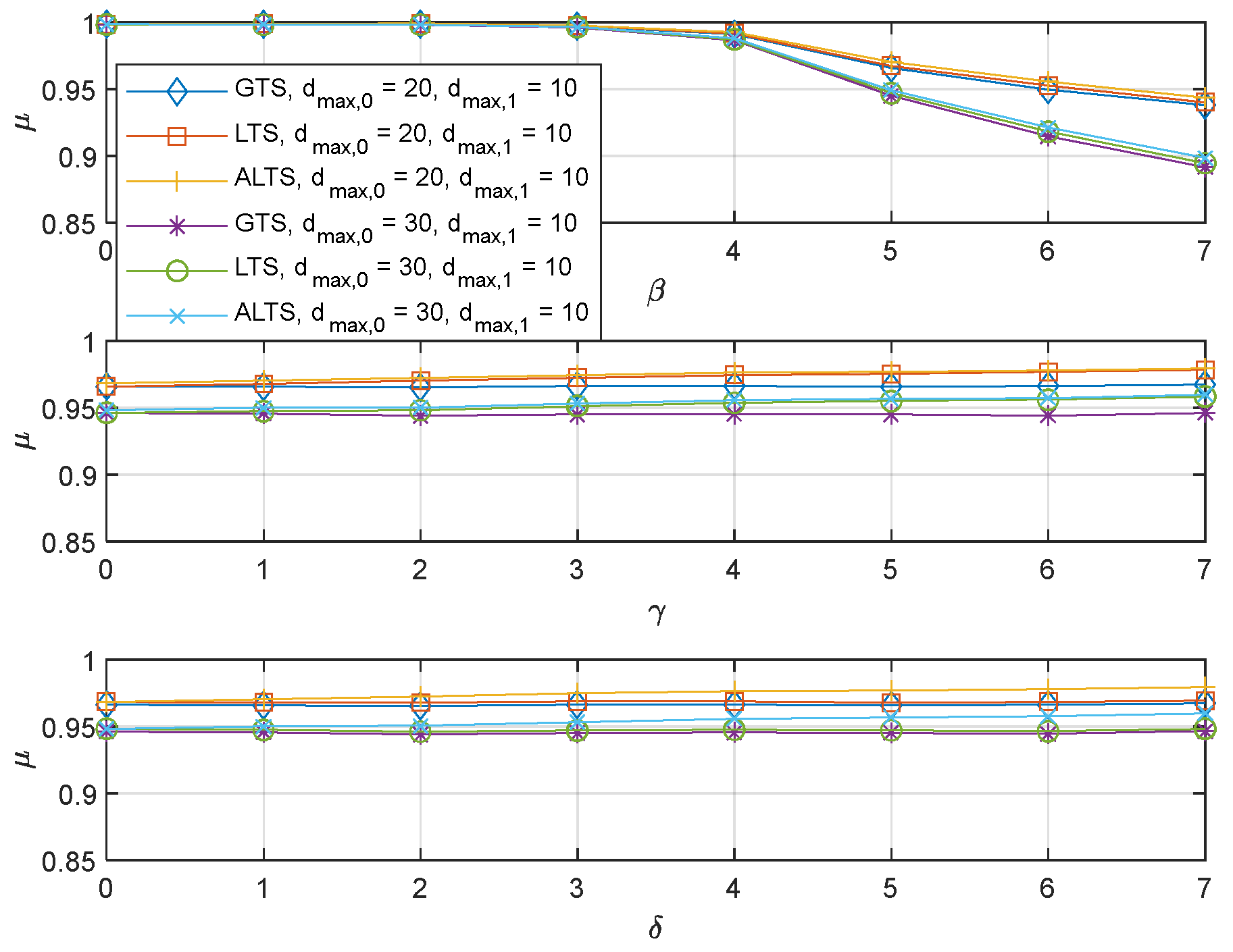
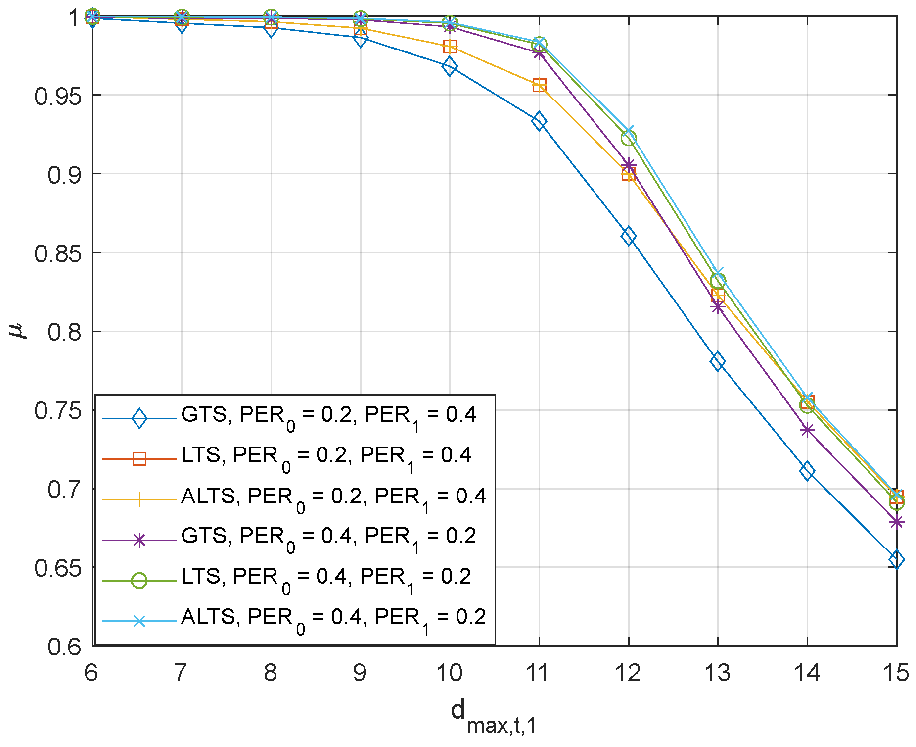
in (43) was added to ensure that can be applied when the current channel environment corresponds to the synchronous case. To assess the robust performance of ALTS over different system environments, numerical experiments were executed over various maximum transmission delays and various packet error rates in Figure 8 and Figure 9. Since in Figure 8, the asymmetric case occurs when is smaller than . In this case, will be effectively set as 0 due to the . Thus, LTS and ALTS will provide the same performance as observed in Figure 8. However, when is smaller than , the application of in ALTS is found to improve LTS. Similarly, the asymmetric case occurs when and , since . Even though the performances of LTS and ALTS are hardly discernible in the symmetric case due to the resolution of the plot, ALTS provides the reduction of 9.2%, 14.8%, 13.7%, 12.8%, 9.81%, 7.58%, 4.49%, and 2.49% in terms of the number of occurrences of an unstable state. The experiment results in Figure 8 and Figure 9 verify that with a simple modification, ALTS improves performance over LTS for the symmetric case while its performance is the same as that of the LTS in the asymmetric case.
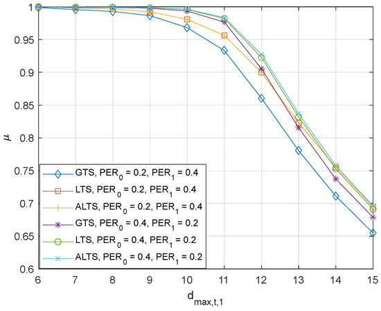
Figure 8.
The probabilistic stability of the GTS, LTS, and ALTS, where , and .
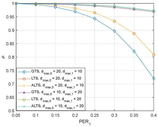
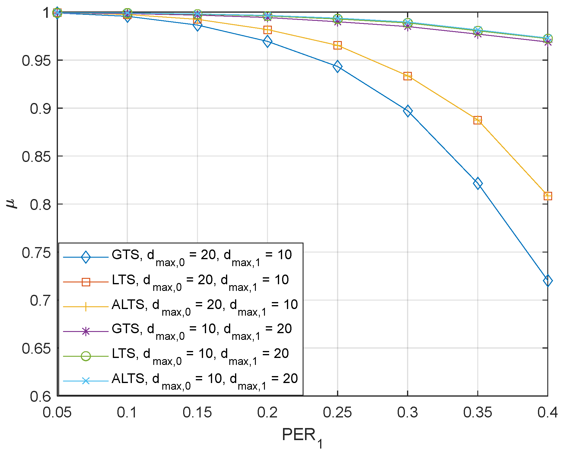
Figure 9.
The probabilistic stability of the GTS, LTS, and ALTS, where = and .
Finally, we evaluated the proposed algorithms under more realistic operating conditions, incorporating channel parameters derived from the existing literature. Two channels were assumed to be 5G cellular link and Starlink. The end-to-end latency of 5G-enabled internet was measured to be 24 msec on average, with a maximum of 29 msec [28]. Based on this information, the 5G channel was approximated to have a uniform distribution from 20 msec to 30 msec with a PER of 10−5, a commonly used target PER in 5G systems. The measured PER for Starlink ranges from 0.45% to 1.96%, while its latency is around 50 msec in the median, with the first quantile at 40 msec and the third quantile at 60 msec [29]. Utilizing this information, the Starlink channel was approximated to have a uniform distribution between 30 msec and 70 msec, with a PER of 0.01. For comparison with an optimal approach that exploits information from both channels, the method for optimal sensor scheduling in [30] was adapted, allowing the selection of the channel with the lower variance of the effective noise at each time step. We refer to this algorithm as the Oracle algorithm. It is important to note that the Oracle algorithm exploits instantaneous delay information from both channels, while the proposed algorithms use the instantaneous delay information from the currently active channel only.
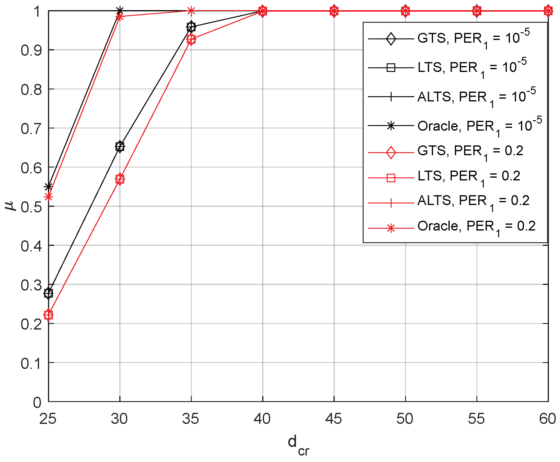
Figure 10 depicts the performance of the proposed algorithms for this more realistic operational case under two different scenarios. The parameters for the proposed algorithm were heuristically chosen as and . The finite horizon was set at 1000, and 1000 different realizations were generated to evaluate performance. The first scenario assumes normal operating conditions for both channels, while the second scenario characterizes the poor channel condition of the 5G channel with a PER of 0.2. The proposed algorithms are shown to provide comparable performance to the Oracle algorithm for a wide range of values for both scenarios. When is small, there can be frequent switching between the 5G channel and Starlink channel for proposed algorithms, while the Oracle algorithm selects the best channel instantaneously, resulting in a noticeable difference. However, when is greater than 30, as long as the proposed algorithm switches to the 5G channel with smaller delays, it is likely to stay there unless long consecutive packet errors occur. Thus, the probabilistic stability of the proposed algorithm becomes almost the same as that of the Oracle method for large . Since discerning performance with a larger in Figure 10 is challenging, Table 1 is introduced, presenting the count of cases where the delay is larger than . While the Oracle algorithm avoids encountering an unstable state for larger , the proposed algorithms may experience occasional instances of instability. It occurs before it stays at the 5G channel with a shorter delay. It is also observed that LTS and ALTS have fewer occurrences due to the additional parameters, which accelerate switching to a better channel than GTS. These results demonstrate that the proposed algorithms provide better performance than the conventional method while achieving near-optimal performance in some cases.
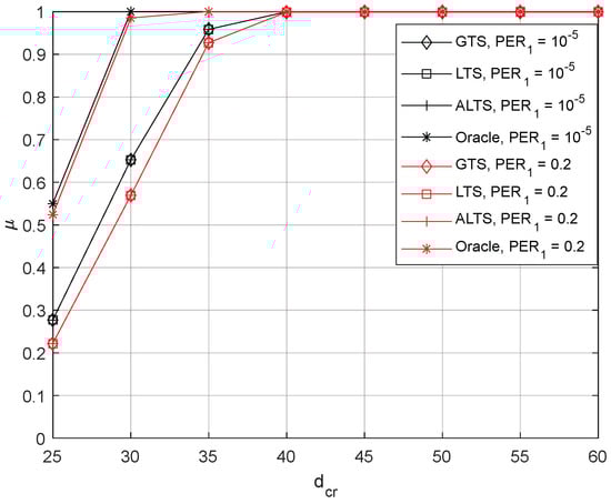
Figure 10.
The probabilistic stability of the GTS, LTS, ALTS, and Oracle, where and = 0.01.

Table 1.
The number of times that the delay is greater than dcr in Figure 10.
6. Conclusions
In this paper, we introduced two channel switching algorithms to enhance the robustness of networked control systems facing delays and packet errors. Leveraging the framework of the LQG controller and an encoder–decoder structure for channel modeling, we derived a crucial decoder error covariance matrix, pivotal for informed channel switches to maintain α stability. Addressing practical challenges, we further introduced probabilistic stability. Specific conditions wherein the proposed algorithm excels in terms of probabilistic stability have been identified. Simulation results not only confirmed the superior performance of the proposed switching algorithms but also demonstrated their potential to achieve near-optimal performance despite utilizing limited information.
While our proposed algorithm is well-suited for multiple channels with a delay, it assumes accurate delay information. However, uncertainties in delayed information can arise due to processing time or delay from the physical structure. Moreover, while synchronous channels were implicitly assumed throughout this paper, the proposed algorithm may not be trivially applied to asynchronous channels. Due to the lack of strict timing in asynchronous channels, there can be variations in the timing of data arrivals. This unpredictability poses a challenge for algorithms that rely on precise timing information. Even though those delays can be estimated, the estimate may not be accurate. To address the delay uncertainty, a robust channel-switching algorithm needs to be further investigated. One may consider exploiting deep reinforcement learning, which can perform robustly with uncertainty and actively respond to the variation in channel environments. The scheduling issue also needs to be studied when multiple devices need to be controlled over a network where a scheduling policy has an impact on the delay of each channel.
Funding
This research received no external funding.
Data Availability Statement
Data are contained within the article.
Conflicts of Interest
The author declares no conflicts of interest.
References
- Mezaal, Y.S.; Yousif, L.N.; Abdulkareem, Z.J.; Hussein, H.A.; Khaleel, S.K. Review about effects of IOT and Nano-technology techniques in the development of IONT in wireless systems. Int. J. Eng. Technol. 2018, 7, 3602–3606. [Google Scholar]
- Sheng, Z.; Tian, D.; Leung, V.C.M.; Bansal, G. Delay Analysis and Time-Critical Protocol Design for In-Vehicle Power Line Communication Systems. IEEE Trans. Veh. Technol. 2018, 67, 3–16. [Google Scholar] [CrossRef]
- Fridman, E. Tutorial on Lyapunov-based methods for time-delay systems. Eur. J. Control 2014, 20, 271–283. [Google Scholar] [CrossRef]
- Gu, K.; Niculescu, S.I. Survey on Recent Results in the Stability and Control of Time-Delay Systems. J. Dyn. Syst. Meas. Control 2003, 125, 158–165. [Google Scholar] [CrossRef]
- Lu, X.; Zhang, Q.; Liang, X.; Wang, H.; Sheng, C.; Zhang, Z. Optimal control for networked control systems with multiple delays and packet dropouts. Int. J. Adv. Robot. Syst. 2020, 17, 1–8. [Google Scholar] [CrossRef]
- Xu, J.; Zhang, H.; Gu, G.; Tang, Y. Stabilization of Discrete-Time Systems with Random Delays and Packet Drops: A Predictor-Like Controller. SIAM J. Control Optim. 2023, 61, 1737–1759. [Google Scholar] [CrossRef]
- Zhang, W.; Branicky, M.S.; Phillips, S.M. Stability of Networked Control Systems. IEEE Control Syst. Mag. 2001, 21, 84–99. [Google Scholar] [CrossRef]
- Delavar, R.; Tavassoli, B.; Beheshti, M.T.H. Improved Stability Analysis of Nonlinear Networked Control Systems over Multiple Communication Links. In Proceedings of the Iranian Conference on Electrical Engineering, Tehran, Iran, 2–4 May 2017. [Google Scholar]
- Zhu, X.; Yang, G.H. State feedback controller design of networked control systems with multiple-packet transmission. Int. J. Control 2009, 82, 86–94. [Google Scholar] [CrossRef]
- Wen, D.L.; Gao, Y. H∞ Controller Design for Networked Control Systems in Multiple-Packet Transmission with Random Delays. Appl. Mech. Mater. 2013, 278–280, 1601–1604. [Google Scholar] [CrossRef]
- Mager, F.; Baumann, D.; Jacob, R.; Thiele, L.; Trimpe, S.; Zimmerling, M. Feedback Control Goes Wireless: Guaranteed Stability over Low-power Multi-hop Networks. In Proceedings of the 10th ACM/IEEE International Conference on Cyber-Physical Systems, Montreal, QC, Canada, 16–18 April 2019; pp. 97–108. [Google Scholar]
- Xu, J.; Gu, G.; Tang, Y.; Qian, F. Channel modeling and LQG control in the presence of random delays and packet drops. Automatica 2022, 135, 109967. [Google Scholar] [CrossRef]
- Garone, E.; Sinopoli, B.; Goldsmith, A.; Casavola, A. LQG Control for MIMO Systems over Multiple Erasure Channels with Perfect Acknowledgment. IEEE Trans. Autom. Control 2012, 57, 450–456. [Google Scholar] [CrossRef]
- Lu, X.; Cai, Y.; Wang, H.; Wang, H.; Zhang, G.; Liang, X. Necessary and Sufficient Condition of Optimal Control for Networked Control Systems with Markovian Packet Dropout. Int. J. Control Autom. Syst. 2023, 21, 1485–1492. [Google Scholar] [CrossRef]
- Chen, F.; Zhou, X. Design of predictive controller for Networked Control Systems. In Proceedings of the 2023 IEEE 6th Information Technology, Networking, Electronic and Automation Control Conference (ITNEC), Chongqing, China, 24–26 February 2023. [Google Scholar]
- Tian, Z.; Wang, Y. Predictive control compensation for networked control system with time-delay. Proc. Inst. Mech. Part I J. Syst. Control Eng. 2022, 236, 107–124. [Google Scholar] [CrossRef]
- Sinopoli, B.; Schenato, L.; Franceschetti, M.; Poolla, K.; Jordan, M.; Sastry, S. Optimal control with unreliable communication: The tcp case. In Proceedings of the American Control Conference, Portland, OR, USA, 4–6 June 2005. [Google Scholar]
- Gupta, V.; Spanos, D.; Hassibi, B.; Murray, R.M. On LQG control across a stochastic packet-dropping link. In Proceedings of the American Control Conference, Portland, OR, USA, 4–6 June 2005. [Google Scholar]
- Gupta, V.; Dana, A.F.; Hespanha, J.P.; Murray, R.M.; Hassibi, B. Data Transmission Over Networks for Estimation and Control. IEEE Trans. Autom. Control 2009, 54, 1807–1819. [Google Scholar] [CrossRef]
- Liang, X.; Xu, J.; Zhang, H. Optimal Control and Stabilization for Networked Control Systems with Packet Dropout and Input Delay. IEEE Trans. Circuits Syst. II Express Briefs 2017, 64, 1087–1091. [Google Scholar] [CrossRef]
- Sinopoli, B.; Schenato, L.; Franceschetti, M.; Poolla, K.; Sastry, S. LQG control with missing observation and control packets. In Proceedings of the 16th IFAC World Congress, Prague, Czech Republic, 3–8 July 2005. [Google Scholar]
- Sinopoli, B.; Schenato, L.; Franceschetti, M.; Poolla, K.; Sastry, S. An LQG Optimal Linear Controller for Control Systems with Packet Losses. In Proceedings of the 44th IEEE Conference on Decision and Control, and the European Control Conference, Seville, Spain, 12–15 December 2005. [Google Scholar]
- Garone, E.; Sinopoli, B.; Casavola, A. LQG Control Over Lossy TCP-like Networks with Probabilistic Packet Acknowledgements. In Proceedings of the 47th IEEE Conference on Decision and Control, Cancun, Mexico, 9–11 December 2008. [Google Scholar]
- Xu, Y.; Cervin, A.; Årzén, K.-E. Jitter-Robust LQG Control and Real-Time Scheduling Co-Design. In Proceedings of the 2018 Annual American Control Conference (ACC), Milwaukee, WI, USA, 27–29 June 2018. [Google Scholar]
- Dey, S.; Chiuso, A.; Schenato, L. Linear encoder-decoder-controller design over channels with packet loss and quantization noise. In Proceedings of the European Control Conference (ECC), Linz, Austria, 15–17 July 2015. [Google Scholar]
- Wang, X.; Lemmon, M. Self-triggered feedback control systems with finite-gain L2 stability. IEEE Trans. Autom. Control 2009, 54, 452–467. [Google Scholar] [CrossRef]
- Peng, C.; Yang, T.C. Event-triggered communication and H∞ control co-design for networked control systems. Automatica 2013, 49, 1326–1332. [Google Scholar] [CrossRef]
- Turchet, L.; Casari, P. Latency and Reliability Analysis of a 5G-Enabled Internet of Musical Things system. IEEE Internet Things J. 2023; early access. [Google Scholar] [CrossRef]
- Michel, F.; Trevisan, M.; Giordano, D.; Bonaventure, O. A first look at starlink performance. In Proceedings of the 22nd ACM Internet Measurement Conference, Nice, France, 25–27 October 2022. [Google Scholar] [CrossRef]
- Hovareshti, P.; Gupta, V.; Baras, J.S. Sensor Scheduling using Smart Sensors. In Proceedings of the 46th IEEE Conference on Decision and Control, New Orleans, LA, USA, 12–14 December 2007. [Google Scholar] [CrossRef]
Disclaimer/Publisher’s Note: The statements, opinions and data contained in all publications are solely those of the individual author(s) and contributor(s) and not of MDPI and/or the editor(s). MDPI and/or the editor(s) disclaim responsibility for any injury to people or property resulting from any ideas, methods, instructions or products referred to in the content. |
© 2024 by the author. Licensee MDPI, Basel, Switzerland. This article is an open access article distributed under the terms and conditions of the Creative Commons Attribution (CC BY) license (https://creativecommons.org/licenses/by/4.0/).