1. Introduction
Underwater acoustic communication networks (UACNs) have many applications for underwater environments, such as underwater environment monitoring, target tracking, and ocean data collection, which have attracted a lot of research [
1]. The authors studied the channel state information (CSI) prediction in UACNs based on machine learning [
2,
3]. Q. Ren et al. investigated the energy-efficient data collection method for an underwater magnetic induction (MI)-assisted system [
4]. In this paper, we focus on the power allocation study because it plays an important role in UACNs optimization. First, the total channel capacity can be improved through power allocation for transmitters, which reduces the negative impact of the limited bandwidth of underwater acoustic channels. Second, power allocation among nodes balances energy consumption and reduces total energy consumption, which is suitable for an energy-limited system. Finally, power allocation can reduce the interference between nodes and improve the service quality of the network. Therefore, considering the particular environment of UACNs, power allocation can overcome problems such as restricted bandwidth, limited energy, and interference, which have a substantial impact on underwater acoustic communication.
According to the characteristics of the underwater acoustic communication environment, many studies have proposed power allocation algorithms to optimize channel capacity [
5,
6,
7,
8,
9]. K. Shen et al. analyzed the multiple-ratio concave–convex fractional programming (FP) problem and its application in solving power control problems [
5]. Jin et al. proposed a joint optimization of slot scheduling and power allocation of sensor nodes to maximize the channel capacity for clustered networks [
6]. Authors in [
7] investigated a joint power allocation and transmission scheduling algorithm for UACNs, where the transmission start-up time and transmission power are co-optimized to maximize the total transmission capacity. Zhao et al. proposed power allocation based on genetic algorithms and adaptive greedy algorithms [
8], which can maximize the channel capacity and system robustness. To adapt to the dynamic underwater acoustic channel, Qarabaqi et al. proposed an adaptive power allocation method that models the channel as an autoregressive process and allows the transmitter to adaptively adjust the power allocation based on channel state information to maximize the signal interference noise ratio (SINR) at the receiver [
9]. However, these algorithms require full channel state information (CSI).
Due to the dynamic channel and long propagation delay underwater, it is not efficient to obtain full CSI and execute model-based optimization. Therefore, mode-free-based reinforcement learning (RL) has been introduced to optimize the power control problem, whose model is data driven. The Q-learning and deep Q-networks (DQN) algorithms have been applied to solve power allocation problems in UACNs [
10,
11,
12]. However, the Q-learning-based algorithms result in large action spaces that severely impact computational complexity. In contrast, the deterministic policy gradient (DPG) approach applies to the continuous action space. In response, the authors in [
13] proposed to combine DQN and DPG into a deep deterministic policy gradient (DDPG) algorithm based on the actor–critic (AC) framework, which can solve high-dimensional continuous action space problems. Based on this, S. Han et al. proposed a DDPG strategy to optimize the continuous power allocation [
14]. However, it takes the nodes as individual agents and does not consider the collaborative learning of the agents.
The multi-agent deep deterministic policy gradient (MADDPG) [
15], as one of the AC algorithms, has been applied to much research such as unmanned aerial vehicle (UAV) [
16], vehicle networks [
17], and other resource allocation because of its high efficiency and collaboration. It also has been applied to power allocation in wireless mobile networks [
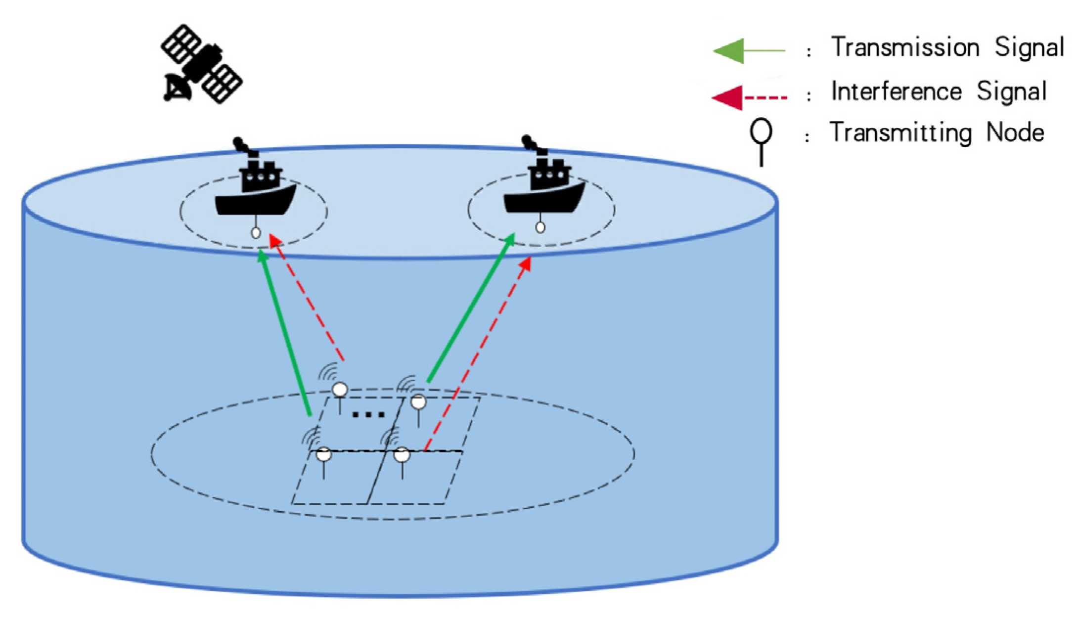
18]. Inspired by these works, we proposed a power allocation algorithm based on MADDPG for UACNs in this paper, because the multiple underwater nodes generate high-dimensional action and state space, and the collaboration of nodes has the advantage in learning. We take the transmitter nodes as agents and multiple agents can cooperate and share information for network training. Accordingly, we propose to maximize the channel capacity as the objective function, with the constraints of maximum power and minimum channel capacity. We model the power allocation problem as a Markov decision process (MDP) and apply the MADDPG approach to optimize power allocation. The actor and critic network of DDPG is trained using a central trainer, and its parameters are broadcast to multiple agents. Each agent updates its own actor network and inputs state to obtain actions for execution. This centralized training and distributed execution (CTDE) method iteratively trains the neural network until convergence to obtain a power allocation strategy. The main contributions of this study are as follows.
We propose a MADDPG-based power allocation scheme for UACNs. A MDP model is formulated and then the MADDPG is used to solve it. To the best of our knowledge, we first study using the MADDPG approach to solve the power allocation problem in UACNs. Although the MADDPG structure comes from [
15], we define the action, state, observation space, and reward function according to the objective function, and thus the MADDPG can be applied to the underwater network power allocation problem.
The consideration of the history information of CSI in the MDP model makes the proposed algorithm applicable to the underwater network involving mobility. Through the CTDE process, the multiple agents are trained collaboratively and make power allocation decisions adaptively to adapt to the changing underwater environment. Our approach is therefore better suited to underwater channels that vary due to fading and node movement.
The MDP model proposed in this paper can provide more QoS requirements in design. In the study, we guarantee QoS by requiring a minimum channel capacity. However, other QoS metrics, such as throughput, delay, or success transmission rate, can also be combined into the objective function. As a result, the MDP model can be adjusted to meet these QoS requirements and the MADDPG structure is still valid in these cases.
Simulation results show the total channel capacity of the proposed MADDPG power allocation performs better than that of DQN-based [
19] and DDPG-based [
13] algorithms with independent agent training. Also, the proposed method has a much lower running time compared with the FP algorithm, particularly with large networks.
3. Reinforcement Learning
3.1. Introduction to Actor–Critic
In RL, the agent interacts with the environment and learns the optimal policy to maximize the expected total reward over a time horizon. At time slot
, the agent takes action
in state
, where
and
represent action space and state space, respectively. After that, the environmental feedbacks reward
to the agent, and then the agent moves to the next state
. It then forms a sample of experience
) and stores it into replay memory
. The agent trains the neural network to maximize the discounted future reward when it obtains enough experience samples and then obtains optimal decision strategy. The discounted future reward
is defined as [
22]:
where
is a discount factor.
The policy updates include the value function-based method and the policy gradient-based method. The actor–critic framework combines these two methods. As shown in
Figure 2, the AC network consists of an actor neural network and a critic neural network, with network parameters
and
, respectively. Considering continuous action and state space, we exploit DDPG to solve our objective function; therefore, the actor network updates
using the deterministic policy gradient
, while the critic updates
using the gradient of the loss function.
The actor and critic are defined as follows:
Actor: The actor network updates policy
, which maps state space
into action space
, which is denoted by
According to policy
, the actor selects the action by the following rules:
where
is a random process.
Critic: The critic network estimates the action value
. It evaluates the new state by the temporal difference (TD) error, which is
The action selection weight will be enhanced if the TD error is positive. Otherwise, it is decreased with a negative TD error. The critic network and actor network parameters are updated as follows:
(1) Updates:
μ AC uses replay buffer
to store empirical samples
. The critic network randomly selects
mini-batch samples
for network training, and updates the parameters by minimizing the mean-squared loss function between the target Q-value and the estimated Q-value. The loss function is formulated by [
13]:
where
denotes the Q-value calculated by the target network and
is the step size of the iterative update. The target network with parameter
is used to maintain the stability of the Q-value, where
is updated periodically by
as
where
is used to slowly update the target network.
(2) Update
: The actor network is performed by a deterministic strategy, whose parameters are also trained from randomly selected samples. The goal of the actor is to find strategies that maximize the average long-term reward. The network parameters
are updated by [
13]:
where
is the step size of an iterative update to ensure that the critic is updated faster than the actor. The operation
represents gradient descent for functions. Similar to the critic network, the t update for the actor target network parameter
is
where
is used to update the target network.
3.2. MADDPG
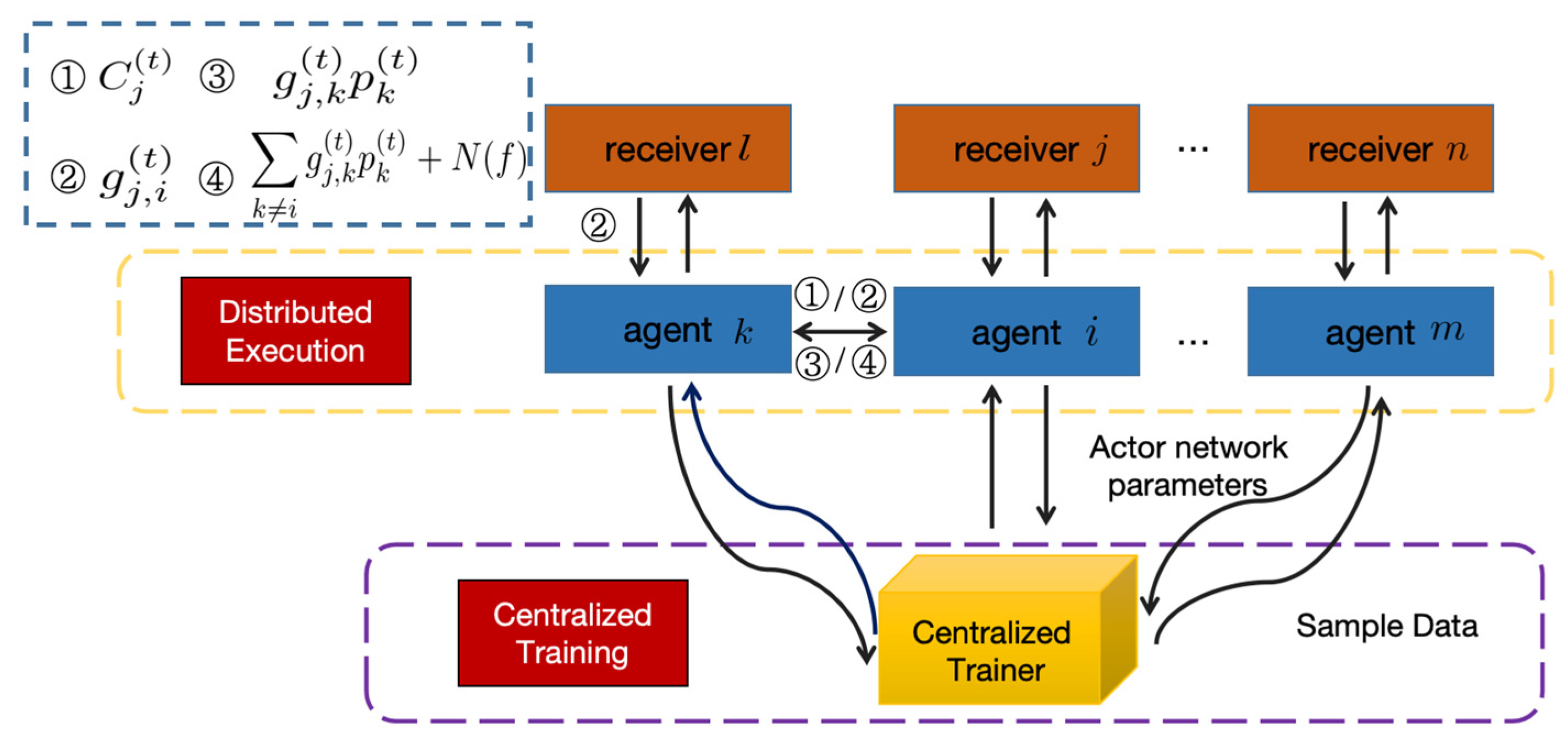
The UACNs environment contains multiple nodes. It is more efficient to use multi-agent reinforcement learning like MADDPG than DDPG with independent training by a single agent. However, training multiple agents leads to instability and invalid experience replay. To address these challenges, MADDPG utilizes a centralized training and decentralized execution (CTDE) framework, where a central trainer handles the learning process using the DDPG and broadcasts the training parameters to each agent. The central trainer includes the actor network, target actor network, critic network, and target critic network. The single agent only contains an independent actor network, whose parameters come from the central trainer. The single agent inputs the state to its actor network and obtains the action. This separation of training and execution allows more stable and efficient multi-agent learning. Each agent benefits from the shared learning while acting independently during execution.
There are agents in the UACNs, and for the agent , the parameters of the actor network and its local policy are denoted by and respectively. Therefore, the network parameters related to agents are described by and . The learning processes of multiple agents can be represented by a MDP model, which is defined by the state , action , observation and state transfer function . Agent uses the deterministic policy for action selection and moves to the next state according to the state transition function . It then receives the reward and also obtains the observation .
The central trainer updates the parameters of the critic network by minimizing the loss function [
15]:
where
is the Q-value of the target network, and
is the set of target policies, which is updated by Equation (16).
The actor network of agent
performs parameter updates by the gradient descent algorithm with the deterministic policy
. The loss function is [
15]:
where the replay buffer
stores samples from
agents at each time slot, which are
. After the training in the central trainer, the parameters of the
ith actor network are broadcasted to each agent. Each agent then uses the received parameters to independently update the actor network.
5. Simulation Results
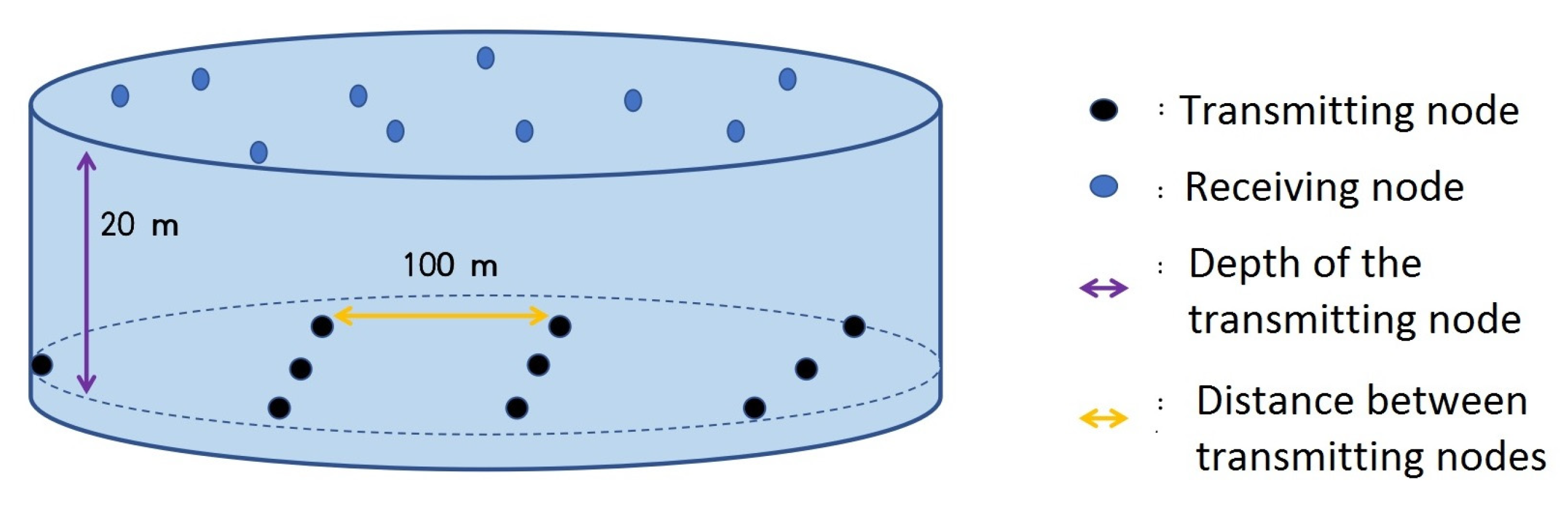
In this section, we evaluate the performance of the proposed MADDPG power allocation through simulations. We assume that
, and all source nodes are deployed underwater, as shown in
Figure 4. The source nodes are located
underwater with
between adjacent nodes. The receivers are on the water surface, with communication distances of
from the source nodes. The simulation parameters of the underwater acoustic environment are shown in
Table 1, where the wind speed, salinity, pH, temperature, and sound speed data are measured from the Yellow Sea of China in 2015 [
23]. We also assume the underwater acoustic channel is slow time varying and quasi-static flat fading, which means
is constant within a time slot.
According to [
24], the underwater sensor nodes are anchored and restricted by a cable, which can float in water. The nodes move at a speed of 0.83–1.67 m/s within the limit of the cable length [
24]. We adopt a moving speed of 0.9 m/s in the simulation. Therefore, the maximum Doppler frequency is 12 Hz. To avoid the space–time uncertainty caused by the long propagation delay of underwater acoustic transmission, we assume that the time slot length is long enough to complete information exchange and power allocation in the same time slot. Based on transmission distance and sound velocity, the time slot is assumed to be 2 s.
We compared the proposed MADDPG algorithm with fractional programming (FP) power allocation algorithm [
5], DQN training-based power allocation algorithm [
19], DDPG algorithm without collaboration [
13], random power allocation, and maximum transmitting power (full power).
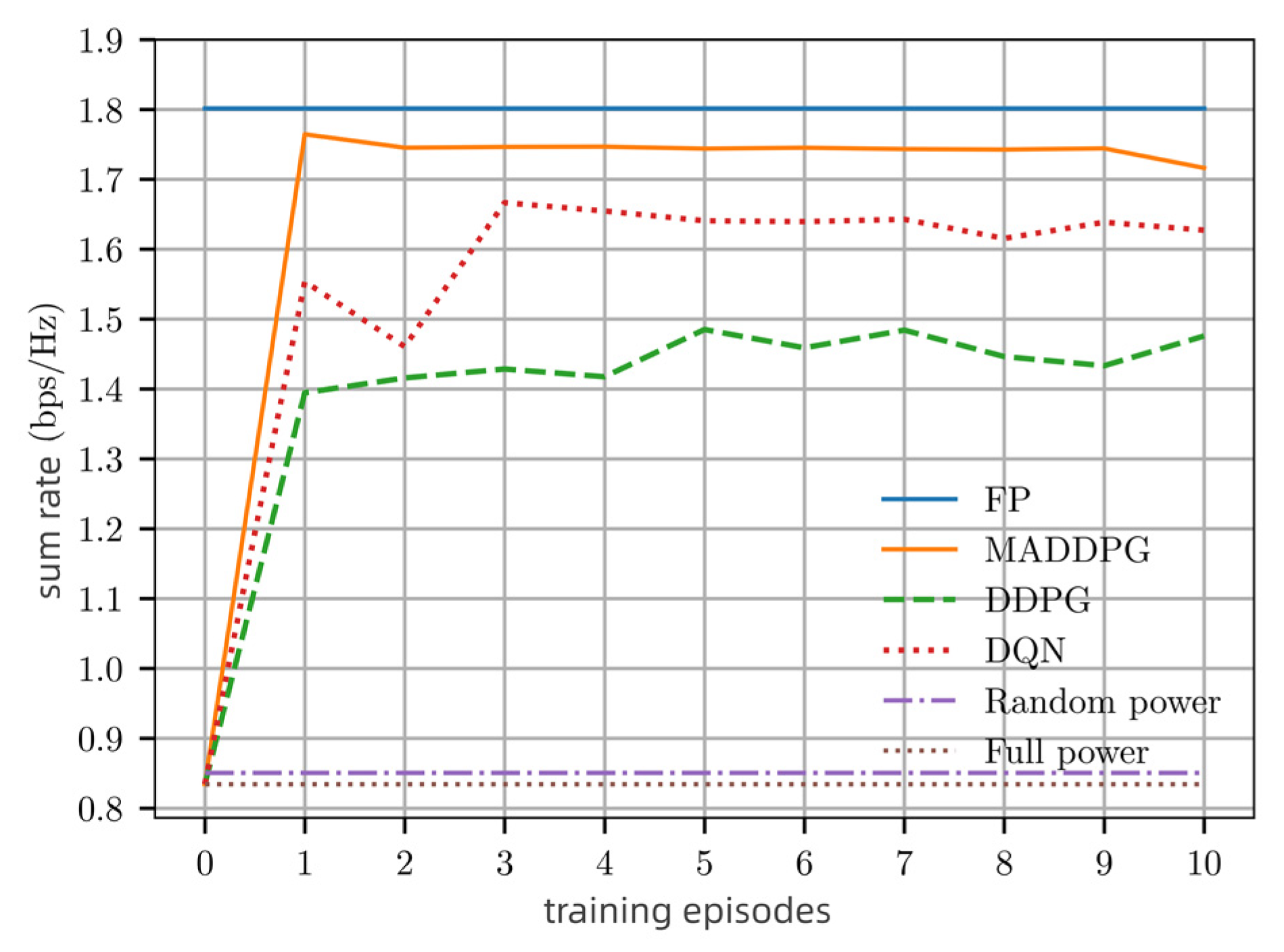
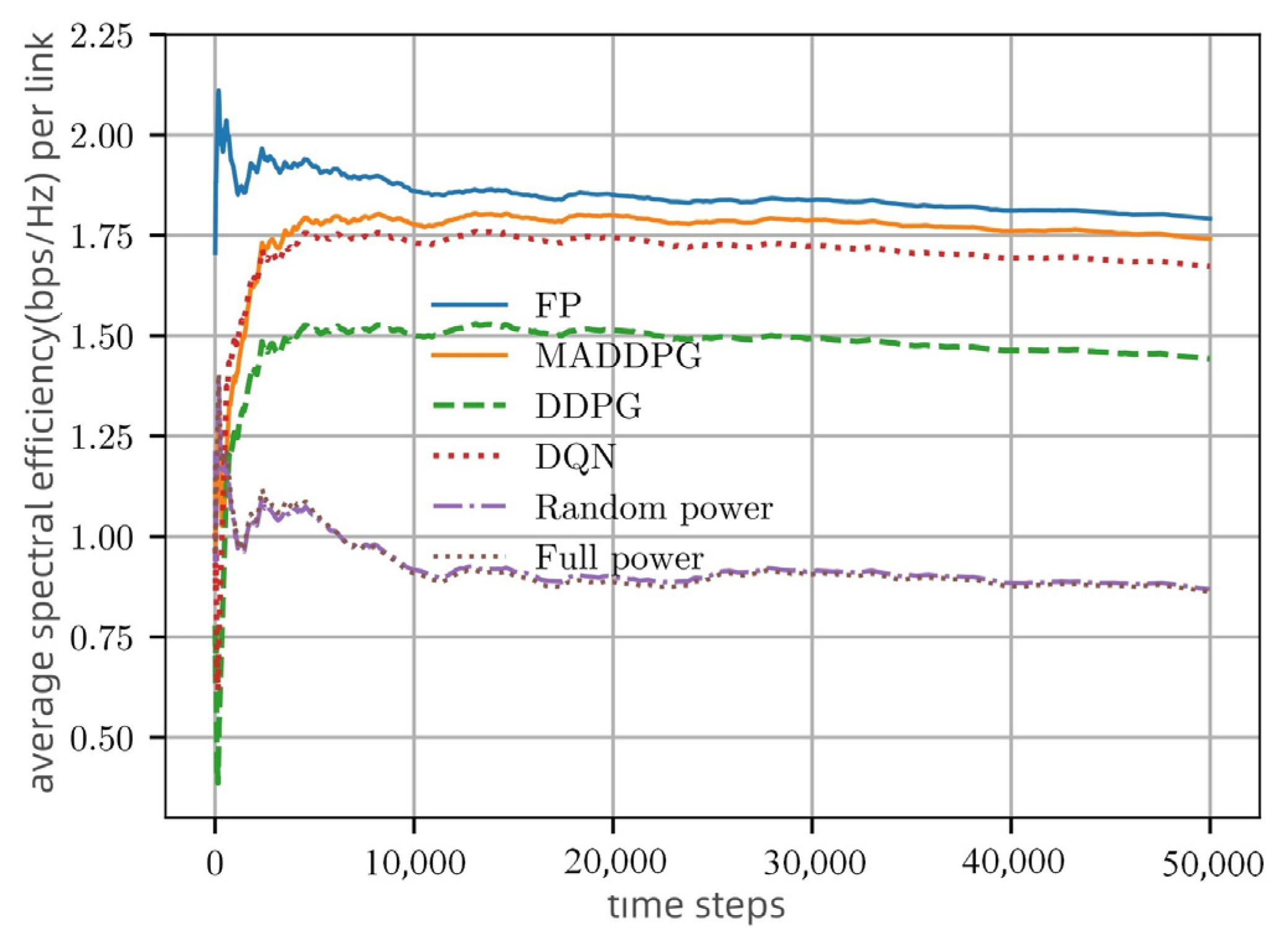
Figure 5 shows that the proposed MADDPG algorithm obtains a better sum rate compared with other power allocation strategies. The sum rate here refers to the sum channel capacity of all links. The sum rate of the proposed MADDPG power allocation remains above
, in which the
means bits per second. The FP algorithm is a model-driven method and has full CSI, whereas the deep learning methods such as DQN, DDPG, and MADDPG are only data driven without full CSI, resulting in lower performance than the FP algorithm. In the DQN and DDPG algorithms, each single agent is trained independently without interacting with the surrounding environment. However, the agents in MADDPG interact with each other and can use global data for centralized training, which obtains a better performance than DQN and DDPG. Random power and full power do not optimize power allocation, thus resulting in the worst performance.
Figure 6 compares the spectral efficiency (SE) performance of different algorithms in single-episode training. It can be seen that the SE of MADDPG is close to FP and outperforms other algorithms. Moreover, the MADDPG power allocation obtains convergence within 5000 training time steps, which has the same convergence rate as DQN.
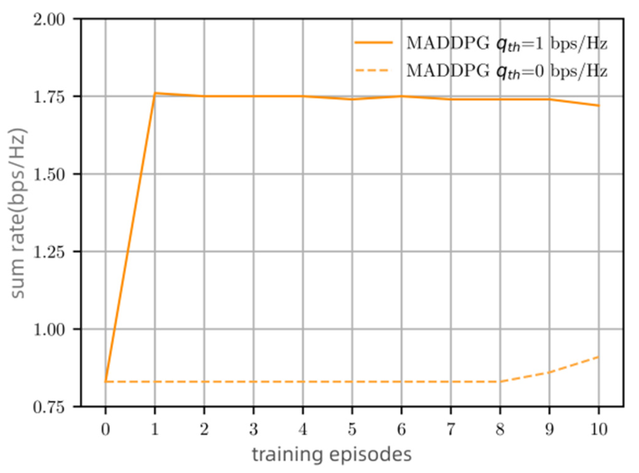
In the objective function
, the threshold
is required to ensure the minimum channel capacity of each link.
Figure 7 compares the sum rate of MADDPG power allocation with (
) and without (
) minimum channel capacity constraint. The algorithm considering
maintains a channel capacity of approximately 1.75 bps/Hz which performs 75% higher than that of without considering minimum channel capacity. Therefore, considering the minimum channel capacity constraint and penalty for interference in the reward function of our algorithm, each link can ensure a minimum channel capacity, which improves the system sum rate.
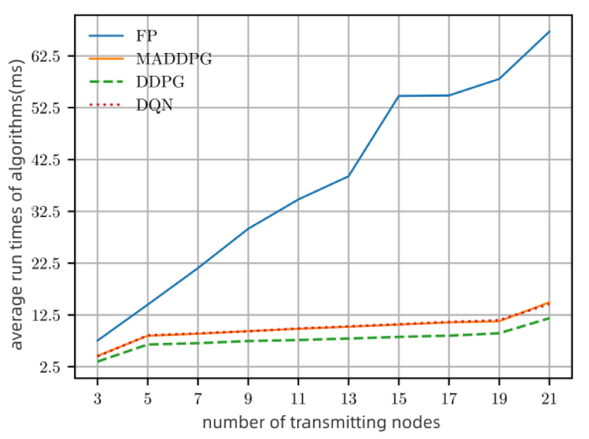
Figure 8 compares the computational complexity of different algorithms as the number of network nodes increases. We use the program running time to complete one-time power allocation as a metric. From
Figure 8, we can see that the number of nodes affects the complexity of the algorithm. The algorithms of MADDPG, DQN, and DDPG have approximately the same complexity, while FP is much higher. The per-iteration complexity of FP is
), while the others are
or less. Note that random and maximum power allocation algorithms are excluded from
Figure 8 since they do not need additional calculations.


