Learning Underwater Intervention Skills Based on Dynamic Movement Primitives

Abstract

Improving the autonomy of underwater interventions by remotely operated vehicles (ROVs) can help mitigate the impact of communication delays on operational efficiency. Currently, underwater interventions for ROVs usually rely on real-time teleoperation or preprogramming by operators, which is not only time-consuming and increases the cognitive burden on operators but also requires extensive specialized programming. Instead, this paper uses the intuitive learning from demonstrations (LfD) approach that uses operator demonstrations as inputs and models the trajectory characteristics of the task through the dynamic movement primitive (DMP) approach for task reproduction as well as the generalization of knowledge to new environments. Unlike existing applications of DMP-based robot trajectory learning methods, we propose the underwater DMP (UDMP) method to address the problem that the complexity and stochasticity of underwater operational environments (e.g., current perturbations and floating operations) diminish the representativeness of the demonstrated trajectories. First, the Gaussian mixture model (GMM) and Gaussian mixture regression (GMR) are used for feature extraction of multiple demonstration trajectories to obtain typical trajectories as inputs to the DMP method. The UDMP method is more suitable for the LfD of underwater interventions than the method that directly learns the nonlinear terms of the DMP. In addition, we improve the commonly used homomorphic-based teleoperation mode to heteromorphic mode, which allows the operator to focus more on the end-operation task. Finally, the effectiveness of the developed method is verified by simulation experiments.

1. Introduction

In the late 1970s, remotely operated vehicles (ROVs) became the main tool for underwater interventions, and operators located on the mother ship or shore base remotely operated the ROV to accomplish underwater interventions such as sampling, operating valves, welding, etc. [1,2]. The joystick currently used to control the underwater manipulator and the underwater manipulator has the same configuration of degrees of freedom, similar shapes, and proportional sizes, and the operator remotely operates the underwater manipulator directly in the joint space by referring to the underwater video of the feedback, while the ROV adopts a handle for remote operation [3]. This model has very high cognitive requirements for the operator, especially during delicate operations [4]. Additionally, as ocean exploration moves toward deeper and longer-term operations, the concept of resident ROVs has been introduced to reduce personnel and costs at sea by changing communication links [5,6]. However, the long-distance transmission of signals and bandwidth limitations add latency to the underwater operating system, which may lead to duplicate or overcorrected commands from the operator, affecting the efficiency of underwater interventions.

Enhancing the autonomy of underwater interventions reduces the operator’s operational burden while also helping to mitigate the impact of communication latency on operational efficiency. In this model, the operator only needs to send out high-level commands, and the slave terminal receives the commands and performs the control tasks in its own circuits, separating the master and slave control circuits to solve the problems caused by the time delay. Underwater autonomous intervention has also been a hot research topic in the last decade, and some research projects have begun to demonstrate underwater autonomous intervention capabilities. The SAUVIM project [7] proposes the first underwater vehicle able to intervene autonomously on a floating pedestal, where the operator only needs to confirm that the seafloor recovery target is within the searchable area during the entire operation process. In the TRITON project [8], vision-based servoing completes automated docking with underwater panels with a priori knowledge, as well as valve attachment, rotation, and extraction motions for fixed bases, a process that uses a task prioritization framework to control the underwater vehicle and manipulator to complete the gripping task. The PANDORA project [9] aims to provide the underwater vehicle with the ability to be continuously autonomous, thereby reducing the frequency of requests for assistance from the mother ship. The project uses a learning by demonstration (LbD) approach to learn and reproduce the operation process, where a small number of operator demonstrations based on dynamic movement primitive (DMP) learning are used to generalize the learned task knowledge into a model, and a hybrid force/motion controller is used to perform the rotary valve task. To the best of our knowledge, this would be the first application of demonstration learning techniques for underwater interventions. In the DexROV project of the EU [10,11], the operator interacts with the real-time simulation environment through a wearable manipulator with force feedback to complete the task, and the remote underwater ROV receives simple high-level semantic commands to complete the task autonomously, which learns the representation of the task based on a parameterized hidden semi-Markov model (TP-HSMM).

Due to the dynamic conditions of the underwater environment (current disturbances, reduced visibility, etc.), realizing autonomous underwater interventions is a considerable challenge. In addition, different intervention tasks require a lot of programming work. LbD is one of the most direct and effective skill-learning methods and can be based on existing underwater teleoperation technology, which is believed to help accelerate the process of autonomy for underwater interventions.

Most robot behavioral actions are imitated by tracking at the trajectory level. For example, in an underwater operation task, the variation in the operation task is usually between the position of the underwater manipulator and the position of the operation target, while the essence of the task is the same. Therefore, in this paper, we apply the method of DMP-based demonstration learning to underwater intervention, and we propose an underwater DMP (UDMP) method to address the problem of underwater interference affecting the demonstration trajectories. First, the Gaussian mixture model and Gaussian mixture regression (GMM–GMR) are used for feature extraction of multiple demonstration trajectories and regression to obtain typical trajectories. Second, the DMP method is used to learn that typical trajectory. By learning typical trajectories, the DMP method can be used to reproduce or generalize already-learned trajectories. This approach is compared to the one used in [12], which learns the nonlinear terms of the DMP directly. Simulation experiments show the effectiveness of the proposed method for demonstration learning for underwater intervention.

The rest of this paper is organized as follows. Section 2 summarizes LbD-related work in the robotics community and illustrates the incompatibility of existing approaches for underwater intervention applications. Section 3 describes the ROV system used for the intervention task. Section 4 presents our proposed learning framework and the main content of the UDMP approach. Section 5 shows the validity of the proposed method through simulation and comparison experiments. Section 6 summarizes our work and provides our outlook for future research.

2. Related Work

Unstructured work environments increase the difficulty of applying pre-programmed methods. In contrast, LfD provides an efficient and intuitive way to transfer skills from humans to robots. Task-relevant prior knowledge is extracted from the demonstration, and no other prior knowledge or data are required, making it a simple and effective way to characterize the operator’s actions when completing underwater intervention.

So far, many LfD algorithms have been proposed, such as DMP [13], a stable estimator of dynamical systems (SEDS) [14], the hidden Markov model (HMM) [15], probabilistic movement primitives (ProMP) [16], kernelized movement primitives (KMP) [17], and so on. The DMP method is proposed in [13] for generalizing point-to-point and periodic motions by learning a single demonstration trajectory. The method uses a spring-damping model and a nonlinear term to ensure that the generalized trajectory converges to the target point when imitating the demonstrated skill. The SEDS method, proposed in [14], is based on the dynamic systems (DS) algorithm and uses a nonlinear solver to optimize the parameters of a multi-sample GMM to ensure that the system is globally asymptotically stable under a quadratic Lyapunov function. The KMP method was proposed in [17], which minimizes the Kullback–Leibler divergence between parameterized and sample trajectories and introduces a Kernel trick to obtain a non-parametric skill learning model. Due to its generalization, stability, and robustness properties, DMP has been widely used in robotics to encode and reproduce motor behaviors such as pouring water [18], painting [19], and obstacle avoidance [20]. The DMP method has been particularly applied in the collaborative domain [21] by fusing it with impedance information obtained from electromyography (EMG)-based methods for estimating the stiffness of human limbs. In [22], collaborative skills are extracted from a single human demonstration and learned through a Riemannian DMP, where the learning process is adapted online according to human preferences and ergonomics to accomplish a human–machine collaborative handling task. In this research, the position, orientation, and stiffness of human demonstrations are learned to enable the human-like variable impedance control of robots.

Existing research has focused on manipulators for land-based applications, which usually require only one demonstration for a task to represent the characteristics of the taught trajectory since its base is usually cemented to the world. In contrast, an underwater manipulator is usually fixed to an ROV in a floating operation, and the movement of the manipulator may affect the movement of the ROV, thus changing the position of the manipulator’s base coordinates. In addition, due to the current interference in the underwater environment, the operator needs to resist the motion error caused by the current interference between the ROV and the manipulator during the teleoperation demonstration, so the demonstration data usually have a different starting point and end point, which is different from land manipulator demonstration learning. Therefore, it is not feasible to directly apply the DMP method, which requires only one acquisition of a typical trajectory on land, directly to the demonstration learning of an underwater manipulator. Skill learning for underwater manipulators requires learning multiple sets of demonstrations to obtain more trajectory features, creating a “1 plus 1 is greater than 2” effect. Currently, methods based on DMP learning of multiple demonstrations simultaneously focus on estimating the nonlinear forcing term in the DMP model via GMM [12,23] or obtaining the weight of the forcing term by transforming the term into solving a linear problem [24]. Inspired by ProMP and KMP, we use the probabilistic method GMM–GMR to preprocess multiple sets of demonstration trajectories before applying the DMP method to ensure the convergence of the trajectories. The aim is to preserve the common features contained in the demonstration trajectories, which are important for underwater demonstration learning. To illustrate the infeasibility of migrating the approach for land manipulators directly to underwater, in this paper, we compare our approach with that proposed in [12].

3. ROV Teleoperation System

3.1. System Constitution

The underwater teleoperation system consists of four parts (Figure 1): an operation control center (OCC), a satellite, an ROV, and tasks.

OCC includes an operator and a six-degree-of-freedom joystick with force feedback (CLAF_mini) to capture the operator’s hand movements. The slave end is an ROV that is in direct contact with the underwater environment and consists of the main frame, buoyancy material, power propulsion system, control and energy system, lighting and camera system, positioning system, and a seven-function underwater manipulator [25].

Table 1. The specifications of the CLAF_mini and ROV system.

	Item	Value
ROV	Design depth	11,000 m
	Size (L × H × W)	2.3 m × 1.3 m × 1.5 m
	Mass	1470 kg
	Thrusters	7
Manipulator	Maximum reach	1.6 m
	Function	7
	Lift at full extension	20 kg
CLAF_mini	Workspace	0.2 m × 0.2 m × 0.13 m
	Force	8.5 N

shows the specifications of the CLAF_mini and ROV.

When the operator accomplishes the underwater intervention task, he expresses the will to move by controlling the movement of the end of the CLAF_mini. After the mapping algorithm unit maps the movement of the end of the CLAF_mini to the desired movement of the ROV, which is transmitted to the ROV via the communication link. While the ROV executes control commands, the ROV’s status information and the video information of the surrounding environment are fed back to the OCC through the communication link for the operator to use as a reference for the next action.

3.2. Mapping Algorithm

Different from the traditional teleoperation of ROVs in joint space, considering the operator’s operating habit, we adopt the scheme of motion mapping between the master and slave in Cartesian space. However, since the master and the slave are heterogeneous, and the shape and size of the workspace are not the same, we develop workspace mapping algorithms to extend the smaller workspace of the master to the larger workspace of the ROV and the underwater manipulator, while guaranteeing operation accuracy and efficiency.

For the motion of the ROV, we adopt a velocity-based motion mapping strategy, considering that it usually performs a wide range of underwater exploration tasks. The desired velocity of the ROV is as follows:

$$v_{rov\_cmd}=k_{rov}\left(p_{joystick\_now}-p_{joystick\_init}\right),$$

(1)

where $k_{rov}$ is the mapping gain coefficient, and $p_{joystick\_now}$ and $p_{joystick\_init}$ are the current end position of the joystick CLAF_mini and the initial position of the current control cycle, respectively. The desired position of the end of the underwater manipulator is as follows:

$$p_{arm\_cmd}=p_{arm\_now}+k_{arm}\left(p_{master\_now}-p_{master\_init}\right),$$

(2)

where $k_{arm}$ is the mapping gain coefficient, $p_{arm\_now}$ is the current position of the end of the underwater manipulator, and $p_{master\_now}$ and $p_{master\_init}$ are the current position of the end of the manipulator and the initial position of the current control cycle, respectively.

For the orientation of the ROV and the end of the underwater manipulator, we use a 1:1 mapping method to ensure the master–slave end orientation is consistent.

4. Methods

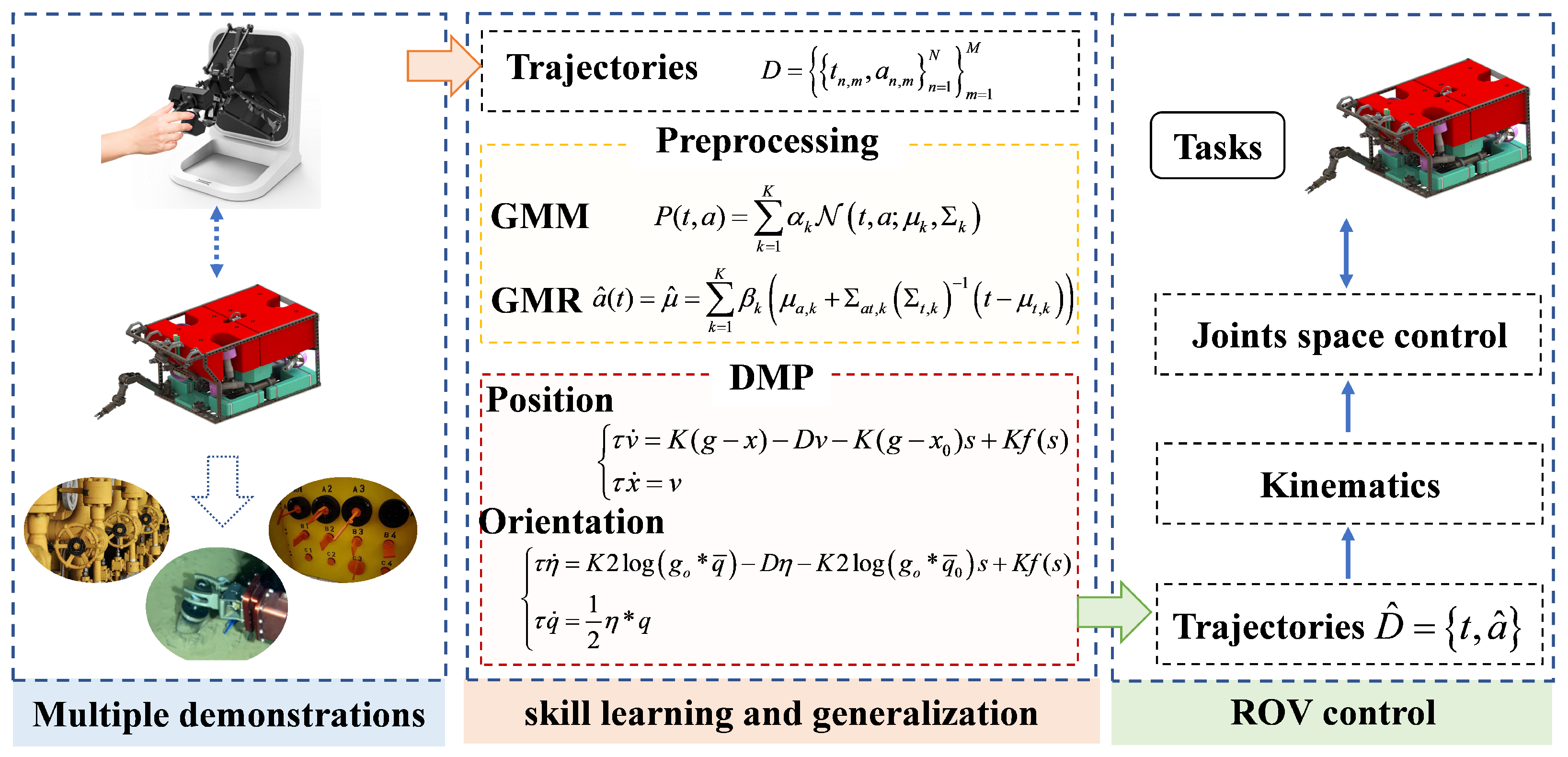
As shown in Figure 2, our learning framework consists of three main parts: multiple demonstrations, skill learning and generalization, and ROV control.

Multiple demonstrations: The operator remotely operates the ROV through the joystick to accomplish a task multiple times. The resulting demonstration trajectories are then aligned to the same time frame as the M demonstration trajectories. $D={\left\{{\left\{t_{n,m},a_{n,m}\right\}}_{n=1}^N\right\}}_{m=1}^M$ is the output of this module, $t_{n,m}$ denotes the demonstration time, $a_{n,m}$ denotes the position, orientation, velocity and acceleration of multiple trajectories, and N denotes the length of the sample data.

Skill learning and generalization: To address the problem that underwater environments (e.g., current perturbations and floating operations) attenuate the features of a single demonstration trajectory, we first encode multiple sets of multidimensional demonstration trajectories using GMM–GMR and generate typical trajectories $\widehat{a}\left(t\right)$ (position and orientation) that contain the operational features of an underwater intervention. Then, we use the extended DMP framework to model, learn, and generalize the typical trajectories of underwater interventions to obtain the desired trajectories $\widehat{D}=\{t,\widehat{a}\}$.

ROV control: The ROV receives the desired velocity command, and the underwater manipulator receives the desired end-effector position and orientation commands. The kinematics module is responsible for translating the end-effector position and orientation commands into the joint space, where the required control commands for each joint are computed by the underlying PID control.

4.1. GMM–GMR Preprocessing

To mitigate the influence of the underwater environment on the representativeness of the demonstration trajectories for underwater interventions, based on the assumption that each trajectory datum is composed of multiple Gaussian distributions, we use GMM–GMR to extract the features of multiple demonstration trajectories and fit the regression to produce a typical, smooth trajectory $\widehat{a}\left(t\right)$ that is characteristic of underwater interventions, so as to achieve the effect of one plus one is greater than two.

4.1.1. Gaussian Mixture Model

The joint probability density of a GMM is defined as follows [26]:

$$P(t,a)=\sum _{k=1}^K{\alpha }_k\mathcal{N}\left(t,a;{\mu }_k,{\Sigma }_k\right),$$

(3)

where ${\sum }_{k=1}^K{\alpha }_k=1$, and $\mathcal{N}$ is the Gaussian probability distribution defined as follows:

$$\mathcal{N}\left(t,a;{\mu }_k,{\Sigma }_k\right)={\displaystyle \frac{e^{-0.5{\left({[t,a]}^T-{\mu }_k\right)}^T{\Sigma }_k^{-1}\left({[t,a]}^T-{\mu }_k\right)}}{2\pi \sqrt{\left|{\Sigma }_k\right|}}},$$

(4)

where K is the number of Gaussian distributions, ${\alpha }_k$ is the weight, and ${\mu }_k$ and ${\Sigma }_k$ denote the mean and the covariance matrix of the kth Gaussian component, respectively.

To better represent the dataset without overfitting because of a large number of Gaussian components or underfitting because of a small number of Gaussian components, we use the Bayesian information criterion (BIC) to determine the number of Gaussian components [27]:

$$S_{BIC}=-L+{\displaystyle \frac{n\left(K\right)}{2}}lgN,$$

(5)

where $L={\sum }_{j=1}^{N}lg\left(p(t,a)\right)$ is the log-likelihood of the model using the demonstrations as a testing set, $n\left(K\right)$ is the number of free parameters required for a mixture of K components, and $n\left(K\right)=(K-1)+K(D+(1/2\left)D\right(D+1\left)\right)$. N is the number of D-dimensional datapoints. The value of K with the smallest value of $S_{BIC}$ is ultimately chosen to achieve a balance between the fit of the data and the number of parameters required.

The maximum expectation algorithm (EM) is used to estimate the GMM parameters, where the k-means algorithm is used to initialize the parameters ${\alpha }_k$, ${\mu }_k$, and ${\Sigma }_k$ to mitigate the sensitivity of the EM algorithm to the initial values [28]. The EM algorithm aims to find the parameters that maximize the log-likelihood function:

$${\widehat{\pi }}_k=\underset{{\pi }_k}{argmax}log\left(p\left(t,a\mid {\pi }_k\right)\right).$$

(6)

4.1.2. Gaussian Mixture Regression

We use time t as the query point and estimate the corresponding trajectory values $\widehat{a}$ via GMR regression [27]. The conditional probability density of a given t is as follows:

$$P(a\mid t)\sim \sum _{k=1}^K{\beta }_k\mathcal{N}\left({\widehat{\mu }}_k,{\widehat{\Sigma }}_k\right).$$

(7)

As a result, a smooth motion trajectory extracted from a plurality of demonstration trajectories containing operator demonstration features is represented as follows:

$$\widehat{a}\left(t\right)=\widehat{\mu }=\sum _{k=1}^K{\beta }_k\left({\mu }_{a,k}+{\Sigma }_{at,k}{\left({\Sigma }_{t,k}\right)}^{-1}\left(t-{\mu }_{t,k}\right)\right).$$

(8)

4.2. Cartesian Space Dynamic Movement Primitive

4.2.1. DMP for Position

We use a discrete DMP as the basic motion model, which consists of two parts: a stiffness damping system and a nonlinear forcing term [13], which can be expressed as follows:

$$\left\{\begin{array}{c}\tau \dot{v}=K_p(g-x)-D_{p}v+\left(g-x_0\right)f\left(s\right)\hfill \\ \tau \dot{x}=v\hfill \end{array},\right.$$

(9)

where $x,v\in \mathbb{R}$ are the position and velocity of the system at a certain moment, $x_0\in \mathbb{R}$ is the initial position of the system, and $g\in \mathbb{R}$ is the target position of the system. $K_p,D_p\in {\mathbb{R}}^{+}$ are the stiffness and damping term coefficients, respectively, and the system is critically damped when $D_p=2\sqrt{K_p}$. $\tau \in {\mathbb{R}}^{+}$ is the time-scaling coefficient, $f\left(s\right)$ is the forcing term, and $s\in (0,1]$ is a reparameterized representation of time $t\in [0,T]$, controlled by a regular system as follows:

$$\tau \dot{s}=-{\alpha }_{p}s,$$

(10)

where ${\alpha }_p\in {\mathbb{R}}^{+}$ is the exponential decay coefficient of the regular system with an initial value $s\left(0\right)=1$. The forcing term $f\left(s\right)$ is written as follows:

$$f\left(s\right)={\displaystyle \frac{{\sum }_{i=0}^N{\omega }_i{\psi }_i\left(s\right)}{{\sum }_{i=0}^N{\psi }_i\left(s\right)}}s,$$

(11)

where ${\psi }_i\left(s\right)=exp\left(-h_i{\left(s-c_i\right)}^2\right)$ is the Gaussian basis function (GBF) with center $c_i$ and width $h_i$. N is the number of Gaussian functions, and when the regular system converges to the target, the corresponding Gaussian functions are activated, and the forcing term takes effect.

The above DMP formulation suffers from the problem of cross-zeroing because of the coupling of the relative position between the target position and the start position with the forcing term, e.g., when the sign of the target position is changed, the learned trajectory is also mirrored. Therefore, to overcome the above drawbacks, we use the proposed extended DMP where the forcing term no longer relies on the relative position between the start and end points [29,30]:

$$\left\{\begin{array}{c}\tau \dot{v}=K_p(g-x)-D_{p}v-K_p\left(g-x_0\right)s+K_{p}f\left(s\right)\hfill \\ \tau \dot{x}=v\hfill \end{array}.\right.$$

(12)

The learning process focuses on calculating the weight $w_i\in \mathbb{R}$ that is closest to the desired forcing term, and we rewrite Equation as follows (12):

$$f_d\left(s\left(t\right)\right)=1/K_p\left(\tau \dot{v}-K_p(g-x)+D_{p}v+K_p\left(g-x_0\right)s\right).$$

(13)

Thus, the minimized loss function expression is as follows:

$$J_i=\sum _{t=1}^T{\psi }_i\left(t\right){\left(f_d\left(t\right)-w_i\xi \left(t\right)\right)}^2,$$

(14)

where $\xi \left(t\right)=s\left(t\right)$, and it can be obtained by solving the local weighted regression (LWR):

$$w_i={\displaystyle \frac{s^T{\psi }_i{f}_d}{s^T{\psi }_{i}s}}.$$

(15)

4.2.2. DMP for Orientation

Unlike the position, which can be decoupled into three separate one-dimensional motions, the set of orientations $\mathrm{SO}\left(3\right)$ is a three-dimensional manifold that does not allow for the decoupling scheme described above. In addition, in contrast to rotation matrices, we use the unit quaternion representation of the orientations because it provides a singularity-free, nonminimal representation of the orientations, where a logarithmic mapping function is used to compute the distance between two quaternions [31,32], and the conjugate of q is denoted by $\overline{q}=-u+v$:

$$d\left(q_1,q_2\right)=\left\{\begin{array}{cc}{[0,0,0]}^{\mathrm{T}},\hfill & q_1\ast {\overline{q}}_2=-1+{[0,0,0]}^{\mathrm{T}}\hfill \\ 2∥log\left(q_1\ast {\overline{q}}_2\right)∥,\hfill & \mathrm{otherwise}\hfill \end{array}\right..$$

(16)

The quaternion logarithm log, $S^3\mapsto {\mathbb{R}}^3$, is defined as follows:

$$log\left(q\right)=log(v+u)=\left\{\begin{array}{c}arccos\left(v\right){\displaystyle \frac{u}{\parallel u\parallel }},u\ne 0\hfill \\ {[0,0,0]}^{\mathrm{T}},\mathrm{otherwise}\hfill \end{array}.\right.$$

(17)

Therefore, the DMP model of orientation can be expressed as follows:

$$\left\{\begin{array}{c}\tau \dot{\eta }=K_{o}2log\left(g_o\ast \overline{q}\right)-D_o\eta -K_{o}2log\left(g_o\ast {\overline{q}}_0\right)s+K_{o}f\left(s\right)\hfill \\ \tau \dot{q}={\displaystyle \frac{1}{2}}\eta \ast q\hfill \end{array}.\right.$$

(18)

The relation between the quaternion derivative and angular velocity is given by $\dot{q}={\displaystyle \frac{1}{2}}\omega \ast q$; we obtain $\eta =\tau \omega$, and $\omega =2log\left(q_1\ast {\overline{q}}_2\right)/\mathrm{d}t$. Integrating the quaternionic derivative yields the following:

$$q(t+\Delta t)=exp\left({\displaystyle \frac{\Delta t}{2}}{\displaystyle \frac{\eta \left(t\right)}{\tau }}\right)\ast q\left(t\right),$$

(19)

where the exponential mapping of quaternions ${\mathbb{R}}^3\mapsto S^3$ is defined as follows:

$$exp\left(r\right)=\left\{\begin{array}{c}cos(\parallel r\parallel )+sin(\parallel r\parallel ){\displaystyle \frac{r}{\parallel r\parallel }},r\ne 0\hfill \\ {[0,0,0]}^{\mathrm{T}}+1,\mathrm{otherwise}\hfill \end{array}.\right.$$

(20)

5. Simulation

The simulation environment is the ROV simulation environment built in the previous study [25]. In this simulation environment, the ROV has basic video feedback and dynamic positioning capabilities, and the underwater manipulator has basic functions such as teleoperation and joint space PID control. The experiment is run under the Ubuntu 18 operating system, and Figure 3 shows the composition of the experimental system. The experimental conditions were set as follows: the ROV was dynamically positioned at a depth of 95 m, and the fluid density was set to 1028 kg/m³.

To evaluate the performance of our method for learning from demonstrations for underwater interventions, we compare it to the method in [12], which is an effective method for solving the problem of learning from multiple demonstrations, except for its application to robots on land. The approach in this paper we refer to as UDMP, and the approach in [12], which we refer to as DMP.

5.1. Collection of Multiple Demonstration Trajectories

In this experiment, we assume that the ROV has sailed to the vicinity of the operational target, and the operator remotely operates the manipulator after turning on dynamic positioning. We collect six trajectories when the operator completes the valve-gripping task, the initial state of the ROV is similar in each trajectory, and the operator completes the underwater intervention task based on the feedback video. 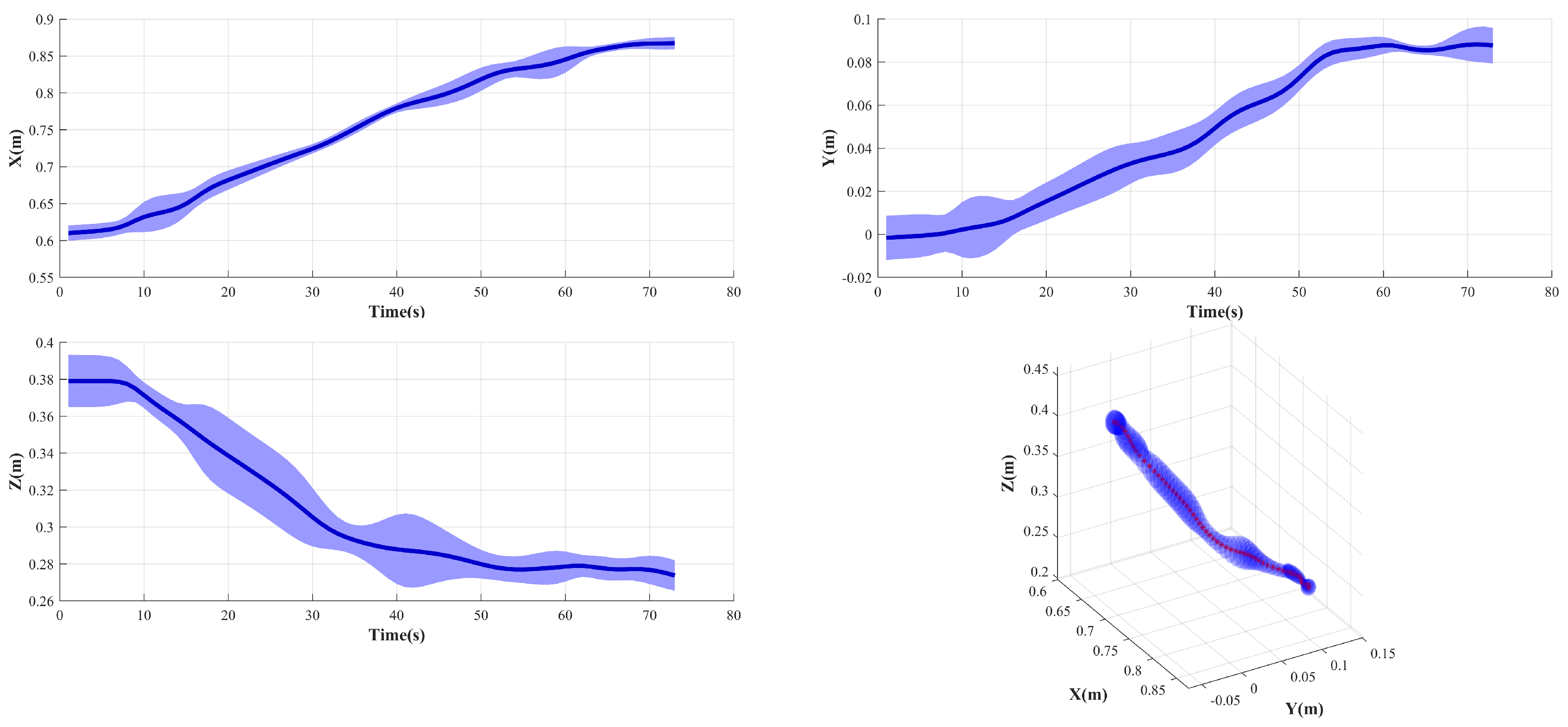Figure 4 shows the position of the demonstration trajectories. 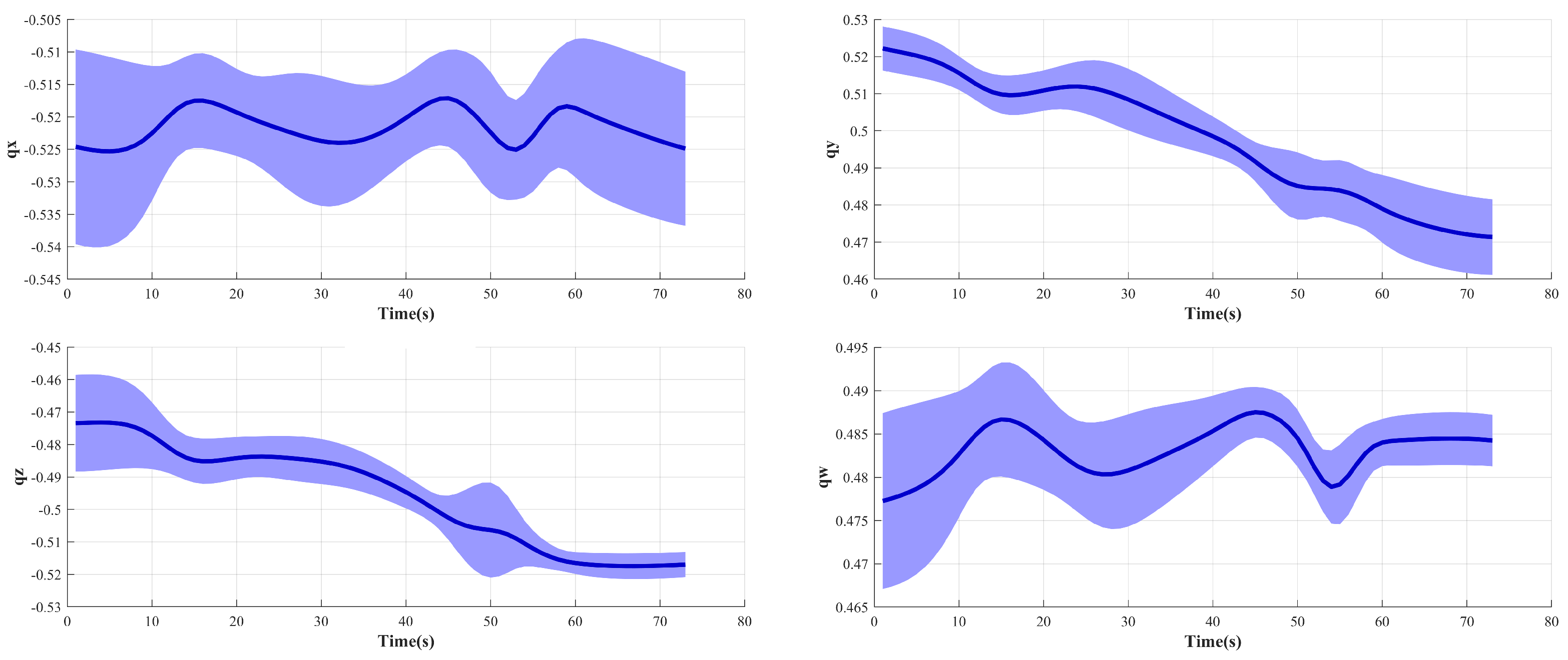Figure 5 shows the orientation of the demonstration trajectories.

The figure shows that the collected trajectories are not smooth, which is due to the fact that underwater intervention tasks are different from land operation tasks. First, the ROV operator can only use the video feedback from a limited number of cameras on the ROV as a reference during teleoperation, while most of the applications on land have global information feedback. Second, due to the effects of current disturbances and dynamic positioning errors on the ROV’s position, the ROV operator needs to continuously adjust the position and orientation during teleoperation to mitigate the effects of the floating base, whereas most applications on land are based on a fixed base.

5.2. Learning from Multiple Demonstrations

Since the durations of multiple presentations may be different, we regularized the time of the trajectory set at the same time, after which we used GMM–GMR for operational task feature extraction as well as regression fitting, as shown in Figure 6 and Figure 7. The Gaussian component of the position trajectories obtained using the BCI rule is 14, and the Gaussian component of the orientation trajectories is 11.

The results indicate that the variance (the width of the blue band) becomes progressively smaller as we approach the valve, indicating that the constraints become progressively stronger due to the same target position and orientation for each demonstration. The trajectory variance is larger in the initial stage due to the disturbance caused by the current to the ROV, which makes the initial position and orientation different. The dark blue curve in the figure indicates the trajectory with typical characteristics obtained after GMM–GMR preprocessing, which contains the trajectory characteristics of underwater intervention.

The method in [12] is used to learn and regress the nonlinear term $f\left(s\right)$ of the DMP model directly using GMM–GMR. Figure 8 and Figure 9 show the relationship between s and $f\left(s\right)$ that we obtained using this method. The Gaussian component of the position trajectories obtained using the BCI rule is 4, and the Gaussian component of the orientation trajectories is 8. It can be observed that the width of the blue band representing the variance of the forcing term $f\left(s\right)$ first becomes narrower and then wider and then narrower. This is consistent with the actual operation process, in which the position and orientation of the end of the underwater manipulator must satisfy the operational requirements of the initial and final moments, i.e., the constraints are strong, while the constraints of the intermediate processes are weak.

5.3. Replication and Generalization of Skill

The purpose of this subsection is to validate the effectiveness of the UDMP method proposed in this paper for underwater intervention demonstration learning, as well as to compare it with the DMP method in [12].

The UDMP requires the tuning of three parameters to accommodate different trajectory behaviors, including the number of Gaussian functions of the nonlinear terms N, the spring factor K, and the attenuation coefficient $\alpha$. The DMP requires the tuning of two parameters to accommodate different trajectory behaviors, including the spring factor K and the attenuation coefficient $\alpha$. A higher K causes the system to respond to the target trajectory more quickly but may cause oscillations. A higher $\alpha$ makes the system converge to the target quickly. To ensure the smoothness and robustness of the learned trajectories, the parameter settings for this experiment are shown in

Table 2. The parameter settings for DMP and UDMP.

	Position			Orientation
	${\mathit{\alpha }}_{\mathit{p}}$	${\mathit{K}}_{\mathit{p}}$	${\mathit{N}}_{\mathit{p}}$	${\mathit{\alpha }}_{\mathit{p}}$	${\mathit{K}}_{\mathit{p}}$	${\mathit{N}}_{\mathit{p}}$
DMP	0.05	0.25		1	900
UDMP	0.05	0.25	50	1	900	50

.

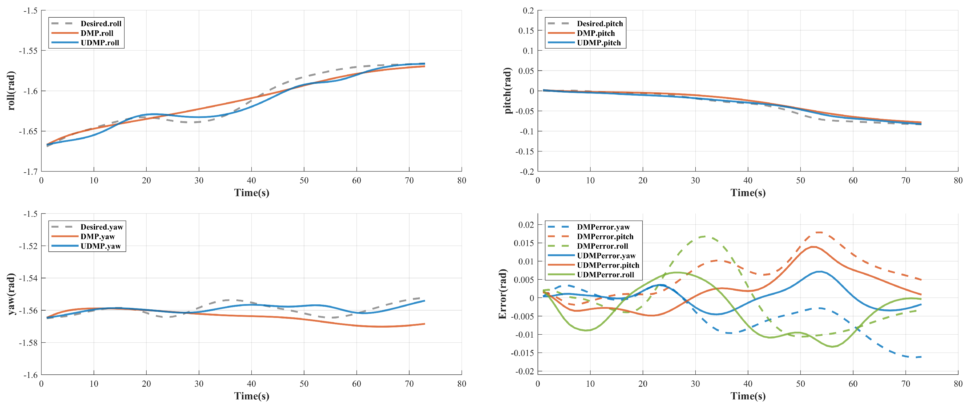
We used the DMP and UDMP methods for demonstration reproduction, respectively, and the reproduction results for position and orientation are shown in Figure 10 and Figure 11. The reproduction results of the two methods are shown in

Table 3. Errors in demonstration replication using DMP and UDMP methods.

		Position			Orientation
		x (m)	y (m)	z (m)	Roll (rad)	Pitch (rad)	Yaw (rad)
DMP	rmse	0.0037	0.0024	0.0026	0.0073	0.0084	0.0081
	max. error	0.0099	0.0053	0.0066	0.0162	0.0178	0.0168
UDMP	rmse	0.0016	0.0007	0.0007	0.003	0.0057	0.0072
	max. error	0.0043	0.0021	0.0023	0.0072	0.0139	0.0134

. From the results, it can be observed that the errors of both methods tend to be zero, but compared to the DMP method, UDMP learns better for the features of underwater interventions, especially in the orientation dimension, and UDMP can learn better from the demonstrative data which has little change in orientation.

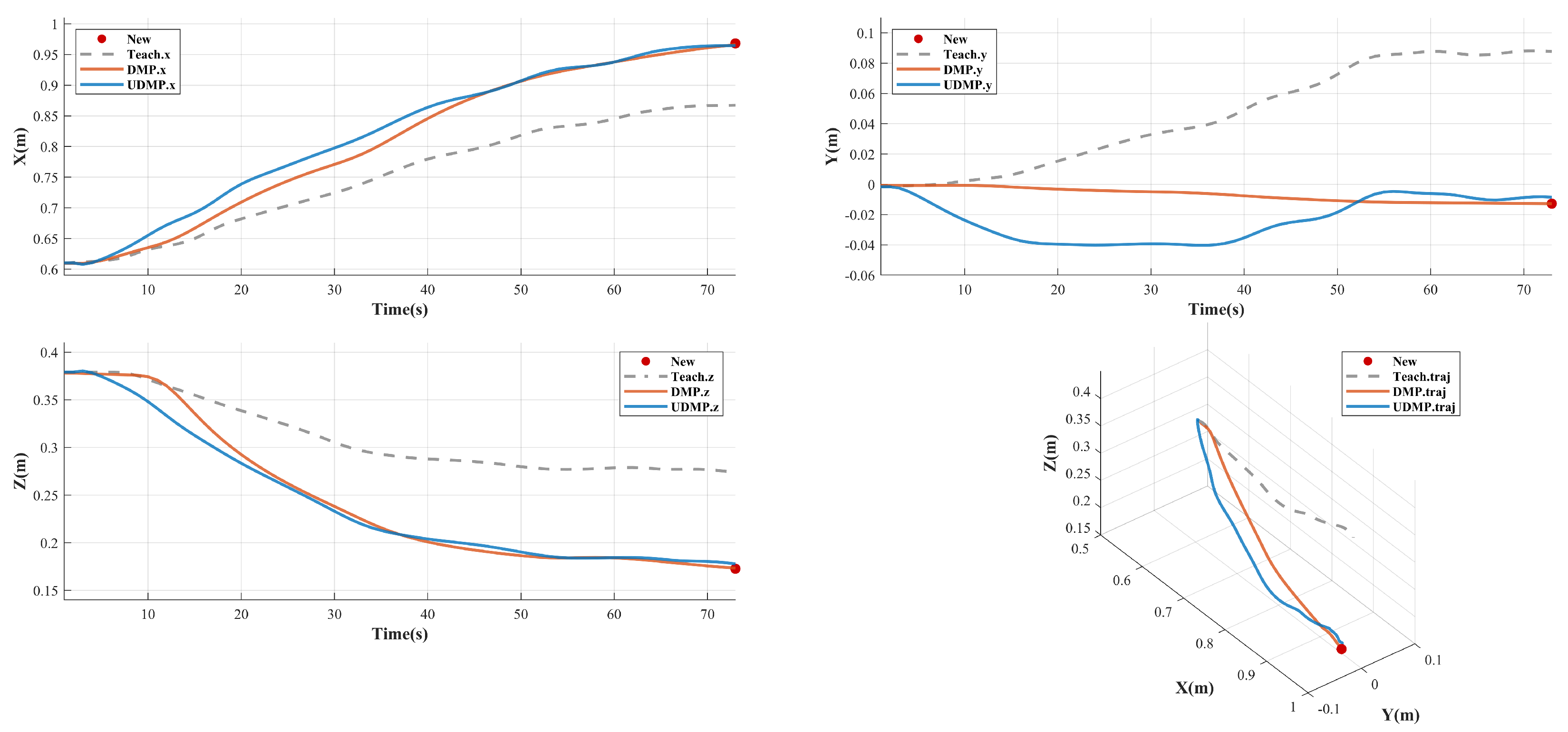
To further validate the learning performance of the UDMP method, we changed the position of the valve so that it could be approached without changing the orientation. This is due to the fact that the valve position, i.e., the target position, is usually changed in this type of underwater intervention task, and the orientation of the underwater manipulator end-effector when approaching the valve is usually the orientation facing the valve, i.e., it is similar to the initial orientation of the manipulator end-effector in this experiment. Still, using the parameters in Table 2, the results after the generalization of the new position using the DMP method and the UDMP method are shown in Figure 12. The trajectories obtained from the generalization of both methods converge to the desired new target position, and the generalization result of the proposed UDMP method is similar to the shape of the demonstration trajectory, i.e., the constraints in the motion process guarantee the phase, while the DMP method is different from the shape of the demonstration trajectory. Although all of them eventually converge to the target position, the learning of the shape of the trajectory is the focus of this paper’s research, so the above results show that the UDMP method proposed in this paper is effective for the application of underwater intervention demonstration learning.

6. Conclusions

To mitigate the effects of communication delays on underwater intervention tasks as well as to reduce the cognitive burden on the operator, this paper adopts an intuitive LfD approach to learn operational skills from a small number of demonstrations, thereby enhancing the autonomy of underwater intervention. To address the problem that the complexity and randomness of the underwater operation environment (e.g., current disturbance and floating operation) diminish the representativeness of the demonstration trajectories, we propose the UDMP method, in which multiple demonstration trajectories are feature-extracted using GMM–GMR, a typical trajectory is obtained, and then, the trajectory is modeled using the DMP method. Experiments show that the proposed UDMP method can extract more motion features than the existing methods that learn the nonlinear terms of DMP. This is due to the fact that demonstration trajectories of underwater intervention are noisy, and the DMP method that learns the nonlinear term indirectly will lose some trajectory features, while the proposed UDMP method directly extracts the features of the taught trajectory first and then proceeds to the learning of the DMP model to retain more motion features, which is exactly what is required for the learning of demonstration trajectories of underwater intervention.

The underwater intervention in this paper does not consider operational tasks that require contact force. In future work, we will consider learning the contact force during underwater intervention as a way to adapt to more operational tasks.