Abstract
Moving target defense (MTD) technology baffles potential attacks by dynamically changing the software in use and/or its configuration while maintaining the application’s running states. But it incurs a deployment cost and various performance overheads, degrading performance. An attack graph is capable of evaluating the balance between the effectiveness and cost of an MTD deployment. In this study, we consider a network scenario in which each node in the attack graph can deploy MTD technology. We aim to achieve MTD deployment effectiveness optimization (MTD-DO) in terms of minimizing the network security loss under a limited budget. The existing related works either considered only a single node for deploying an MTD or they ignored the deployment cost. We first establish a non-linear MTD-DO formulation. Then, two deep reinforcement learning-based algorithms are developed, namely, deep Q-learning (DQN) and proximal policy optimization (PPO). Moreover, two metrics are defined in order to effectively evaluate MTD-DO algorithms with varying network scales and budgets. The experimental results indicate that both PPO- and DQN-based algorithms perform better than Q-learning-based and random algorithms. The DQN-based algorithm converges more quickly and performs, in terms of reward, marginally better than the PPO-based algorithm.
1. Introduction
Moving target defense (MTD) [1,2] is a kind of proactive defense technique, which makes the adversary face a random and ever-changing view of the underlying software. Therefore, there is an increase in the difficulty of successful exploits and the required effort, deterring the adversary from further attacks. It is reported that over 5000 companies have deployed MTD technology in approximately nine million endpoints and Windows and Linux servers [3]. However, the problem of maintaining its defense effectiveness in budget-constrained environments is not trivial. MTD techniques may incur deployment costs and various overheads, degrading their performance. Hence, it is highly challenging to identify an optimal setting in which to deploy the MTD and then maximize its defense effectiveness (e.g., minimizing attack success) under a limited budget.
The attack graph technique has been applied for analyzing passive [4] and proactive [5] defense mechanisms in the literature. This study focuses on proactive mechanisms. An attack graph has been developed for designing an MTD deployment mechanism [5]. Similarly, the authors in [6] proposed a more effective MTD scheme for DDoS attacks. Deep reinforcement learning (DRL) is a technique used to solve sequential decision-making problems and, recently, its efficacy has been demonstrated in a variety of complex domains [7]. Also, studies have been conducted on applying deep reinforcement learning (DRL) for optimizing
MTD, like [8,9,10,11]. However, all these existing works only considered a single vulnerable node, which deploys the MTD technique.
This study explores the use of DRL and attack graph techniques to achieve MTD deployment effectiveness optimization (denoted as the MTD-DO problem) in network scenarios, where (i) there are a set of attacking nodes; (ii) MTD can be leveraged at any node; and (iii) there is a limited budget for deploying MTD. The authors in [12] studied the deployment of a redundancy-based MTD technique over a target network. They formulated a mixed-integer linear program formulation for minimizing the probability of successfully attacking without considering the MTD deployment cost. Different from [12], we consider the cost, and our problem is non-linear. Note that there are works applying MTD deployment optimizations based on DRL techniques (see [13] and the references therein), but they only consider a single vulnerable node.
There are various MTD implementation methods, like changing Internet protocol (IP) and medium access control (MAC) addresses or routing paths randomly, migrating VMs from one host to another and randomizing the data [1]. Each type of MTD implementation method uses several candidates to achieve its specific redundancy. Without a loss of generality, this study uses backup components to denote a candidate without considering its specific implementation, just for easy expression. Usually, the greater the number of backup components, the greater the cost. It is noticed that more backup components do not mean an improvement in security. By MTD deployment effectiveness, we mean how many backup components are deployed at each attack graph node, such that the security loss (defined in Equation (1) in Section 2) is within the limited budget. We aim to investigate which DRL techniques out of Q-learning [14], Deep Q-Learning (DQN) [14,15], and PPO [15,16] make for the most cost-effective defense in the aforementioned scenario. It is noticed that the problem considered in this study has a discrete action space; thus, traditional policy-based DRL algorithms for a continuous action space, like the Deep Deterministic Policy Gradient, cannot be directly adopted.
The main contributions of this study are listed as follows:
- (a)
- We create a mathematical formulation of the MTD-DO problem, which is a non-linear optimization problem. Different from existing works, we consider a network scenario where each node can apply an MTD strategy as long as the budget is large enough. Actually, our work can be directly applied to a scenario where some nodes cannot use an MTD by setting the value of the related node to zero, as defined in Section 3. To the best of our knowledge, we are the first to optimize MTD deployment in a scenario with more than one vulnerable node.
- (b)
- We propose two RL-based MTD-DO algorithms, namely, PPO-based and DQN-based algorithms, in our DRL approach. We detail them in Section 4. It is known that for reinforcement learning algorithms, the factors that mainly affect their problem-solving efficiency are the size of the action space and the state space. Assuming there are N nodes, the action space of the constructed MDP is N + 1, and the state space is 3N + 1. Both the action space and state space have a complexity of O(n), which means DRL has good scalability and can handle larger attack graphs with more nodes and connections.
- (c)
- We propose two metrics (see Equations (12) and (13)), which can effectively evaluate MTD-DO algorithms in varying network scale and budget.
The rest of this paper is organized as follows. Section 2 presents related work, and Section 3 describes the attack graph-based MTD deployment optimization problem. Section 4 gives our DRL approach, including the DQN- and PPO-based MTD-DO algorithms. We evaluate the proposed algorithms in Section 5. In Section 6, we summarize the work presented in this paper.
2. Background and Related Work
This section first focuses on the related works on improving the effectiveness of MTD techniques.
2.1. Background
2.1.1. Attack Graph
An attack graph [17] can graphically describe all the possible attacking routes through which an adversary can apply to reach their malicious goals. AG is one well-known solution for evaluating the security, by directly displaying the existence of vulnerabilities in the system and illustrating how the adversary can exploit these vulnerabilities to carry out an effective attack.
2.1.2. Moving Target Defense
MTD [18,19,20] is a paradigm, which aims to protect the computer and network in a proactive and adaptive approach. There are typically three types of techniques for implementing MTD, namely, shuffling, redundancy, and diversity. Shuffling tries to randomize and reorganize the system’s configuration so as to create uncertainty for the adversary and then confuse the adversary. Diversity exploits multiple implementations to reduce the attacking impact on the system security. Redundancy endeavors to maintain system reliability and stability by deploying entity (devices/applications/platforms) redundancies. The redundancy strategy has been widely deployed in SDN-based networks.
From the perspective of when to trigger MTD operation, there are usually the following three types of MTDs [18].
- (1)
- Time-based MTD: The MTD operation starts to work periodically. The interval of the two MTD operations is a controllable/adjustable parameter that can be decided by the security administrator.
- (2)
- Event-based MTD: When the detection of an attack is successful, the MTD operation starts to work in order to protest the target from the later potential attacks.
- (3)
- Hybrid MTD: It is a combination of time-based and event-based strategies to achieve a tradeoff among security level, service performance, the caused overheads, and so on.
2.2. Related Work
Since MTD was proposed, various techniques were applied for its effectiveness. Analytical modeling-based approaches [19,20,21] and measurement-based approaches [22] were proposed for evaluating MTD effectiveness. The first type cannot provide direct guidelines for MTD implementation optimization. State–space analytical modeling-based approaches can capture the time dependency relationship of the system elements. But there is a limitation for state–space analytical modeling in capturing the large-scale system. The attack graph technique is a non-state–space analytical modeling approach and can be used for large-scale systems. But it cannot capture the time dependency relationship among system elements.
Recently, various MTD-based methods have been proposed to defeat attacks like DDoS attacks. The authors [23,24] explored game-theory techniques to design optimized MTD implementation. The authors in [8,9,10,11] explored machine learning and deep reinforcement learning (DRL) for optimizing MTD. However, they considered only one vulnerable target. They fixed the number of MTD backup entities and determined when and which to transfer service to reduce the attack impact. Different from these works, our paper considers a scenario where there are multiple vulnerable nodes and each node requires MTD implementation.
3. MTD Deployment Optimization Problem
This section first presents the MTO-DO problem formulation and then the corresponding Markov decision process. Table 1 defines the variables to be used later.

Table 1.
Definition of variables.
3.1. Problem Description
We consider an attack graph with total n nodes. As in [25], each node has two security metrics: the component metric and the cumulative metric. denotes the component metric of node i, namely, the given probability of successful exploitation. It can be obtained from standard data sources like the National Vulnerability Database [25]. It is noticed that is only related to individual components and considers no interactions among components. Therefore, they can be calculated separately. denotes the cumulative security metric of node i, including both the baseline metrics of individual components and the interactions among components. It is the actual probability of the successful exploitation of node i, computed by considering the component metric of all its antecedent nodes. For more details, refer to [25]. Figure 1a,b illustrate how to calculate based on .
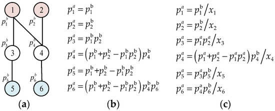
Figure 1.
Illustration of computing of node i. (a) Attack graph. (b) No MTD deployment. (c) Under MTD deployment.
In the scenario considered in this study, MTD can be applied to any node, but there is a limited budget for deploying MTD. The number of backup components of node i denotes the number of MTD candidates used at node i. Figure 1c illustrates how to calculate when MTD is deployed. Given this scenario, the problem of minimize the security loss (denoted by ) of the entire vulnerable system under the MTD strategy can be formulated as follows.
Equation (1) represents the objective function. Equation (2) means that the total cost of deploying backup components must not exceed the budget. In Equation (2), each is a non-negative integer. is calculated as in Equation (3).
In Figure 1c, init = {node1, node 2}.
3.2. Markov Decision Process
We model the above mathematical problems as Markov decision processes (MDPs), as follows:
- State space at time step includes V, denoting the value of all nodes, denoting the set of successful exploitation probability of all nodes being compromised, the set of deployment cost of all nodes, and the residual budget .
- Action space means that at time step , a backup component can be selected for MTD deployment. It is worth noting that the action will not be executed when the remaining budget is insufficient to support the deployment.
- State transition: After selecting a backup component for performing MTD, the penetration of the system as well as the remaining budget will change.
- Reward function: To minimize the possible security loss value of all nodes, we define the reward at time step as , and indicates the possible security loss value of all nodes at time step . If the agent chooses an action that violates constraints, i.e., exceeding the remaining budget, the agent will receive a large penalty.
4. RL-Based MTD-DO Approach
This section presents DQN- and PPO-based algorithms, which can tackle the problem introduced in Section 3.
4.1. DQN-Based Algorithm
The essence of solving the MDP in Section 3.2 is to find a policy of maximizing the future cumulative discounted rewards . A reward function is introduced to compute the future cumulative discounted reward at time step as in Equation (4).
where is the maximum number of steps, and is a discount factor used to control the degree of emphasis on future rewards, with its values ranging from [0, 1]. A larger indicates a greater emphasis on future rewards.
The action-value function is employed to represent the cumulative discounted rewards obtained by taking action at state . It can be expressed as in Equation (5).
Different from traditional reinforcement learning algorithms, such as Q-learning, DQN pioneered the integration of deep learning and reinforcement learning. It utilizes a Deep Neural Network (DNN) instead of the traditional Q-table to record the Q-values for all state–action pairs, so it can handle the dimensional explosion problem caused by the complex state and action spaces. To this end, we propose a DQN-based algorithm to find the optimal deployment policy for the problem considered in this study. The process for updating Q-values in the DQN-based algorithm is as defined as in Equation (6).
where is the parameters of the DNN. To address the issue of instability during the training process of the DNN, the algorithm introduces two DNNs, a target network and an online network , into the training procedure. A loss function is employed for updating network parameters, as shown in (7).
Algorithm 1 summarizes the details of the proposed DQN-based algorithm. Firstly, the algorithm initializes an experience replay pool, which aims to improve the stability of the algorithm training by reducing the correlation between samples.
To strike a balance between exploration and exploitation, we adopt a linearly decaying strategy to ensure more exploration in the early stages of training and shifts towards more exploitation in later stages. During training, the agent selects an action depending on the state of the current environment at each step (lines 3–4). Then, the agent records the transition in the experience replay pool (line 6). Finally, the agent calculates the target Q-value and updates parameters by using stochastic gradient descent (lines 8–9).
| Algorithm 1 DQN-Based Algorithm | |
| Input: Node information , , , and total budget | |
| Output: The optimal backup deployment policy | |
| Initialize the experience pool Initialize the parameters of and , respectively | |
| 1: | For do: |
| 2: | For do: |
| 3: | Use probability to choose a random action |
| 4: | Otherwise choose |
| 5: | Execute , observe , next state and whether done |
| 6: | Add transition to |
| 7: | Sample random minibatch of transitions from |
| 8: | Set |
| 9: | Perform a gradient descent step with loss function |
| 10: | Update |
| 11: | End for |
| 12: | End for |
4.2. PPO-Based Algorithm
As a state-of-the-art deep reinforcement learning (DRL) algorithm, PPO tends to exhibit faster convergence and stronger training stability in highly dynamic environments compared to other DRL algorithms due to its better sampling complexity. To this end, we propose a PPO-based algorithm to determine the optimal deployment policy for the problem considered in this study.
In the context of the actor–critic framework, PPO consists of two DNNs: an actor network denoted as and a critic network denoted as , where and represent the corresponding parameters of these networks. Given an input state , the actor will output the probability distribution of actions , while the critic will output the value of the state . The function of can be expressed as in Equation (8).
The clipped surrogate objective function for updating can be formulated as in Equation (9).
where is the ratio between the old actor policy and new one. and are the clip factor and the coefficient, respectively. denotes an entropy bonus to encourage exploration. is the generalized advantage estimator (GAE), which is shown in Equation (10).
where is a tuning parameter of GAE.
The loss function for updating the parameters of the critic network can be defined as in (11)
Algorithm 2 describes the details of the PPO-based algorithm, involving two primary stages: an experience generation phase and a policy update phase. In the first phase, the agent selects an action based on the actor network corresponding to the current state. Subsequently, it receives the reward and the next state, estimates the advantages, and stores these parameters along with the current state in a memory buffer (lines 1–8). After experience collection, the algorithm starts the policy update phase, during which the actor network parameters and the critic network parameters will be updated epochs by optimizing the loss functions and , respectively (lines 9–11).
The process of completing the above two stages once is called one episode, and OPAR learns the optimal routing policy by iterating through episodes.
| Algorithm 2 PPO-Based Algorithm | |
| Input: Node information , , , and total budget | |
| Output: The optimal backup deployment policy | |
| 1: | For do: |
| 2: | Reset the environment |
| 3: | do: |
| 4: | and execute |
| 5: | and whether done |
| 6: | If done, reset the environment and continue |
| 7: | according to Equation (10) |
| 8: | End for |
| 9: | For k = 1, 2, , K do |
| 10: | Update and separately according to Equations (9) and (11) |
| 11: | End for |
| 12: | End for |
5. Experiment Evaluation
This section first gives a detailed description of the experiment parameters and our algorithm parameters in Section 5.1 and Section 5.2, respectively. Then, two baselines and experimental results are given in Section 5.3.
5.1. Experiment Setting
Figure 2 describes the attack graph for experiments, which is part of the attack graph of a realistic SCADA system developed in [26]. The yellow nodes represent nodes which can be accessed from outside, the green nodes represent middle nodes in an attack path, and red nodes represent critical nodes. The arrows denote the attack path from greed nodes to red nodes. Since the critical nodes are of an extreme value, we assume these nodes have a value of 100, markedly higher than other nodes, whose values range from 5 to 10. of each node is randomly generated, with a range of values between 0 and 1. The deployment cost for backup components at different nodes varies within the range of [30, 70]. With a fixed budget, a certain number of components are deployed at specific nodes to minimize the potential loss of the overall system.
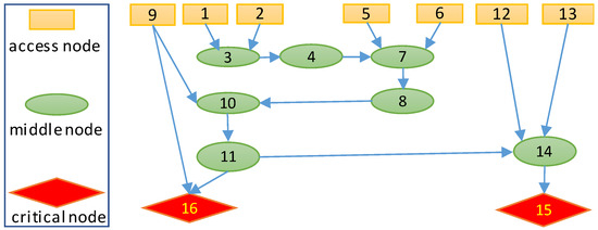
Figure 2.
An attack graph of 16-node scenario.
5.2. Training Details
All experiments in this study use PyTorch 1.5 as the code framework. The hardware configuration consists of an Intel(R) Xeon(R) Gold 6230 CPU @ 2.10 GHz, with 256 G RAM and two NVIDIA RTX 4090 GPUs. The operation system is Ubuntu 20.04. Table 2 gives the experiment settings.
Table 2.
Scenario setting.
To find the optimal hyper-parameters for the algorithms, we first train the DQN-based algorithm using different learning rates and batch sizes in the 16-node scenario, and the results are illustrated in Figure 3. It can be observed that increasing the learning rate and batch size accelerates the convergence speed of the algorithm. Simultaneously, the algorithm converges successfully under the majority of hyper-parameter combinations. However, when the learning rate and batch size are large, such as a learning rate of 0.005 and a batch size of 64, the algorithm exhibits some oscillations. To ensure the best training results, we set the learning rate to 0.005 and the batch size to 64 in the subsequent experiments. A similar method is used to obtain the optimal hyper-parameters of the PPO-based algorithm. Table 3 gives the algorithm settings.
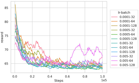
Figure 3.
Training results of DQN algorithm under different hyper-parameters.
Table 3.
Summary of algorithm setting.
5.3. Performance Comparison
Our literature investigation indicates that there is no existing work considering our MTD-DO problem. Moreover, it is hard, if not impossible, to extend the existing algorithms to address the MTD-DO problem. Thus, we compare our algorithms with the following two baselines for evaluation:
- (1)
- Q-learning algorithm. Q-learning is a classic model-free reinforcement learning algorithm that generates an optimal policy by maintaining a Q-table composed of state–action pairs.
- (2)
- Random algorithm. It is a simple heuristic algorithm that randomly selects a node for deployment, excluding under-budgeted nodes.
We train both the proposed algorithms and the two baseline algorithms in the experiment scenarios and compare their respective training effects. Simultaneously, for each scenario, we set total budgets to examine the influence of budget on algorithm training. To mitigate the impact of randomness, all algorithms were trained five times with different random seeds.
To enable a comparative assessment of backup deployment strategies generated by the four algorithms, we introduce a loss-avoidance metric . This metric indicates the extent to which the backup deployment strategy mitigates the potential value loss , and it is defined in Equation (12).
where is the overall potential loss value after deployment and is the initial potential loss value.
Figure 4 shows the experimental results. It can be observed that, under a fixed budget, as the number of nodes increases, the final values of obtained by all algorithms gradually increase. The reason is that the same budget implies the number of deployable backup components remains approximately unchanged. As the number of nodes increases, the impact of these backup components will be weakened. Therefore, to ensure the effective enhancement of the overall security of the system, it is advisable to appropriately increase the budget when the number of nodes increases.
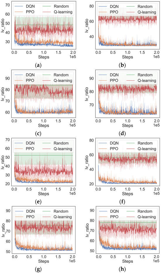
Figure 4.
Training results of DQN, PPO, Q-learning, and random algorithms, respectively, in multiple scenario settings. (a) , (b) , (c) , (d) , (e) , (f) , (g) , (h) .
Then, we analyze the performance of the algorithms. As is shown in Figure 4, the performance of the Q-learning algorithm is noticeably superior to the random algorithm in smaller-scale scenarios like C = 200 and n = 8. However, as the scenario scale increases, Q-learning begins to fail and performs similarly to the random algorithm. This phenomenon can be attributed to the expansion of the state and action spaces associated with the increase in scenario scale, posing a challenge for Q-learning to cope with the issue of dimensionality explosion.
As can be seen in Figure 4, in contrast to Q-learning, both the DQN-based algorithm and the PPO-based algorithm utilize DNNs to approximate value functions, resulting in superior performance across all experiment scenarios. The DQN-based algorithm has the fastest convergence speed compared to the PPO-based algorithm in all scenario settings. Additionally, in the scenarios where the total budget is equal to 300, the DQN-based approach produces results that are marginally ahead of those with the PPO-based approach. One possible reason is that the problem addressed in this study involves highly discrete state and action spaces and is well suited to be solved by the DQN-based algorithm.
In addition, in the 16-node scenario, we explore the cases where the total budget is 100, 400, and 500. The algorithm training results are shown in Figure 5a. It can be noticed that with an increase in budget, the steadily decreases. The reason is that a higher budget implies the ability to deploy additional backup components, thereby reducing the probability of successful exploitation of the nodes in the system. However, increasing the total budget exhibits a noticeable diminishing marginal return effect, meaning that as the total budget continues to increase, the incremental benefits derived from it gradually decrease. For clarity, we introduce a metric to represent the benefits derived from the unit budget, which can be expressed as in Equation (13).
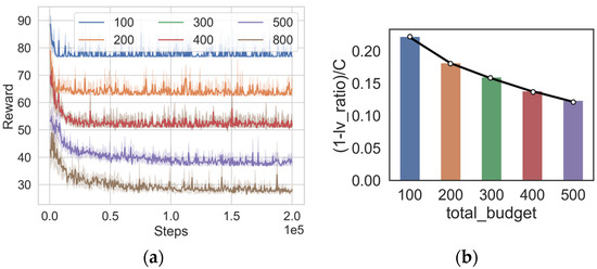
Figure 5.
Training results of DQN algorithm under different budgets (a) , (b) .
The values of metrics corresponding to different budgets are shown in Figure 5b. It can be observed that with an increase in cost, the cost-effectiveness of the unit cost is gradually decreasing. Given that costs are often a crucial factor in reality, it becomes essential to achieve a balance between costs and benefits. Our algorithms can assist in determining the optimal budget by generating deployment strategies under different budgets, demonstrating its practical application value.
5.4. Discussion
This subsection summarizes some conclusions from the experiments.
- (1)
- (2)
- The budget should be appropriately increased when the number of nodes increases. As the number of nodes in the attack graph increases, the impact of these backup components will be weakened. See Figure 4. When the number of nodes varies from 8 to 9, there is large security increase, but from 15 to 16, the increase is small.
- (3)
- DRL-based algorithms work well over various scenarios. Scalability is an important metric for evaluating an algorithm. In the scenario investigated in this study, both the attack graph size and the budget affect the problem size. The larger the budget, the more backup components. Figure 4 is about the attack graph size, and Figure 5 is about the budget amount. These results are illustrated in Figure 4g,h.
6. Conclusions and Future Work
In this study, we propose two DRL-based algorithms in optimizing MTD deployment effectiveness in terms of minimizing the security threat in an attack graph within the limited budget. The design of DQN-based and PPO-based algorithms is detailed. The experiment results indicate that both the PPO- and DQN-based algorithms perform better than Q-learning-based and random algorithms. The DQN-based algorithm converges best. In terms of reward, the DQN-based algorithm performs marginally better than the PPO-based algorithm.
This study only considers security and the cost of deploying MTD. It is known that MTD deployment will bring about a service performance degradation. How to balance the tradeoff of security, cost, and service performance will be considered in our future works. Additionally, this study assumes that the knowledge of the system threats is available. It is interesting to combine the risk prediction mechanisms with our approach and then make dynamic deployment decisions. Finally, in this study, we did not consider the operations of MTD technologies at each component. Investigating the impact of these operations will be one future research direction, and we will design more efficient DRL-based algorithms for time-sensitive scenarios.
Author Contributions
Conceptualization, Q.L.; investigation and methodology, Q.L.; writing—original draft preparation, Q.L.; writing—review and editing, Q.L. and J.W.; software, Q.L.; validation, Q.L. All authors have read and agreed to the published version of the manuscript.
Funding
This research received no external funding.
Institutional Review Board Statement
Not applicable.
Data Availability Statement
Data are contained within the article.
Conflicts of Interest
The authors declare no conflicts of interest.
References
- Pagnotta, G.; De Gaspari, F.; Hitaj, D.; Andreolini, M.; Colajanni, M.; Mancini, L.V. DOLOS: A Novel Architecture for Moving Target Defense. IEEE Trans. Inf. Forensics Secur. 2023, 18, 5890–5905. [Google Scholar] [CrossRef]
- Rehman, Z.; Gondal, I.; Ge, M.; Dong, H.; Gregory, M.A.; Tari, Z. Proactive defense mechanism: Enhancing IoT security through diversity-based moving target defense and cyber deception. Comput. Secur. 2024, 139, 103685. [Google Scholar] [CrossRef]
- Tech, G.E. Security—Tech Innovators in Automated Moving Target Defense; Pohto, M., Manion, C., Eds.; Gartner: Singapore, 2023. [Google Scholar]
- Ma, H.; Han, S.; Kamhoua, C.A.; Fu, J. Optimizing Sensor Allocation Against Attackers with Uncertain Intentions: A Worst-Case Regret Minimization Approach. IEEE Control Syst. Lett. 2023, 7, 2863–2868. [Google Scholar] [CrossRef]
- Yoon, S.; Cho, J.-H.; Kim, D.S.; Moore, T.J.; Free-Nelson, F.; Lim, H. Attack Graph-Based Moving Target Defense in Software-Defined Networks. IEEE Trans. Netw. Serv. Manag. 2020, 17, 1653–1668. [Google Scholar] [CrossRef]
- Javadpour, A.; Ja, F.; Taleb, T.; Shojafar, M.; Yang, B. SCEMA: An SDN-Oriented Cost-Effective Edge-Based MTD Approach. IEEE Trans. Inf. Forensics Secur. 2023, 18, 667–682. [Google Scholar] [CrossRef]
- Sun, F.; Zhang, Z.; Chang, X.; Zhu, K. Toward Heterogeneous Environment: Lyapunov-Orientated ImpHetero Reinforcement Learning for Task Offloading. IEEE Trans. Netw. Serv. Manag. 2023, 20, 1572–1586. [Google Scholar] [CrossRef]
- Zhang, T.; Xu, C.; Lian, Y.; Tian, H.; Kang, J.; Kuang, X.; Niyato, D. When Moving Target Defense Meets Attack Prediction in Digital Twins: A Convolutional and Hierarchical Reinforcement Learning Approach. IEEE J. Sel. Areas Commun. 2023, 41, 3293–3305. [Google Scholar] [CrossRef]
- MRibeiro, A.; Fonseca, M.S.P.; de Santi, J. Detecting and mitigating DDoS attacks with moving target defense approach based on automated flow classification in SDN networks. Comput. Secur. 2023, 134, 103462. [Google Scholar] [CrossRef]
- Celdrán, A.H.; Sánchez, P.M.S.; von der Assen, J.; Schenk, T.; Bovet, G.; Pérez, G.M.; Stiller, B. RL and Fingerprinting to Select Moving Target Defense Mechanisms for Zero-Day Attacks in IoT. IEEE Trans. Inf. Forensics Secur. 2024, 19, 5520–5529. [Google Scholar] [CrossRef]
- Zhou, Y.; Cheng, G.; Ouyang, Z.; Chen, Z. Resource-Efficient Low-Rate DDoS Mitigation with Moving Target Defense in Edge Clouds. IEEE Trans. Inf. Forensics Secur. 2024, 19, 6377–6392. [Google Scholar] [CrossRef]
- Li, L.; Ma, H.; Han, S.; Fu, J. Synthesis of Proactive Sensor Placement in Probabilistic Attack Graphs. In Proceedings of the 2023 American Control Conference (ACC), San Diego, CA, USA, 31 May–2 June 2023; pp. 3415–3421. [Google Scholar]
- Ghourab, E.M.; Naser, S.; Muhaidat, S.; Bariah, L.; Al-Qutayri, M.; Damiani, E.; Sofotasios, P.C. Moving Target Defense Approach for Secure Relay Selection in Vehicular Networks. Veh. Commun. 2024, 47, 100774. [Google Scholar] [CrossRef]
- Mnih, V. Human-level control through deep reinforcement learning. Nature 2015, 518, 529–533. [Google Scholar] [CrossRef] [PubMed]
- Schulman, J.; Wolski, F.; Dhariwal, P.; Radford, A.; Klimov, O. Proximal policy optimization algorithms. arXiv 2017, arXiv:1707.06347. [Google Scholar]
- Kang, H.; Chang, X.; Misic, J.V.; Misic, V.B.; Fan, J.; Liu, Y. Cooperative UAV Resource Allocation and Task Offloading in Hierarchical Aerial Computing Systems: A MAPPO-Based Approach. IEEE Internet Things J. 2023, 10, 10497–10509. [Google Scholar] [CrossRef]
- Zenitani, K. Attack graph analysis: An explanatory guide. Comput. Secur. 2023, 126, 103081. [Google Scholar] [CrossRef]
- Cho, J.-H.; Sharma, D.P.; Alavizadeh, H.; Yoon, S.; Ben-Asher, N.; Moore, T.J.; Kim, D.S.; Lim, H.; Nelson, F.F. Toward proactive, adaptive defense: A survey on moving target defense. IEEE Commun. Surveys Tuts. 2020, 22, 709–745. [Google Scholar] [CrossRef]
- Chang, X.; Shi, Y.; Zhang, Z.; Xu, Z.; Trivedi, K.S. Job Completion Time Under Migration-Based Dynamic Platform Technique. IEEE Trans. Serv. Comput. 2022, 15, 1345–1357. [Google Scholar] [CrossRef]
- Chen, Z.; Chang, X.; Han, Z.; Yang, Y. Numerical Evaluation of Job Finish Time Under MTD Environment. IEEE Access 2020, 8, 11437–11446. [Google Scholar] [CrossRef]
- Santos, L.; Brito, C.; Fé, I.; Carvalho, J.; Torquato, M.; Choi, E.; Lee, J.-W.; Nguyen, T.A.; Silva, F.A. Event-Based Moving Target Defense in Cloud Computing with VM Migration: A Performance Modeling Approach. IEEE Access 2024. [Google Scholar] [CrossRef]
- Nguyen, M.; Samanta, P.; Debroy, S. Analyzing Moving Target Defense for Resilient Campus Private Cloud. In Proceedings of the 2018 IEEE 11th International Conference on Cloud Computing (CLOUD), San Francisco, CA, USA, 2–7 July 2018; pp. 114–121. [Google Scholar]
- Tan, J.; Jin, H.; Hu, H.; Hu, R.; Zhang, H.; Zhang, H. WF-MTD: Evolutionary Decision Method for Moving Target Defense Based on Wright-Fisher Process. IEEE Trans. Dependable Secur. Comput. 2023, 20, 4719–4732. [Google Scholar] [CrossRef]
- Umsonst, D.; Saritas, S.; Dán, G.; Sandberg, H. A Bayesian Nash Equilibrium-Based Moving Target Defense Against Stealthy Sensor Attacks. IEEE Trans. Autom. Control 2024, 69, 1659–1674. [Google Scholar] [CrossRef]
- Singhal, A.; Ou, X. Security Risk Analysis of Enterprise Networks Using Probabilistic Attack Graphs. In Network Security Metrics; Springer: Gaithersburg, MD, USA, 2017. [Google Scholar]
- Haque, M.A.; Shetty, S.; Kamhoua, C.A.; Gold, K. Integrating Mission-Centric Impact Assessment to Operational Resiliency in Cyber-Physical Systems. In Proceedings of the GLOBECOM 2020—2020 IEEE Global Communications Conference, Taipei, Taiwan, 7–11 December 2020; pp. 1–7. [Google Scholar]
Disclaimer/Publisher’s Note: The statements, opinions and data contained in all publications are solely those of the individual author(s) and contributor(s) and not of MDPI and/or the editor(s). MDPI and/or the editor(s) disclaim responsibility for any injury to people or property resulting from any ideas, methods, instructions or products referred to in the content. |
© 2024 by the authors. Licensee MDPI, Basel, Switzerland. This article is an open access article distributed under the terms and conditions of the Creative Commons Attribution (CC BY) license (https://creativecommons.org/licenses/by/4.0/).