Abstract
Solving the Perspective-n-Point (PnP) problem is difficult in low-power systems due to the high computing workload. To handle this challenge, we present an originally designed FPGA implementation of a PnP solver based on Vivado HLS. A matrix operation library and a matrix decomposition library based on QR decomposition have been developed, upon which the EPnP algorithm has been implemented. To enhance the operational speed of the system, we employed pipeline optimization techniques and adjusted the computational process to shorten the calculation time. The experimental results show that when the number of input data points is 300, the proposed system achieves a processing speed of 45.2 fps with a power consumption of 1.7 W and reaches a peak-signal-to-noise ratio of over 70 dB. Our system consumes only 3.9% of the power consumption per calculation compared to desktop-level processors. The proposed system significantly reduces the power consumption required for the PnP solution and is suitable for application in low-power systems.
1. Introduction
The Perspective-n-Point (PnP) problem is the problem of determining the pose of a calibrated camera from n correspondences between 3D reference points and their 2D projections [1]. It is widely used in visual SLAM [2,3], robotics [4], and Augmented Reality [5]. Typically, the PnP algorithm is implemented by the CPU. However, in embedded systems, the processing speed of the processor is relatively slow, and the high computational complexity of the PnP algorithm leads to the inability of real-time calculations. Although PC processors bring considerable computational speed, their high-power consumption makes it difficult to apply them in low-power systems, such as battery-powered robots and VR glasses.
To reduce power consumption and latency, hardware acceleration is often considered a feasible method of algorithmic acceleration. It provides faster computing speed while using little power. Despite the potential benefits of hardware acceleration, currently, there is no published hardware implementation of the PnP algorithm. The lack of a hardware implementation is primarily attributed to algorithm complexity.
The difficulties of hardware design for PnP solvers mainly stem from the following three aspects. Firstly, during the calculation process, the data exhibit strong dependencies, and some data are used multiple times, making pipelining difficult to achieve and increasing the difficulty of data management.
Secondly, the diversity of input data leads to a wide dynamic range of numbers during the calculation process, posing a significant challenge in maintaining reasonable hardware costs while ensuring calculation accuracy by using fixed-point numbers. It is also difficult to use floating-point numbers in hardware design due to poor support offered by hardware description language.
Thirdly, during the computation process, various math functions are required, such as the computation of square roots and the solution for matrix eigenvalues, which cannot be simply computed by calling libraries as easily as in software. For this reason, most current PnP-solving processes are based on processors.
In this paper, we propose an FPGA accelerator for solving the PnP problem, which enables real-time computational performance with high energy efficiency. To overcome the challenges of implementing the PnP solving algorithm on hardware, we utilize high-level synthesis (HLS) languages to ease the developing process. HLS languages are capable of translating high-level languages such as C/C++ into register transfer level (RTL) languages [6,7], allowing hardware implementation to be directly realized with high-level languages, which simplifies the process of hardware implementation design. The results obtained show that the proposed system achieves real-time processing speed, while its energy consumption is significantly lower than that of systems based on processors.
The contributions of this paper can be summarized as follows.
- (1)
- Solving the PnP problem is useful in many applications, but so far there is no hardware solver due to complexity. To the best of our knowledge, the proposed accelerator in this paper makes the first attempt to implement a hardware PnP solver on FPGA.
- (2)
- To achieve a complete PnP solution, we developed a functional module for solving matrix eigenvalues, eigenvectors, and linear least squares equations using QR decomposition. The module can be used as a reference for other designs.
- (3)
- We carefully fine-tuned the system to achieve maximum performance. To compare the performance of the proposed system with others, experiments were carried out on different platforms. The results indicate that the proposed system exhibits superior performance in terms of energy efficiency.
The rest of the paper is organized as follows: Section 2 introduces related work on solving the PnP problem. Section 3 describes the hardware architecture of the proposed system. Section 4 describes the obtained optimization methods. Section 5 shows the experimental results of the system. Section 6 summarizes the paper.
2. Related Work
Efforts have been made to optimize the speed and accuracy of solving the PnP problem. Most of them focus on the improvement of software algorithms.
The core of solving the PnP problem is to determine the camera pose based on 3D reference points and their 2D projected points. The minimum number of points required to solve this problem is three. In this case, the PnP problem is transformed into a P3P [8] problem. Accordingly, when the number of points is 4 or 5, the PnP problem transforms into P4P and P5P problems, respectively. Although solving the PnP problem with a small number of points is possible, the results can become inaccurate under noise [9]. By using more points, the accuracy of the calculation can be significantly improved.
Most PnP solution algorithms support input of an arbitrary number of points and can be broadly classified into two categories: iterative and non-iterative methods [10]. Iterative methods approach the PnP problem as an optimization problem between 3D reference points and 2D projected points. They represent the error through a nonlinear cost function [11,12] and then employ iterative optimization techniques, such as the Gauss–Newton method and the Levenberg–Marquardt method, to minimize this error. When the algorithm converges correctly, iterative algorithms tend to achieve higher accuracy, but their computational process is more complex, resulting in a heavier computational burden. Iterative methods may fall into local minima, leading to incorrect calculation results [11].
Non-iterative algorithms avoid the multiple calculations and adjustments that may be required during the iterative process. These algorithms have a lower dependence on initial values because they do not rely on the gradual approximation in the iterative process. The Direct Linear Transformation (DLT) [13] is a viable method for solving the PnP problem. However, it ignores some important inherent constraints, such as the orthogonality and unitarity of the rotation matrix, which may affect the stability and accuracy of the results. To improve accuracy, various methods have been proposed, but some of these algorithms have a relatively high computational complexity. For example, [14] with , [15] with , or even [16] with . EPnP [1] is an efficient non-iterative algorithm with linear complexity, it utilizes four sets of virtual “control points” to represent all actual points, and by solving for the positions of these control points in the camera coordinate system, it realizes high-precision pose estimation.
Although previous work has improved the speed and accuracy of solving the PnP problem algorithmically, they have not explored implementation methods other than using CPUs. Furthermore, these algorithmic improvements rarely take into account the power consumption during the computational process of the algorithms. In this work, we improve the PnP solver from the hardware level, focusing on reducing power consumption during the algorithm execution process, while ensuring accuracy and speed.
In the proposed system, we utilize the EPnP algorithm proposed in [1]. The choice of the EPnP algorithm is primarily based on the following considerations: Firstly, the EPnP algorithm is a non-iterative method with linear complexity, which implies that its efficiency advantage is evident regardless of whether the data comprises four points or hundreds of points. The EPnP algorithm is significantly faster than iterative algorithms and algorithms with high complexity, which is crucial for real-time PnP computation. Furthermore, the EPnP algorithm not only ensures computational efficiency but also achieves high positioning accuracy. The EPnP algorithm can further enhance the pose estimation accuracy through post-optimization. Therefore, by using the EPnP algorithm to construct a hardware accelerator, there will be minimal loss of precision during the computation process. In addition, the EPnP algorithm allows for parallel computation, such as in the process of matrix multiplication, which can fully utilize the parallel computing capabilities of FPGAs, thereby accelerating the calculation speed.
3. Hardware Architecture
3.1. Overview of the System
A high-level block diagram of the proposed system is shown in Figure 1. The proposed PnP solving accelerator consists of three main components: matrix calculation, QR decomposition (QRD), and PnP solution.
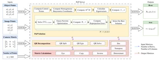
Figure 1.
High-level block diagram of the proposed PnP solving accelerator.
The input data of the proposed system are 3D reference points and their 2D projections, the camera matrix, as well as the number of point pairs used in the calculation process. The output data are the camera pose. The number of input point pairs for PnP calculation varies with different applications. Depending on the number of input point pairs, the amount of storage space required during the calculation process also varies. Given the limitation of FPGA devices in facilitating dynamic memory allocation, it is necessary to allocate memory space in advance. After weighing the trade-off between the practicality of the design and the consumption of hardware resources, the proposed system has been designed to support the calculation of a maximum of 512 points.
During the solution process of the PnP algorithm, there are significant differences in the dynamic range of data based on different input data. When using fixed-point numbers to store and compute data, in order to avoid both overflow and loss of precision, a higher bit width is required. To reduce the trouble of fixed-point conversion during the computation process, all decimal data are stored and computed as 32-bit floating-point numbers. Thanks to the HLS tool, the computation of floating-point arithmetic becomes straightforward, which is challenging to accomplish with RTL code.
Except for the number of point pairs, the input and output interfaces of the solver core are implemented as block RAM interfaces. In each clock cycle, a floating-point number can be retrieved from or stored in the block RAM. Additionally, users are allowed to specify the number of points involved in the calculation by changing the parameter n, which is implemented as a vector. During the computation process, the first n points of data stored in the block RAM are utilized, while the subsequent data are ignored, thus enabling the adjustment of the number of point pairs involved in the computation.
In addition to the input and output data signals, the solver core also carries control signals that initiate the computation process and indicate the completion of the computation. To use the solver core, users need to implement the external logic for initializing the solver core on the FPGA. The coordinates of the reference point, the projection point, and the camera matrix are first written into the block RAM. Then, the number of points to be used in the calculation is specified, and finally, the solver core is initiated to start the computation. After the computation is completed, the camera pose can be read from the block RAM. The solver core independently completes the PnP calculation without the involvement of other modules, achieving hardware acceleration for solving the PnP problem. During this process, the solver core is not responsible for data interaction with external circuits, and additional logic circuits need to be implemented to realize data transmission.
3.2. Basic Matrix Calculations
In the process of solving the PnP problem, certain matrix operations are required. Performing matrix operations on hardware is not as simple as on a processor. Despite the powerful capabilities of HLS tools, designing efficient hardware still requires extensive experience and design skills. This is mainly due to the limitation of FPGA storage methods, which cannot dynamically allocate memory during the computation process, making it impossible to directly use existing C++ libraries like Eigen [17] in HLS designs. Works such as [18] have attempted to design matrix operation libraries based on HLS, but due to their non-opensource nature, we have developed a library containing a set of basic matrix operations that can be synthesized in the HLS environment on our own. The functionalities of the library are shown in Table 1. By encapsulating matrix operations into modular functions, we facilitate a unified approach to configuring parallel optimization strategies for matrix computations within the HLS tools, while also enhancing the reusability of the code.

Table 1.
Supported matrix operations.
In order to reduce the complexity of implementation, thereby reducing the hardware resources occupied by the FPGA implementation and optimizing the computation speed, this matrix library only implements the necessary matrix operations and dimensions in the EPnP solution. Since the determinant is only required when calculating the rotation matrix R, while R is a matrix, the determinant function is only implemented for matrices. For other matrix operations, arbitrary dimensions within a certain range are supported. Due to the limitation that FPGAs cannot dynamically allocate memory, these functions pre-allocate storage space based on the maximum matrix dimension during the computation process. In this way, there is enough space to save temporary data during the calculation process.
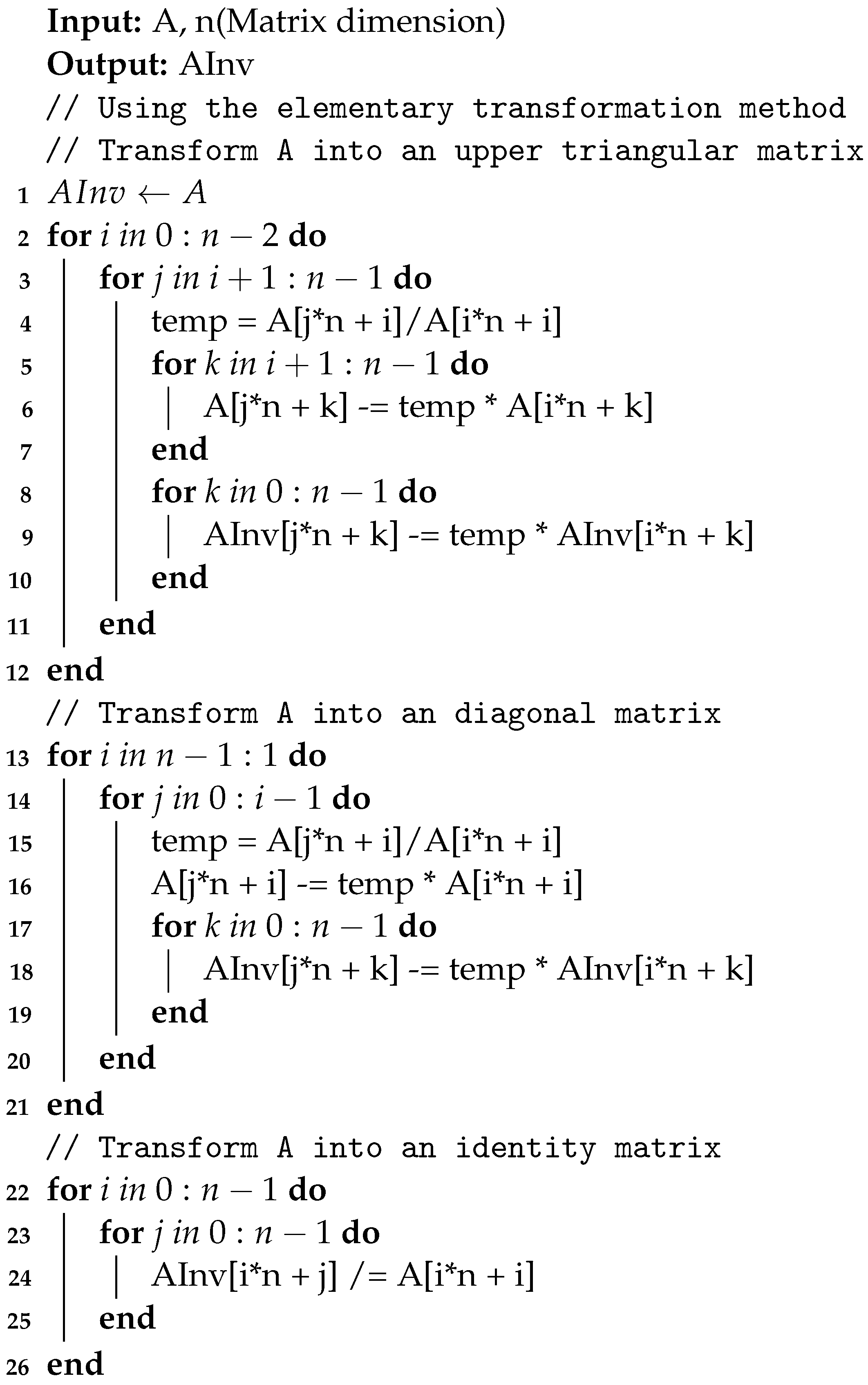
The parameters of the functions include pointers to input and output arrays, as well as the dimensions of the matrices. The HLS tool synthesizes the matrices into block RAMs, where it reads data from the input block RAMs based on the matrix size during the computation process, performs the calculations, and then writes the results back to the output block RAMs. The implementation is identical to C++ in other respects. For example, the matrix inversion operation can be expressed in Algorithm 1.
| Algorithm 1: Matrix Inversion. |
 |
Compared to implementing Verilog, HLS places more emphasis on the computational process of data, eliminating the trouble of manually controlling the flow through state machines. Users can focus their attention on the implementation of the algorithm.
3.3. QR Decomposition Module
QR decomposition is used to solve matrix eigenvalues, eigenvectors, and solutions to homogeneous linear equations. QR decomposition breaks down a matrix into an orthogonal matrix Q and an upper triangular matrix R. Through iterative methods, the original matrix can be gradually transformed into an approximately upper triangular matrix, thereby facilitating the solution of eigenvalues. This decomposition method is computationally more efficient, especially for large matrices, as it significantly reduces the amount of computation. Additionally, due to the properties of orthogonal matrices, QR decomposition exhibits high numerical stability, contributing to more accurate eigenvalue solutions. The QR decomposition method for solving eigenvalues can be applied to various types of matrices, including real symmetric matrices and complex matrices. In the process of solving eigenvalues and eigenvectors, the QR algorithm typically demonstrates fast convergence rates. This implies that, with the same number of iterations, the QR algorithm can approximate the true eigenvalues and eigenvectors more quickly, thereby enhancing the efficiency of the solution. Apart from QR decomposition, there exist other methods for solving eigenvalues and eigenvectors, but they come with their own limitations. For instance, the inverse matrix method requires the matrix to be invertible, the Jacobi iteration method necessitates the matrix to be symmetric, and the method based on the definition involves solving a high-degree polynomial equation. In terms of practical applicability and convergence speed, these methods often pale in comparison to the QR decomposition approach.
The hardware architecture of the QRD module consists of three parts: QR split, QR egis, and QR solve. A functional block diagram of the QRD module is shown in Figure 2.
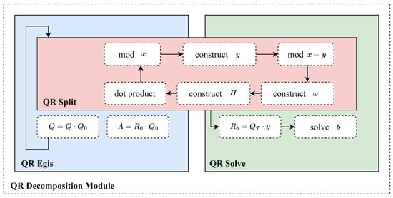
Figure 2.
Hardware architecture of the QR decomposition module.
The QR egis module and the QR solution module share the same QR split module. When a matrix is decomposed, the result can be utilized to compute eigenvalues and eigenvectors by the QR Egis module, or for solving linear least squares problems by the QR Solve module.
3.3.1. QR Split
QR split module factors an matrix A into the product of an orthogonal matrix Q and an upper triangular matrix R. QR split can be implemented through various algorithms, including the Gram–Schmidt algorithm [19], the Householder algorithm [20], the Givens algorithm [21,22], the Modified Gram-Schmidt algorithm [23,24] and so on. Among them, the Householder algorithm is widely used due to its numerical stability. In the proposed system, a QR split based on Householder transformation is implemented, which can be expressed in Algorithm 2.
| Algorithm 2: Householder QR. |
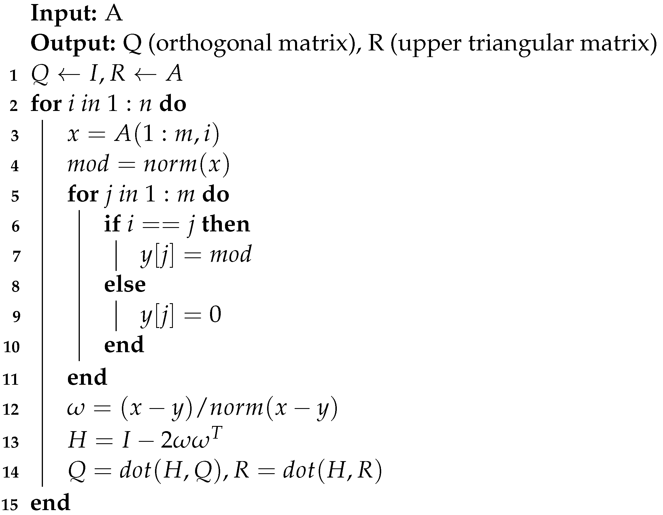 |
In Algorithm 2, A is the input matrix, and Q and R are the output matrices. After initializing matrix Q as the identity matrix and matrix R as the input matrix, the modulus of the first column vectors of A is first calculated, which is used to construct the unit vector . Next, a Householder matrix H is constructed and multiplied by matrices Q and R. At this point, all elements in the first column of matrix R, except the first element, are reduced to 0. The same operation is performed on the remaining columns of the input matrix in sequence, since the Householder matrix H is orthogonal, its cumulative product result Q is also an orthogonal matrix, and R is reduced to an upper triangular matrix.
For FPGA implementation, the norm function is replaced by first computing the sum of squares of the vector elements and then taking the square root of that sum. The square root can be calculated using the sqrt function provided by HLS tools, eliminating the need to use the CORDIC core. Note that in Algorithm 2, there are two loops. The sub-loop is used to initialize the vector y, and since the computations within the loop are independent of each other, they can be unrolled to take advantage of parallel computing on an FPGA. However, in the parent loop, the Q and R matrices are generated iteratively, so the loop cannot be unrolled. It must wait for one iteration to complete before starting the next iteration.
3.3.2. QR Egis
The QR Egis module implements an iterative method for computing eigenvalues and eigenvectors, using Algorithm 3.
| Algorithm 3: QR Egis. |
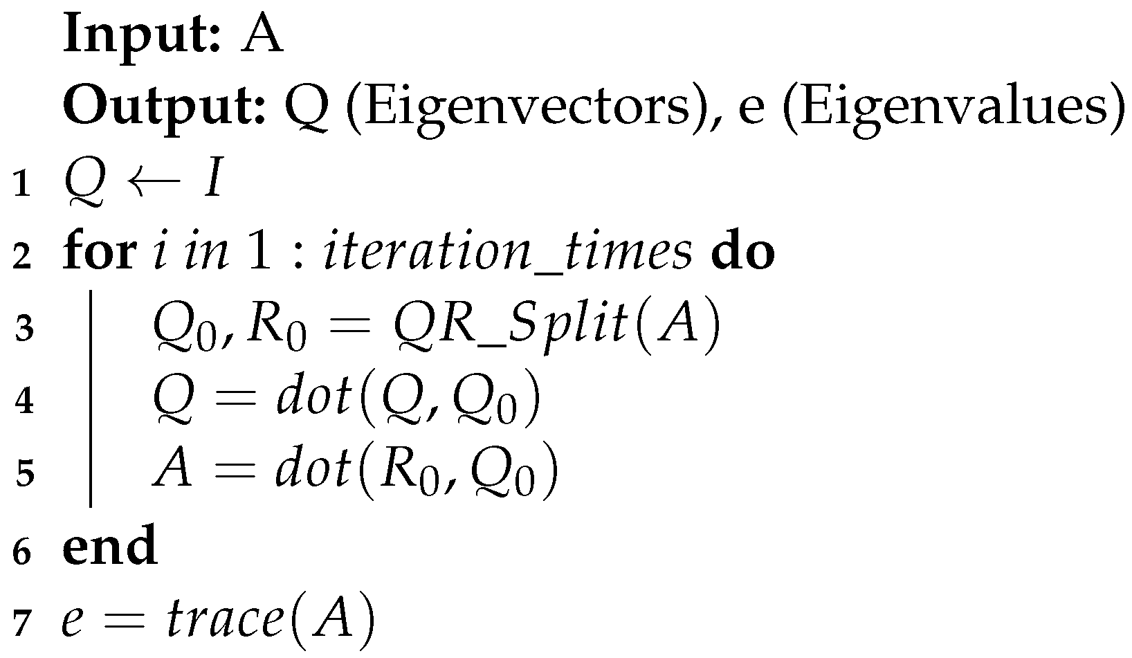 |
At the beginning, matrix Q is initialized as the identity matrix. By repeatedly performing QR decomposition on matrix A and multiplying the obtained orthogonal matrices together, the matrix Q gradually approaches the eigenvector matrix. When matrix A converges approximately to an upper triangular matrix, the iteration is complete, and the main diagonal elements are then the eigenvalues.
The number of iteration times determines the accuracy and speed of the calculation. As the number of iterations increases, the result becomes more precise, but the computation time also increases. Figure 3 demonstrates the influence of the number of iterations on the accuracy and computational time of QRD. The peak signal-to-noise ratio () is defined as
where is the value of the largest element in the result matrix, and stands for Mean Squared Error, which is the minimum squared error between the output matrix and the true value.
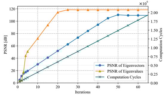
Figure 3.
The relationship between iterations and PSNR as well as computational speed.
As the number of iterations increases, the computational time grows linearly, while the errors of eigenvalues and eigenvectors continue to decrease and finally stabilize. When the number of iterations is small, the results exhibit significant errors due to non-convergence. However, once the number of iterations increases to a certain value, the errors are primarily influenced by floating-point precision, rendering further increases in iteration count ineffective in improving the results. Since the computation time for each iteration is the same, the number of computation cycles grows linearly with the number of iterations.
The proposed system selects the number of iterations as 10 because the data accuracy can already fulfill the precision demands of the PnP problem at this point. Selecting an excessively large number of iterations can lead to a protracted computation time.
3.3.3. QR Solve
The QR solution module is used for solving linear least squares problems. Its core objective is to find a set of solutions that minimize the sum of squared errors between the model’s predicted values and the actual observed values when an exact solution to a set of linear equations does not exist. The form of the system of equations is given as
When the matrix A can be factored into the product of an orthogonal matrix Q and an upper triangular matrix R through QR decomposition, the equation transforms into
i.e.,
Since R is an upper triangular matrix, the solution to the equation can be obtained using Algorithm 4:
| Algorithm 4: QR Spilt. |
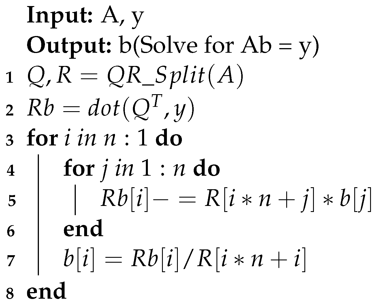 |
3.4. PnP Solution
The PnP solution is the core function of the system. During the PnP solution process, the same set of data is used multiple times during the computation, which poses difficulties in synchronizing the functional modules. In this design, when a portion of the hardware circuitry is performing a computation, the remaining circuitry remains in an inactive mode, and only after the computation is completed will the subsequent computation be initiated, thereby ensuring the correctness of the results. Since there were no major modifications made to the EPnP algorithm, the computational process of the PnP solver remains the same as that of the original algorithm. First, four control points are determined based on the world coordinates. For each world coordinate, homogeneous barycentric coordinates are calculated based on the control points. Next, matrix M is constructed with each reference point, and the product is calculated simultaneously. Upon the completion of computation, the eigenvectors of this matrix are calculated. Then, the matrix L is formed with eigenvectors, and is derived from control points.
We compute solutions for all four distinct values of N, which is the effective dimension of the null space, and subsequently select the optimal solution that minimizes the reprojection error, thereby ensuring the highest level of accuracy and precision. During the computation process, some data will be used multiple times, and these data are stored in BRAM. When these data are being read and written, they cannot be accessed simultaneously by other modules, so the entire PnP solution process is executed sequentially in the order of the algorithm.
4. Optimization
4.1. Pipelining
Pipelining is a frequently employed optimization strategy in FPGA design that enables concurrent hardware execution, thereby significantly elevating computational performance. In the traditional RTL design method, designers need to manually control the data flow, dividing the computing process into multiple steps and allocating them to several clock cycles. In HLS implementation, designers only need to set the pipeline parameters, and the HLS tool will automatically implement the pipeline.
In the process of solving the PnP problem, matrix multiplication is a time-consuming process. The core of matrix multiplication is multiplication–accumulation, which consists of four stages: data loading, floating-point multiplication, floating-point addition, and data saving. A single multiplication-accumulation process requires eight clock cycles, as shown in Figure 4. Before pipelining is implemented, the next operation can only be executed after the previous one is completed, resulting in low hardware utilization. After applying pipelining, when the floating-point addition operation is being performed, the loading of the next set of data and the floating-point multiplication can be calculated simultaneously. The interval between each two multiplication–accumulation operations is reduced to four clock cycles.
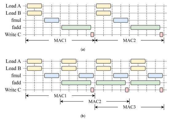
Figure 4.
The timing of multiply–accumulate (MAC) operations before (a) and after (b) applying pipelining.
4.2. Optimization for Constructing the M Matrix
In the original process of estimating pose using the EPnP algorithm, we need to construct a matrix M using 3D world coordinates and their 2D projections and store the matrix in RAM. After completing the process, the matrix M is then read from RAM and the product is calculated. The product is used to calculate eigenvectors in order to solve the PnP problem. This calculation process is very efficient for software. Unfortunately, for FPGA, the calculation of matrix M is a process that demands considerable time and resources. Matrix M is a matrix computed from each reference point. Due to the storage of reference points in floating-point format, with each number occupying 4 bytes of space, the matrix M occupies a total space of bytes. As the number of points increases, the size of the M matrix expands at a rate of two times, leading to an increase in the amount of RAM consumed. The proposed design supports a maximum of 512 reference points, thus requiring a reserved space of 48 KB for the M matrix. However, the total amount of RAM in FPGA is typically limited. This represents a significant resource overhead for FPGA.
There are two types of RAMs in FPGA: block RAM and distributed RAM. Distributed RAM typically has a smaller capacity but can achieve a larger bit width; block RAM has a larger capacity but a limited bit width. For the M matrix, which occupies a large amount of space, it is stored in block RAM. At this point, the read and write speed of the block RAM becomes a performance bottleneck for the system. Although the hardware circuits implemented by FPGA can be executed in parallel, the entire computation process is forced to be serial due to the necessity of serially writing data into BRAM, and then serially reading the data out of BRAM after the computation is completed. The calculation process hinders the effective implementation of pipelining, thereby diminishing the overall execution efficiency. Due to the significant time and hardware resource consumption required for computing the M matrix, optimizations targeting the calculation of the M matrix are necessary.
In this design, to optimize the computation process of matrix M, the construction and dot product calculations are considered as a whole, and the computation process is split up to bypass block RAM read and write operations as much as possible. As shown in Figure 5, instead of constructing the whole matrix M and then computing the product , we compute only one row of the M matrix each time. Multiplying this row vector by its transpose results in an intermediate matrix . Finally, by accumulating the intermediate matrices, the final result is obtained.
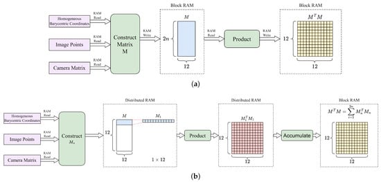
Figure 5.
The original (a) and optimized (b) calculation process of .
The result obtained through this calculation process is the same as that obtained from the original calculation process. On the one hand, the proposed calculation process eliminates the need to store the entire M matrix, which reduces the block RAM usage. On the other hand, since the intermediate matrix in the calculation process is stored in distributed RAM, which has a larger bit width than block RAM, the FPGA can perform pipelined computation more efficiently, thereby improving the calculation speed.
To validate the performance of the proposed computational method, we implemented two computation processes on FPGA and a comparative analysis of performance disparities was conducted between the two methods under identical input data conditions. Table 2 presents the experimental results. In the original computational process, it is necessary to retain the entire M matrix, resulting in the utilization of 32 block RAMs, which significantly impact storage requirements. Conversely, the proposed computational method saves storage space by eliminating the requirement to store the entire M matrix, marking a notable advancement in resource optimization. Due to the utilization of distributed RAM, the proposed computational process employs more Flip-Flops (FFs) and Lookup Tables (LUTs). When the number of points in the computational data is 512, the proposed computational method takes 57,391 clock cycles, whereas the original method consumes 595,120 clock cycles. By refining the computational process, a 10-fold acceleration in computation speed is achieved.
Table 2.
Resource utilization and speed comparison between the proposed calculation process and the original process.
4.3. Trade-Off between Speed and Area
The EPnP algorithm computes solutions for all four values of N. In theory, all four solutions can be calculated simultaneously to shorten the overall computing time, as shown in Figure 6a. While the computational speed has been accelerated, the implementation of four identical modules for Gauss–Newton optimization, pose calculation, and reprojection error computation has led to an increase in the consumption of hardware resources. Since the computing process takes a relatively short time, the design still adopts the serial computing method shown in Figure 6b. This allows for the reuse of hardware circuits, thereby reducing the consumed hardware resources.
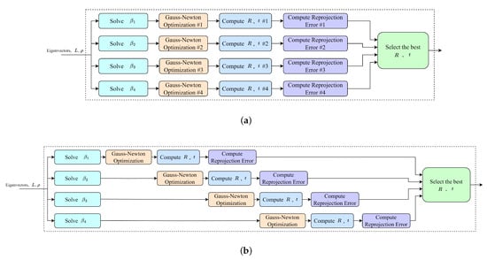
Figure 6.
Comparison between parallel computing (a) and pipeline computing (b).
5. Experimental Results
5.1. Accuracy and Speed Evaluation
In our experimental setup, we employ a predefined camera pose to project randomly generated world coordinate points onto a 2D plane, thereby obtaining the corresponding 2D projection points. In reality, due to the influence of noise, the 2D projection points will deviate within a certain range. In order to verify the system performance under the influence of noise, we applied Gaussian noise to each 2D projection point. We utilized the proposed PnP solution module to estimate the camera pose from these projections. At the same time, we used the solvePnP function in OpenCV as a benchmark to compare the differences in results between hardware and software implementations. OpenCV’s solvePnP method is a general approach used in computer vision projects to solve the PnP problem, and its default solver is also EPnP.
Figure 7 shows the accuracy performance of the proposed system. When no noise is introduced, the PSNR of the rotation matrix R exceeds 100 dB, while the displacement t achieves over 70 dB. At this point, the primary source of precision error lies in the accuracy of QR iteration for eigenvalue decomposition. In the presence of noise, the accuracy of the results decreases, and the PSNR value increases as the number of input points increases. At this point, the PSNR of the rotation matrix R can still be maintained at around 50 dB, with its accuracy slightly lower than that of OpenCV. This is due to the fewer iterations when solving for the eigenvectors. However, its accuracy can already satisfy most engineering requirements.
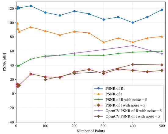
Figure 7.
PSNR performance of the proposed system and OpenCV with noise = 0, 5.
Figure 8 demonstrates the relationship between the number of calculation points and the computation time. The computation time grows linearly with the number of points, with a base value of 17.5 milliseconds.
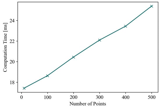
Figure 8.
The relationship between number of points and computation time.
5.2. Hardware Implementation
The PnP solver core is synthesized and implemented for Xilinx XC7K325T with Vivado HLS. The proposed system takes 1,473,295,500 clock cycles to complete computations for an input number of points of 300. In this system, the PnP algorithm is calculated in series, and the HLS tool will distribute the entire calculation process evenly to each clock cycle. While meeting the timing requirements, it tries to shorten the number of clock cycles as much as possible. Therefore, the clock frequency of FPGA has little impact on the total time of a single calculation. After actual testing, a higher clock frequency cannot bring a shorter total calculation time. Upon comprehensive consideration, a clock frequency of 67 MHz has been deliberately selected for the FPGA implementation. Therefore, the total calculation time is 22.1 ms. The hardware resource utilization of the prototype system is reported in Table 3.
Table 3.
FPGA resource utilization of the proposed system.
5.3. Power Efficiency Comparison
We implemented the same algorithm on several computing platforms and measured the computational time consumed. To measure the actual operational power consumption of the system, we downloaded the FPGA implementation mentioned above onto a Kintex-7 Base board. The Kintex-7 Base board is equipped with a Xilinx XC7K325T-FFG676 FPGA. During the testing process, the FPGA cyclically performs PnP calculations for 300 input data points, which allows us to calculate the average power consumption of the system based on its total power consumption over a period of time. Since the Kintex-7 Base board is powered by USB, we inserted a USB power meter between the power adapter and the board to record the electricity consumed by the board over one minute. The same method was used to test the power consumption of the ZYNQ processor. A program that repeatedly executes the PnP solution algorithm is downloaded onto a XC7Z010 board, and the average power consumption is measured using the USB power meter. To measure the execution time of the PnP algorithm on the Zynq-7000 processor, another experiment was conducted. The system timer of the Zynq-7000 was used to measure the time required for the program to execute from start to finish, and the results were sent to the host computer via a serial port.
For desktop-level processors, their power consumption can be measured by sensors on the motherboard. We used CoreTemp software to read the overall package power consumption of the processor. Due to the presence of the operating system, the processor consumes power even when it is not executing the PnP solution task, so we measured the power consumption of the processor during both idle and execution states and took the difference as the power consumption of the PnP solution.
Table 4 shows the comparison of calculation time and speed of the PnP solution algorithm on different platforms. Despite the relatively high resource utilization rate of this design, the power is still only 1.7 W. There are two main reasons for achieving such low power consumption: Firstly, the operation of an algorithm requires the implementation of both computational and control circuits. The operation process of FPGA is a state machine, which consumes most of its energy on computation, while control only consumes a small portion of the power. Unlike FPGA, CPUs consume a large amount of power on fetching and decoding instructions during computation, with only a small part of the power consumption used for actual computation. Therefore, its energy efficiency is much lower than that of FPGA. Secondly, the proposed PnP calculation process on FPGA runs in series. When a part of the FPGA circuit is calculating, the rest of the parts are inactive. This allows FPGA to have lower power consumption per unit time. However, the disadvantage of this approach is that FPGA does not fully utilize its hardware in terms of time, resulting in the consumption of more resources and also leading to slower computation speeds.
Table 4.
Speed and power comparison.
Although the FPGA implementation is slightly slower than the X86 processor in terms of speed, each computational iteration consumes merely 3.9% of the electric energy consumed by the aforementioned method, demonstrating substantial energy efficiency. When solving the PnP problem on battery-powered computing devices, higher energy efficiency leads to longer working hours, making it suitable to be applied to robotics and VR headsets. At the same time, the FPGA implementation exhibits significantly enhanced processing speeds in comparison to the ARM-based application processor. FPGA achieves faster computing speed while consuming only 43.4% of the energy of the latter. FPGA can achieve real-time data processing at 45.2 fps, which is important for computer vision tasks.
6. Conclusions
This paper proposes an energy-efficient Perspective-n-Point accelerator implemented on FPGA. The solver core implements a basic matrix operation library, as well as eigenvalue and eigenvector solvers and linear least squares equation solvers based on QR decomposition. On this basis, the computational process of the EPnP algorithm is implemented. By using hardware pipelining and adjusting the calculation order of the algorithm, the computation speed is improved while reducing hardware resource consumption. The proposed design not only meets the requirement for real-time computation, but it is also more efficient compared to other computing hardware. The advantages of this design make it suitable to be applied to mobile robots and other situations that require low power consumption.
Future research can be carried out in the following areas. (1) In the hardware PnP solver proposed in this design, all data are calculated and stored using single-precision floating-point numbers. Fixed-point numbers offer faster computation speeds compared to floating-point numbers while also occupying fewer FPGA resources. Therefore, replacing floating-point numbers with fixed-point numbers for PnP solution can be explored, and the impact of this operation should be evaluated. (2) In the EPnP algorithm, due to the interdependence of data, the same set of data may be used at different stages of the computation. When the computation of the current sequence is completed, the data still need to be stored in RAM, occupying storage space and preventing the next set of data from starting its computation. In this design, only after a round of PnP solution is completed can the next set of data begin computation, which reduces the utilization rate of hardware resources. To address this, pipelining optimization can be applied throughout the design to reduce the initiation interval and improve throughput. (3) Parallel QR decomposition algorithms can be studied to reduce the latency of the design.
Author Contributions
Conceptualization, methodology, developing, testing and writing—original draft preparation, H.L.; writing—review and editing, supervision, Q.W. All authors have read and agreed to the published version of the manuscript.
Funding
This research received no external funding.
Data Availability Statement
Data are contained within the article.
Conflicts of Interest
The authors declare no conflicts of interest.
Abbreviations
The following abbreviations are used in this manuscript:
| FPGA | Field-Programmable Gate Array |
| PnP | Perspective-n-Point |
| HLS | High-level Synthesis |
| SLAM | Simultaneous Localization and Mapping |
| VR | Virtual Reality |
| RTL | Register Transfer Level |
| QRD | QR Decomposition |
| DLT | Direct Linear Transformation |
| RAM | Random Access Memory |
| BRAM | Block Random Access Memory |
| CORDIC | Coordinate Rotation Digital Computer |
| PSNR | Peak Signal To Noise Ratio |
| MSE | Mean Squared Error |
| DSP | Digital Signal Processor |
| FF | Flip-Flop |
| LUT | Look-Up Table |
| MAC | multiply–accumulate |
References
- Lepetit, V.; Moreno-Noguer, F.; Fua, P. EPnP: An Accurate O(n) Solution to the PnP Problem. Int. J. Comput. Vis. 2009, 81, 155–166. [Google Scholar] [CrossRef]
- Cui, T.; Guo, C.; Liu, Y.; Tian, Z. Precise Landing Control of UAV Based on Binocular Visual SLAM. In Proceedings of the 2021 4th International Conference on Intelligent Autonomous Systems (ICoIAS), Wuhan, China, 14–16 May 2021; pp. 312–317. [Google Scholar]
- Li, W.; Li, D.; Shao, H.; Xu, Y. An RGBD-SLAM with Bi-Directional PnP Method and Fuzzy Frame Detection Module. In Proceedings of the 2019 12th Asian Control Conference (ASCC), Kitakyushu, Japan, 9–12 June 2019; pp. 1530–1535. [Google Scholar]
- Zhou, M.; Li, S.; Lu, W. An Improved SLAM Based On The Indoor Mobile Robot. In Proceedings of the 2022 34th Chinese Control and Decision Conference (CCDC), Hefei, China, 15–17 August 2022; pp. 5594–5601. [Google Scholar]
- Zhou, H.; Zhang, T.; Jagadeesan, J. Re-Weighting and 1-Point RANSAC-Based PnnP Solution to Handle Outliers. IEEE Trans. Pattern Anal. Mach. Intell. 2019, 41, 3022–3033. [Google Scholar] [CrossRef] [PubMed]
- Cong, J.; Liu, B.; Neuendorffer, S.; Noguera, J.; Vissers, K.; Zhang, Z. High-Level Synthesis for FPGAs: From Prototyping to Deployment. IEEE Trans.-Comput.-Aided Des. Integr. Circuits Syst. 2011, 30, 473–491. [Google Scholar] [CrossRef]
- Nane, R.; Sima, V.-M.; Pilato, C.; Choi, J.; Fort, B.; Canis, A.; Chen, Y.T.; Hsiao, H.; Brown, S.; Ferrandi, F.; et al. A Survey and Evaluation of FPGA High-Level Synthesis Tools. IEEE Trans.-Comput.-Aided Des. Integr. Circuits Syst. 2016, 35, 1591–1604. [Google Scholar] [CrossRef]
- Fischler, M.A.; Bolles, R.C. Random Sample Consensus: A Paradigm for Model Fitting with Applications to Image Analysis and Automated Cartography. In Readings in Computer Vision; Fischler, M.A., Firschein, O., Eds.; Morgan Kaufmann: San Francisco, CA, USA, 1987; pp. 726–740. ISBN 978-0-08-051581-6. [Google Scholar]
- Zeng, G.; Chen, S.; Mu, B.; Shi, G.; Wu, J. CPnP: Consistent Pose Estimator for Perspective-n-Point Problem with Bias Elimination. In Proceedings of the 2023 IEEE International Conference on Robotics and Automation (ICRA), London, UK, 29 May–2 June 2023; pp. 1940–1946. [Google Scholar]
- Pan, S.; Wang, X. A Survey on Perspective-n-Point Problem. In Proceedings of the 2021 40th Chinese Control Conference (CCC), Shanghai, China, 26–28 July 2021; pp. 2396–2401. [Google Scholar]
- Lu, C.-P.; Hager, G.D.; Mjolsness, E. Fast and Globally Convergent Pose Estimation from Video Images. IEEE Trans. Pattern Anal. Mach. Intell. 2000, 22, 610–622. [Google Scholar] [CrossRef]
- Horaud, R.; Dornaika, F.; Lamiroy, B. Object Pose: The Link between Weak Perspective, Paraperspective, and Full Perspective. Int. J. Comput. Vis. 1997, 22, 173–189. [Google Scholar] [CrossRef]
- Abdel-Aziz, Y.I.; Karara, H.M.; Hauck, M. Direct Linear Transformation from Comparator Coordinates into Object Space Coordinates in Close-Range Photogrammetry. Photogramm. Eng. Remote Sens. 2015, 81, 103–107. [Google Scholar] [CrossRef]
- Fiore, P.D. Efficient Linear Solution of Exterior Orientation. IEEE Trans. Pattern Anal. Mach. Intell. 2001, 23, 140–148. [Google Scholar] [CrossRef]
- Quan, L.; Lan, Z. Linear N-Point Camera Pose Determination. IEEE Trans. Pattern Anal. Mach. Intell. 1999, 21, 774–780. [Google Scholar] [CrossRef]
- Ansar, A.; Daniilidis, K. Linear Pose Estimation from Points or Lines. IEEE Trans. Pattern Anal. Mach.-Intel-Ligence 2003, 25, 578–589. [Google Scholar] [CrossRef]
- Eigen. Available online: https://eigen.tuxfamily.org/index.php?title=Main_Page (accessed on 24 September 2024).
- Zhao, W.; Li, C.; Ji, Z.; Guo, Z.; Chen, X.; You, Y.; Huang, Y.; You, X.; Zhang, C. Flexible High-Level Synthesis Library for Linear Transformations. IEEE Trans. Circuits Syst. II Express Briefs 2024, 71, 3348–3352. [Google Scholar] [CrossRef]
- Venkata Siva Kumar, K.; Kopparthi, V.R.; Sabat, S.L.; Varma., K.T.; Peesapati, R. System on Chip Implementation of Floating Point Matrix Inversion Using Modified Gram–Schmidt Based QR Decomposition on PYNQ FPGA. In Proceedings of the 2021 IEEE International Symposium on Smart Electronic Systems (iSES), Jaipur, India, 18–22 December 2021; pp. 84–88. [Google Scholar]
- Golub, G.H.; Loan, C.F.V. Matrix Computations; JHU Press: Baltimore, MD, USA, 2013; ISBN 978-1-4214-0859-0. [Google Scholar]
- Omran, S.S.; Abdul-abbas, A.K. Design and Implementation of 32-Bits MIPS Processor to Perform QRD Based on FPGA. In Proceedings of the 2018 International Conference on Engineering Technology and their Applications (IICETA), Al-Najaf, Iraq, 8–9 May 2018; pp. 36–41. [Google Scholar]
- Aslan, S.; Niu, S.; Saniie, J. FPGA Implementation of Fast QR Decomposition Based on Givens Rotation. In Proceedings of the 2012 IEEE 55th International Midwest Symposium on Circuits and Systems (MWSCAS), Boise, ID, USA, 5–8 August 2012; pp. 470–473. [Google Scholar]
- Tan, C.Y.; Ooi, C.Y.; Ismail, N. Loop Optimizations of MGS-QRD Algorithm for FPGA High-Level Synthesis. In Proceedings of the 2019 32nd IEEE International System-on-Chip Conference (SOCC), Singapore, 3–6 September 2019; pp. 138–143. [Google Scholar]
- Lee, D.; Hagiescu, A.; Pritsker, D. Large-Scale and High-Throughput QR Decomposition on an FPGA. In Proceedings of the 2019 IEEE 27th Annual International Symposium on Field-Programmable Custom Computing Machines (FCCM), San Diego, CA, USA, 28 April–1 May 2019; p. 337. [Google Scholar]
Disclaimer/Publisher’s Note: The statements, opinions and data contained in all publications are solely those of the individual author(s) and contributor(s) and not of MDPI and/or the editor(s). MDPI and/or the editor(s) disclaim responsibility for any injury to people or property resulting from any ideas, methods, instructions or products referred to in the content. |
© 2024 by the authors. Licensee MDPI, Basel, Switzerland. This article is an open access article distributed under the terms and conditions of the Creative Commons Attribution (CC BY) license (https://creativecommons.org/licenses/by/4.0/).