Lightweight Bearing Fault Diagnosis Method Based on Improved Residual Network

Abstract

A lightweight bearing fault detection approach based on an improved residual network is presented to solve the shortcomings of previous fault diagnostic methods, such as inadequate feature extraction and an excessive computational cost due to high model complexity. First, the raw data are turned into a time–frequency map using the continuous wavelet transform, which captures all of the signal’s time- and frequency-domain properties. Second, an improved residual network model was built, which incorporates the criss-cross attention mechanism and depth-separable convolution into the residual network structure to realize the important distinction of the extracted features and reduce computational resources while ensuring diagnostic accuracy; simultaneously, the Meta-Acon activation function was introduced to improve the network’s self-adaptive characterization ability. The study findings indicate that the suggested approach had a 99.95% accuracy rate and a floating point computational complexity of 0.53 GF. Compared with other networks, it had greater fault detection accuracy and stronger generalization ability, and it could perform high-precision fault diagnostic jobs due to its lower complexity.

1. Introduction

Rolling bearings are important bearing parts of generators, turbines, compressors, aviation generators, and other rotating machinery. Their own physical state is related to the operation of the entire production equipment. Due to its high load in harsh conditions for a long running time, they are very prone to a variety of failures. According to statistics on machinery and equipment, about 30% of equipment failures are due to bearing damage. Therefore, the diagnosis of rolling bearings is highly essential [1,2].

Nowadays, more and more scholars have used the deep learning method with powerful feature extraction capability and good adaptability in rotating machinery fault identification, and many results were achieved [3,4,5]. A convolutional neural network (CNN) [6], as a typical deep learning method, can automatically extract abstract characteristics and categorize them with strong characterization abilities, and it has been a study focus in the field of defect diagnosis. Jans et al. [7] were the first to successfully use a convolutional neural network to diagnose faults in bearings and gearboxes. Fu et al. [8] proposed a two-dimensional time–frequency image extended with labeled fault data using data-enhancement techniques that was input into a CNN for fault diagnosis. Wang et al. [9] presented a deep fusion of multi-source information based on a deep residual convolutional neural network for rolling bearing failure detection. Neupane et al. [10] proposed a switchable normalization-based convolutional neural network (SN-CNN)-based fault diagnosis. Irfan et al. [11] proposed a weighted voting ensemble (WVE) of three low-computation custom-designed convolutional neural networks (CNNs) to classify bearing faults. Hao et al. [12] proposed replacing the classic ResNet’s fully connected layer with the global average pooling (GAP) approach to increase the fault identification accuracy. Song et al. [13] used the approach of broadening the convolutional kernel to generate a bigger sensory field, and they created a convolutional neural network (WKCNN) model with a wide convolutional kernel for quick feature extraction. The diagnostic model presented by the aforementioned technique is resilient and accurate, but it cannot dynamically modify the level of attention to characteristics based on varied input data.

To extract richer and more comprehensive fault features and improve the generalization and diagnostic accuracy of the model, Plakias et al. [14] proposed focused dense convolutional neural networks (ADCNNs), which combine dense convolutional blocks with attention mechanisms. Wang et al. [15] improved the residual network by using soft thresholding and pyramid compression attention to filter background noise and learn richer multi-scale feature information to increase the defect diagnosis rates. Chen et al. [16] proposed improving the image quality by using a dense residual module and a two-stream attention module to improve the network adaptability, as well as enhancing some important features with the help of a two-stream attention module to focus on basic visual features. Wang et al. [17] developed a transferable convolutional neural network (TCNN) with five convolutional modules to improve target task learning. Saghi et al. [18] proposed a multi-scale CNN method. This method extracts the spatial and temporal features of various vibration signals at different scales, combines them, and classifies them. Yu et al. [19] combined ResNet and SAM networks to create a deep feature extraction network capable of extracting both local and global time–frequency data. Karnavas et al. [20] proposed attention stream networks, which are generated by the connection of two independent neural streams and can produce features with different characteristics in parallel. Ren et al. [21] input the time-domain data and the original signal into two CNN branches, and the multi-head self-attention (MS) mechanism adaptively aggregated and weighted the features recovered by the CNN.

However, the above methods primarily focus on changing the network structure and constructing a deep network with a complex structure to solve the loss of features between layers and the influence of shallow features on deep features. Although the ability to express features is strong and the diagnostic performance, generalization performance, etc., of the resultant network is improved, the number of parameters and the amount of computation are huge, which result in high computational costs. This research presents a lightweight defect diagnostic approach for bearings using an upgraded residual network to address the issues mentioned above. The model enhances the residual network characterization with CCA, decreases the computational costs with depth-separable convolution, and improves the network correctness with Meta-Acon activation. Compared with existing models, the model suggested in this study offers significant improvements in both feature representation capability and fault diagnosis accuracy while remaining lightweight.

2. Theoretical Foundation

2.1. Continuous Wavelet Transform

The continuous wavelet transform (CWT) can acquire the signal’s local characteristics using wavelet functions of different scales and positions while also providing time and frequency information [22], which makes it well suited to non-stationary signals. CWT is used to transform the bearing’s one-dimensional vibration time-domain signal into a two-dimensional time–frequency diagram, which can more accurately and comprehensively depict the signal features [23].

The CWT definition is expressed as follows:

$$W_f(a,\tau )={\displaystyle \frac{1}{\sqrt{\left|a\right|}}}{\displaystyle {\int }_{-\infty }^{\infty }f(t){\phi }^{\ast }(\frac{t-\tau }{a})}dt$$

(1)

The parameter $f(t)$ is the input signal; ${\phi }^{\ast }(t)$ denotes the complex conjugate of $\phi (t)$; ${\phi }_{a,\tau }(t)$ is the basis function of the continuous wavelet; and $a$ is the scale factor and $\tau$ is the translation factor, which control the scaling and translation of the wavelet function, respectively.

The two-dimensional picture data fit better with the deep convolutional neural net-work model. In this study, the continuous wavelet transform was employed to convert one-dimensional bearing vibration data into two-dimensional time–frequency pictures that are fed into the improved residual network model for processing.

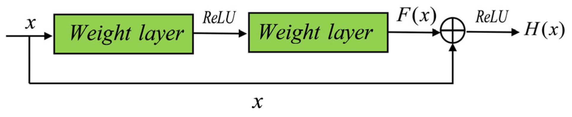
2.2. Residual Networks

Residual networks use constant pathways to simplify parameter optimization [24], which addresses the issue of vanishing gradients in deep networks by building the network with residual blocks as its basic units, as illustrated in Figure 1.

Each residual block in the graphic consists of two convolutional layers and a cross-layer connection. The cross-layer connection adds the inputs directly to the outputs, and the residual operation is expressed as follows:

$$H(x)=x+F(x,w_t)$$

(2)

The parameter $F(x)$ is the residual function, x is the input, $w_t$ is the weight corresponding to the input value, and $H(x)$ is the output. ResNet can learn the fluctuations of the residuals by introducing the residual module, which allows it to capture more information and features in a picture. In addition, jump connections help to lessen gradient vanishing and gradient explosion issues, which makes the network easier to train. The DARB module proposed in this paper is built on this structure.

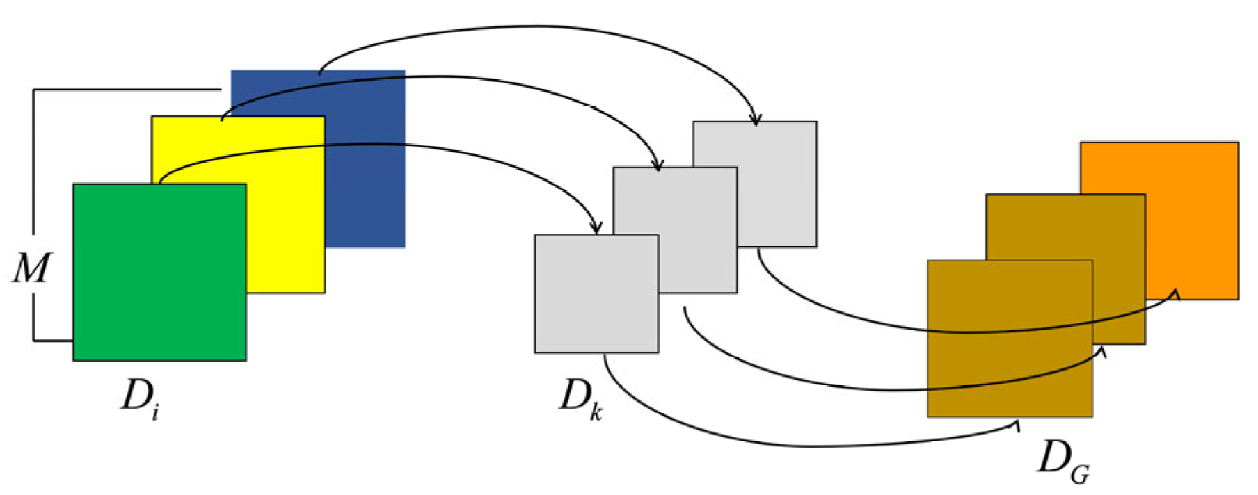
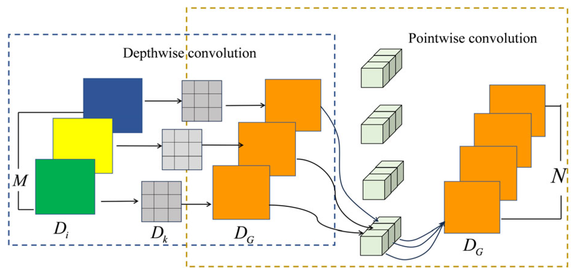
2.3. Depth-Separable Convolution

Depth-separable convolution is composed of two parts: depthwise convolution and pointwise convolution [25]. Figure 2 and Figure 3 depict the ordinary convolution and depth-separable convolution processes, respectively. The input data size is $D_i\times D_i\times M$ and the convolution kernel is $D_k\times D_k\times M\times N$. The following equation shows the ratio of parametric values between depth-separable convolution and traditional convolution:

$${\displaystyle \frac{D_i\times D_i\times M\times D_k\times D_k+D_i\times D_i\times M\times N}{D_i\times D_i\times M\times N\times D_k\times D_k}}={\displaystyle \frac{1}{N}}+{\displaystyle \frac{1}{D_k^2}}$$

(3)

As can be seen, the number of deeply separable parameters is ${\displaystyle \frac{1}{N}}+{\displaystyle \frac{1}{D_k^2}}$ times that of the ordinary convolution, the number of parameters is lower, and the computational amount is smaller. This paper proposes using DSC instead of traditional convolution in residual networks to improve the model structure, training speed, and accuracy.

2.4. Criss-Cross Attention

Criss-cross attention (CCA) [26] can be used to extract key features in bearing vibration signals and improve the accuracy and efficiency of fault diagnosis by introducing two crossing paths, i.e., horizontal and vertical paths, to capture correlation information between different locations in the feature map and adopting the “criss-cross” computation method to reduce the number of network parameters, which does not take up too much memory and computational resources. Figure 4 illustrates the network structure of CCA.

CCA obtains the corresponding attention matrix by performing a 1 × 1 convolution operation on the input feature map to the feature maps of query, key, and value for each position $u$, where it first extracts the feature vectors of the pixel positions that are in the same row or column as its counterparts from the key feature map ${\Omega }_u$, and then computes the similarity of $Q$ and $K$ using affinity:

$$d_{i,u}=Q_u{\Omega }_{i,u}^{ T}$$

(4)

The parameter $d_{i,u}\in D$ denotes the degree of correlation between the features $Q_u$ and ${\Omega }_{i,u}$, where $i=[1,\dots ,\left|{\Omega }_u\right|]$.

The softmax operation is used to obtain the positional attention weights $A\in R^{(H+W-1)\times W\times H}$, $H+W-1$ vectors from the final feature map $V\in R^{C\times W\times H}$ that are in the same row or column as the position are extracted to form the vector set ${\Phi }_u\in R^{(H+W-1)\times C}$, and the aggregation operation is used to obtain the feature vectors of the output feature map $H\prime \in {\mathrm{R}}^{\mathrm{C}\times \mathrm{W}\times \mathrm{H}}$ at position $u$. The feature vectors of the output feature map at position u are obtained through the aggregation operation.

$$H_u^{\prime }={\displaystyle \sum _{i\in \left|{\Phi }_u\right|}{A}_{i,u}{\Phi }_{i,u}+H_u}$$

(5)

The parameter $A_{i,u}$ is the scalar value at channel $i$ and location $u$.

The CCA module improves the network’s ability to interact with time–frequency images across channels and space. It captures feature information from cross-paths and surrounding pixels, which improves the model’s perception of global features and fault classification accuracy.

2.5. Adaptive Activation Function Meta-Acon

The typical activation function ReLU has become a more frequent activation function due to its wonderful characteristics, such as non-saturation and sparsity. However, it is susceptible to gradient expansion and neuron “necrosis”. To compensate for the activation function’s shortcomings, this paper introduces a new activation function, Meta-Acon, that adaptively adjusts whether or not to activate neurons to better adapt to different data distributions, thereby improving the model’s generalizability [27].

The Meta-Acon activation function is calculated as shown in Equation (6):

$$F(x)=(p_1-p_2)x\times \delta (\beta (p_1-p_2)x)+p_{2}x$$

(6)

The parameter $\delta$ denotes the sigmoid function; $p_1$ and $p_2$ are learnable parameters.

The Meta-Acon activation function improves on the ReLU and Swish activation functions by introducing a dynamic learning and control mechanism. This mechanism sets the value produced by the two-layer 1 × 1 convolution to determine whether a neuron $\beta$ is activated or not. This network uses a channel-level architecture, where components in a channel share the same parameter $\beta$. The formulation’s $\beta$ parameter determines whether neuron activation is linear or nonlinear.

The adaptive function $\beta$ is shown in Equation (7), which is first averaged for the $h$ and $w$ dimensions, respectively; second, it goes through two convolutional layers, $W_1$ and $W_2$, so that all the pixels in each channel share a single weight; finally, $\beta$ is derived from the sigmoid function, where $\delta$ denotes the sigmoid function:

$$\beta =\delta W_1{W}_2{\displaystyle \sum _{h=1}^H{\displaystyle \sum _{w=1}^{W}x,h,w}}$$

(7)

The parameters $W_1\in R^{c\times c/r}$ and $W_2\in R^{c/r\times c}$. The first $c$ in $W_1$ is the dimension of the input and $c/r$ is the dimension of the output; the first $c/r$ in $W_2$ is the dimension of the input, $c$ is the dimension of the output, and $r$ is the scaling factor, which is usually taken to be 2$n$ and was set to 16 in this network.

3. Improved Residual Network

3.1. Residual Block

Combining the advantages of residual networks and attention mechanisms in image classification and feature extraction, the network’s basic module introduces the residual module to solve the problem of gradient disappearance and network degradation, which was inspired by SARN [28]. By adding channel attention weights to the jump connections of the residual module, it can preserve and enhance key information during the transmission process. Adding attention to the main branch of the residual module allows the model to pay more attention to key features when extracting features, which improves the model’s feature extraction ability, makes the extracted features more accurate and effective, and ultimately achieves the goal of improving the residual network’s overall performance. The CCA mechanism considerably improves the model’s capacity to pay attention to critical information. This attention method applies learnable weights to various feature maps and highlights the relevant feature maps, hence improving the model’s perception of the features and feature representation abilities. Replacing standard convolution in the residual module with depth-separable convolution can eliminate duplicate information while reducing the number of model parameters and computations. The Meta-Acon activation function is used to regulate the degree of nonlinearity in each layer of the network, which considerably improves the model performance and computational correctness. The specific structure is depicted in Figure 5.

3.2. Model Building

Based on the preceding theory and the network base module, the lightweight bearing fault diagnosis model framework based on the improved residual network was established, and the network structure is shown in Figure 6, which includes a convolution layer, a pooling layer, an improved residual module, and a fully connected layer. First, the continuous wavelet transform is employed to generate a time–frequency map of the vibration data, which is then fed into the model. Convolution is then used to extract the shallow edge features of the time–frequency map, while the Meta-Acon activation function allows the network to adaptively activate, and maximum pooling retains the data’s key properties. Second, stacked residual modules are used to learn richer and more discriminative features, which improve feature extraction and representation. Finally, the feature map is compressed by global average pooling, and dropout is added between two full connections to reduce the co-adaptation between neurons. This improves the model generalization ability, suppresses overfitting, and implements fault diagnosis by using the softmax layer as a classifier.

Table 1. Network structure parameters.

Layer		Convolution Kernel	Input and Output Dimensions
Input		-	3 × 64 × 64
Conv		16 × 16	128 × 55 × 55
BN Meta-Acon		-	128 × 55 × 55
Maxpool		2 × 2	128 × 28 × 28
Residual block 1	Criss-cross attention	-	128 × 28 × 28
	DSCconv	3 × 3	128 × 28 × 28
	BN Meta-Acon	-	128 × 28 × 28
	DSCconv	3 × 3	128 × 28 × 28
	BN	-	128 × 28 × 28
Meta-Acon		-	128 × 28 × 28
Maxpool		2 × 2	128 × 15 × 15
Residual block 2	Criss-cross attention	-	128 × 15 × 15
	DSCconv	3 × 3	128 × 15 × 15
	BN Meta-Acon	-	128 × 15 × 15
	DSCconv	3 × 3	128 × 15 × 15
	BN	-	128 × 15 × 15
Avgpool		-	128 × 1 × 1
Fc		-	256
Softmax		-	10

displays various network structure parameters.

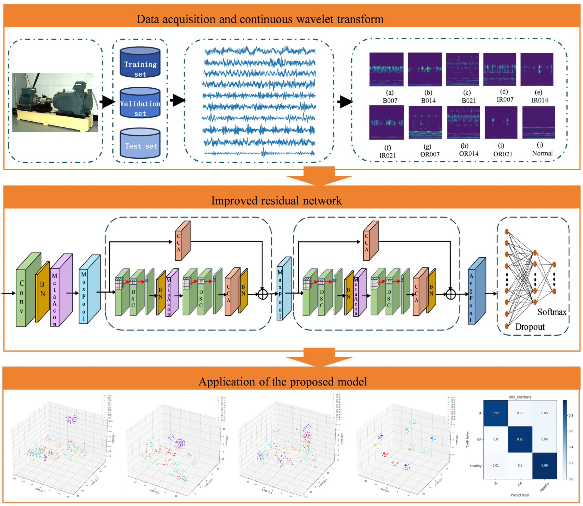
3.3. Fault Diagnosis Process

Figure 7 depicts the flow chart for the lightweight bearing failure diagnostic technique based on an improved residual network. The particular stages are as follows:

• Data processing: obtain the vibration signal, convert it to a time–frequency map after overlapping sampling to increase the number of samples using the continuous wavelet transform, and then convert the one-dimensional vibration signal to a two-dimensional time–frequency map.
• Model training: load the training set samples into the improved residual network for training and configure the network structure parameters, the maximum number of iterations of the loss function, and the number of training iterations.
• Model validation: Save the trained lightweight model, validate it using test set samples, and output the diagnosis findings. Use accuracy, precision, and recall as assessment metrics.

4. Experimental Validation

4.1. Data Description

This work used experimental validation with the Case Western Reserve University (CWRU) [29] bearing dataset and the Paderborn University (PU) [30] bearing dataset.

4.1.1. CWRU Bearing Failure Dataset

The experimental data used in this article are the driving end data from the CWRU bearing defect data collection. The sample frequency was 12 kHz, and EDM was used to organize single-point damage in the outer ring, inner ring, and rolling body of the bearings, with each defect having three damage diameters of 0.178 mm, 0.356 mm, and 0.533 mm. The experimental data for comparison included vibration signals from these nine types of bearing failures recorded at loads of 0, 1, 2, and 3 HP (rotational speeds of 1797, 1772, 1750, and 1730 r/min), as well as normal vibration signals. To increase the number of samples, data improvement was performed using overlapping samples to obtain 1024 data points as a sample, and the experimental samples were separated as indicated in

Table 2. Experimental datasets of CWRU.

Load	Fault Type	Fault Diameter/mm	Training/Validation/Test Set	Tags
0/1/2/3 HP	Normal	0	800/100/100	0
	Inner-ring fault	0.178	800/100/100	1
		0.356	800/100/100	2
		0.533	800/100/100	3
	Outer-ring failure	0.178	800/100/100	4
		0.356	800/100/100	5
		0.533	800/100/100	6
	Rolling body failure	0.178	800/100/100	7
		0.356	800/100/100	8
		0.533	800/100/100	9

. The data samples were divided in an 8:1:1 ratio and labeled. They were utilized for training the model, as well as validating and testing its effectiveness.

4.1.2. PU Bearing Failure Dataset

The PU dataset [30] is a public dataset published by Christian Lessmeier et al. of Padburn University PU, Germany, and includes healthy, man-made, and natural damage data. Figure 8 depicts the data collection experimental bench for the PU dataset, which includes a motor, torque-measuring shaft, bearing, test module, flywheel, and load motor from left to right. The test bearings set involved the test module, flywheel, and load motor, and all of them contained 6203 rolling bearings. Piezoelectric acceleration sensors were utilized to capture vibration data from the base of the bearings during operations, with a sample frequency of 64 kHz.

The sub-dataset utilized in this article comprised data from the bearing experimental platform at a drive system speed of 1500 rpm, a load torque of 0.1 Nm, and a radial force of 1000 N. Signals from 18 sets of bearings were selected, including 6 sets each for inner-ring faults, healthy outer-ring faults, and healthy bearings, which covered all of the faults that were really damaged in the dataset, which made it convenient to test the approach described in this study. The data utilized in this paper’s studies were likewise overlapped samples with a sample length of 1024; there were 2400 samples for each defect type, which were separated into a training set, a validation set, and a test set with an 8:1:1 ratio, as shown in

Table 3. Experimental datasets of PU.

Fault Type	Tags	Bearing Number	Training/Validation/Test Set
Inner-ring failure	0	KI01, KI05, KI07, KI14, KI16, KI17	1920/240/240
Outer-ring failure	1	KA01, KA05, KA07, KA04, KA15, KA16	1920/240/240
Healthy	2	K001, K002, K003, K004, K005, K006	1920/240/240

.

4.2. Experimental Setup

The simulation tests in this study were based on the Linux operating system, an Intel (R) Xeon (R) Gold 6148 CPU (Intel Corporation, Santa Clara, CA, USA), 512 GB of RAM, and an NVIDIA A40 GPU (Nvidia Corporation, Santa Clara, CA, USA) for graphics. The network model was built using the deep learning framework Pytorch 1.12 and configured with the Python 3.8 programming language.

The original one-dimensional fault signal was transformed into a two-dimensional time–frequency diagram using a continuous wavelet transform, and one diagram was chosen for each of the four fault states to display, as shown in Figure 9. The input image size was set to 64 × 64; the batch size was 32; the number of iterations was 35; MSE was used as the error loss function; Adam was the optimizer; and the learning rate was 0.001, where the learning rate was adjusted by using the learning rate decay mechanism (StepLR), and the learning rate was halved for every ten iterations to improve the training effect and reduce the cost of training time.

4.3. Evaluation Indicators

Accuracy, parameters, and FLOPs were used to evaluate the model’s overall performance. The parameter count specifies the number of parameters that may be trained in the network model, and FLOPs are the number of floating point operations; the higher the FLOPs, the more complicated the model. The recognition accuracy $A_C$ is calculated as follows:

$$A_C={\displaystyle \frac{P_r}{P_a}}\times 100\%$$

(8)

The parameter $P_r$ denotes the number of samples where the fault type was correctly predicted and $P_a$ denotes the number of samples for the fault type overall.

4.4. Analysis of Experimental Results on the CWRU Dataset

4.4.1. Ablation Experiments

This section describes a set of ablation experiments that assessed the impact of including DSC, CCA, and Meta-Acon modules into the residual network on the network recognition performance.

Table 4. Comparison of mixed-load data-centralized ablation experiments.

Network Model	Mixed-Load Datasets
	Accuracy/%	Precision/%	Recall/%	AUC/%
Basic model	93.52	94.2	93.41	99.42
Basic model + DSC	93.7	94.51	93.6	99.42
Basic model + CCA	95.94	95.78	95.84	99.63
Basic model + DSC + CCA	99.82	96.62	96.49	96.88
Improved residual network	99.95	96.64	96.53	99.74

shows the results of the ablation experiments performed by adding the DSC and CCA modules and replacing the ReLU activation function with Meta-Acon.

Table 4 compares the effects of the DSC, CCA, and Meta-Acon modules introduced in this paper in terms of the network recognition performance, and it can be seen that each module had a positive facilitating effect on the bearing fault diagnosis, and the introduction of the CCA made the indicators of accuracy, precision, and recall rise significantly compared with the baseline network, which was due to the fact that the CCA could combine feature input from multiple locations to provide more representative feature representations, and hence, improve the network’s capacity to filter information during the learning process. Using the adaptive Meta-Acon function improved the model’s performance by learning when to activate a neuron. The experimental results demonstrate that the network design method described in this study was beneficial.

4.4.2. Model Complexity Experiments

In the realm of bearing defect detection, theoretically, increasing the depth of the network structure typically improves the model’s capacity to extract complicated information, which results in lower prediction errors and higher diagnostic accuracy. However, when the network complexity increases, gradient difficulties (gradient disappearing or gradient explosion) and a large waste of computer resources may arise. As a result, while deciding how many network layers to use, model performance, computational complexity, and other multi-objective optimization must all be considered. In this study, we created three distinct depths of the residual structure, i.e., the number of residual modules were one, two, or three, and we performed tests on each of the different depths of the network structure, where the statistical test results are shown in

Table 5. Model complexity experiments.

Number of Residual Blocks	Params/M	FLOPs/GF	Accuracy/%
One	0.38	0.45	95.32
Two	0.53	0.49	99.95
Three	0.73	0.52	99.96

.

The recognition accuracy increased as the network depth increased, but the number of parameters and number of floating-point computations improved by 37.74% and 6.12%, respectively, when the network model used three residual blocks versus two residual blocks, while the accuracy improved by only 0.01%. After thorough research, this study concluded that using two residual blocks in the network model may effectively equalize the performance and computational cost.

4.4.3. Single-Load Scenario Experiments

To demonstrate the efficiency of the lightweight bearing defect diagnostic technique based on the improved residual network, several current mainstream network models in the field of deep learning were selected: ResNet18; ResNet50; VGG16; Swin Transformer (Swin-T) [31]; two representative lightweight CNN architectures, namely, MobileNetV2 [32] and ShuffleNetV2 [33]; and the upgraded ECA_ResNet [34] were tested and compared. The number of network parameters, the floating-point computation volume, and the diagnostic accuracy were used as diagnostic effect evaluation indexes, and the experimental results are shown in

Table 6. Accuracy of different methods under single load.

Network Method	Params/MB	FLOPs/GF	Accuracy/%
ShuffleNetV2	1.26	0.23	99.26
MobileNetV2	2.3	0.39	99.43
VGG16	264	4.87	98.70
ResNet18	22	0.69	99.78
ResNet50	47	1.26	99.9
Swin-T	275	0.79	99.75
ECA_ResNet	0.78	0.62	99.75
Our method	0.53	0.49	99.95

.

Table 5 shows that the proposed network had the maximum accuracy of 99.95% compared with the other network models, with the number of parameters being only 42.06%, 23.04%, 0.2%, 2.41%, 1.13%, 0.19%, and 67.9% those of ShuffleNetV2, MobileNetV2, VGG16, ResNet18, ResNet50, Swin-T, and ECA_ResNet. The floating-point operations were 10.1%, 83.1%, 38.9%, 62.1%, and 79.0% those of VGG16, ResNet18, ResNet50, Swin-T, and ECA_ResNet. Although the floating-point computation was somewhat greater than ShuffleNetV2 and MobileNetV2, the accuracy was 0.69% higher than ShuffleNetV2 and 0.52% higher than MobileNetV2. This demonstrates that the model in this paper consists of a lightweight network model through DARB, which can enhance the representation of features, and that the network can learn richer and more discriminative features so that compared with several fault recognition algorithms of the same type, it has a stronger feature extraction ability under a single-load experiment, which ensures a simultaneous increased detection accuracy and a reduced number of parameters of the model and complexity.

4.4.4. Analysis of Model Performance in Noisy Environments

Fault diagnostic algorithms in practical applications must be tested and validated in real-world noisy settings to assure their reliability. As a result, the noise environment was mimicked by introducing Gaussian white noise into the original signal and assessing the defect diagnosis algorithm’s performance under these noise settings. It was defined by the following equation:

$$\mathrm{SNR}(\mathrm{dB})=10{\log }_{10}({\displaystyle \frac{P_{signal}}{P_{noise}}})$$

(9)

where $P_{signal}$ is the average power of the original signal x(t), and $P_{noise}$ is the average power of the noise signal. The averaging rate of the signal ${\mathrm{P}}_{avg}$ is defined by the following equation:

$${\mathrm{P}}_{avg}={\displaystyle \frac{1}{length(x)}}{\displaystyle {\sum }_{t\in length(x)}x{(t)}^2}$$

(10)

According to the actual need to choose different signal-to-noise ratios in the original signal superimposed on the Gaussian white noise for the experiments, we selected the CWRU dataset mixed-load dataset as the experimental dataset, and in the test set, we added −4, −2, 0, 2, 4, and 8 dB different signal-to-noise ratios of the Gaussian white noise. At the same time as the other methods of comparison, the variable noise experiments on each kind of network were carried out 10 times. The experimental results are presented in

Table 7. Accuracy of different models with different signal-to-noise ratios (%).

Network Model	SNR (dB)
	−4	−2	−0	2	4	8
ShuffleNetV2	55.05	79.05	94.15	97.15	98.3	98.75
MobileNetV2	64.9	84	96.8	98.2	98.7	99.1
VGG16	66.56	86	95.36	96.32	97.24	97.94
ResNet18	64.3	86	97.7	98.5	99.2	99.36
ResNet50	62.3	84.5	97.4	98.4	99.5	99.65
Swin-T	74.45	85.42	97.53	98.46	99.54	99.67
ECA_ResNet	64.6	86.8	93.1	97.5	99.3	99.72
Our method	82.56	87.02	97.9	99.3	99.65	99.75

.

Table 7 indicates that the accuracy of all types of networks gradually increased as the signal-to-noise ratio rose from −4 dB to 8 dB. Among these, the method described in this research had the highest accuracy for fault identification. The model presented in this paper was based on the residual module, and the CCA mechanism improved the network’s feature extraction ability, which allowed the model to better resist noise interference.

4.4.5. Fault Diagnosis Performance Analysis under Variable Load Conditions

In actual industrial contexts, when the operating task varies, the workload changes, as do the bearing signals acquired by the sensors. As a result, it is extremely practical to use the dataset’s trained network model under one type of load to diagnose vibration signals from other datasets under different types of loads. In this study, the vibration signals under loads of 0 HP, 1 HP, and 2 HP were used to train the model, while the signals under the remaining loads were utilized to test the model. To eliminate experimental chance, ten trials were conducted for each model under each variable load, and the results were averaged.

Figure 10 depicts the experimental results, which show that the average recognition rates of VGG16, MobileNetV2, and ResNet18 models were less than 90%, while the average accuracy of this paper’s model in six scenarios was 96.90%, which was higher than that of the other network models, which indicates that the model’s robustness was better under variable load conditions. In the experiment, with a load of 0 HP as the source domain and a load of 1 HP as the target domain, the classification accuracy of all seven models except MobileNetV2 reached over 90%, while the model proposed in this work reached 99.8%. However, in the experiment with a load of 2 HP as the source domain and a load of 0 HP as the target domain, the classification accuracy of several models decreased, and among them, the ResNet18 accuracy decreased to below 80%, which indicates that having 2 HP as the source domain and 0 HP as the target domain produced 80% or less accuracy and that the difference between the source domain 2 HP and the target domain 0 HP was obvious for each model to extract the feature. Although the accuracy rate of the model in this study decreased when compared with the other five scenarios, it still reached 93.6%. This also demonstrated that the model in this study combined the residual module and DSC, along with the inclusion of the CCA mechanism and the usage of Meta-Acon activation to improve feature extraction and fault diagnostic resilience under varying load situations.

4.4.6. Visualization Analysis

T-SNE (t-distributed stochastic neighbor embedding) is an unsupervised nonlinear approach used to explore and visualize high-dimensional data [35]. The mixed load fault dataset was used as the input, and the results are depicted in Figure 11. First, after the convolution block processing of the wavelet time–frequency graph, the type faults were initially extracted. Although the distribution had a tendency to separate, there were still serious confusion phenomena. When passing through the first residual block of the network, the network learned a certain number of fault characteristics, and the initial confused types of faults tended to be separated. After the second residual block, the network’s fault feature learning increased, and all types of faults could be roughly clustered together, but there were still a few types of confusion, and the boundary was a little fuzzy. Finally, after the output of softmax, the network had sufficiently learned the fault features, each type of fault was clustered together, and the classification effect was clear. This demonstrates that the network model in this research could successfully extract information relevant to category mapping, and as the model depth increased, the features’ learning capacity grew stronger, which resulted in a considerable gain in classification accuracy.

To promote intuitive observation of the correctness of this article’s model, this study displayed the recognition status of the test set on rolling bearing states using the confusion matrix under noiselessness, as illustrated in Figure 12. It is clear that the model in this study outperformed others in diagnosing the rolling bearing faults, where the recognition accuracies of the rolling bearing inner-ring fault, normal condition, and rolling body fault reached 100%. Only a few samples were misclassified in the diagnosis of the outer-ring defects, which indicates that the diagnostic impact of the model presented in this study was satisfactory.

4.5. Analysis of Experimental Results on the PU Dataset

4.5.1. Analysis of Model Performance in Noisy Environments

To further validate the generalization of the model in this study, experimental comparisons with various approaches under a single load were performed. The parameters, such as iteration number, batch size, and learning rate, remained the same from Section 4.1.2 of this work; the only alteration was that there were now three categories.

Table 8. Accuracy of different models with different signal-to-noise ratios.

Network Model	SNR (dB)%
	−4	−2	0	2	4	8	None
ShuffleNetV2	72.4	76.2	83.7	87.5	83.3	87.5	90.6
MobileNet V2	66.8	70	77.9	70.1	80.7	83.7	93.6
VGG16	71.6	69.4	78.1	84	79.8	86.1	91.6
ResNet18	70.5	73.3	82.2	74.8	69.6	75.3	89.1
ResNet50	73.5	71.8	78.5	73.3	76.1	73.7	89.4
Swin-T	71.7	72.6	75.2	79.4	81.8	83.6	92.3
ECA_ResNet	73	76.4	80.6	82.9	79.7	87.5	92.2
Our method	73.8	78.8	83.7	88	87.2	93.5	95.7

shows that the accuracies of all models reduced, which might be attributed to the restricted precision of the data collection equipment and the acquisition environment. Compared with MobileNetV2, ResNet18, ResNet50, and other models, the model presented in this study surpassed them all and achieved a more than 95% accuracy. This demonstrates that the model in this research could still identify bearing fault diagnosis better when the dataset was changed, which indicates that the model in this study had greater generalization capacity and noise resistance for bearing fault diagnosis.

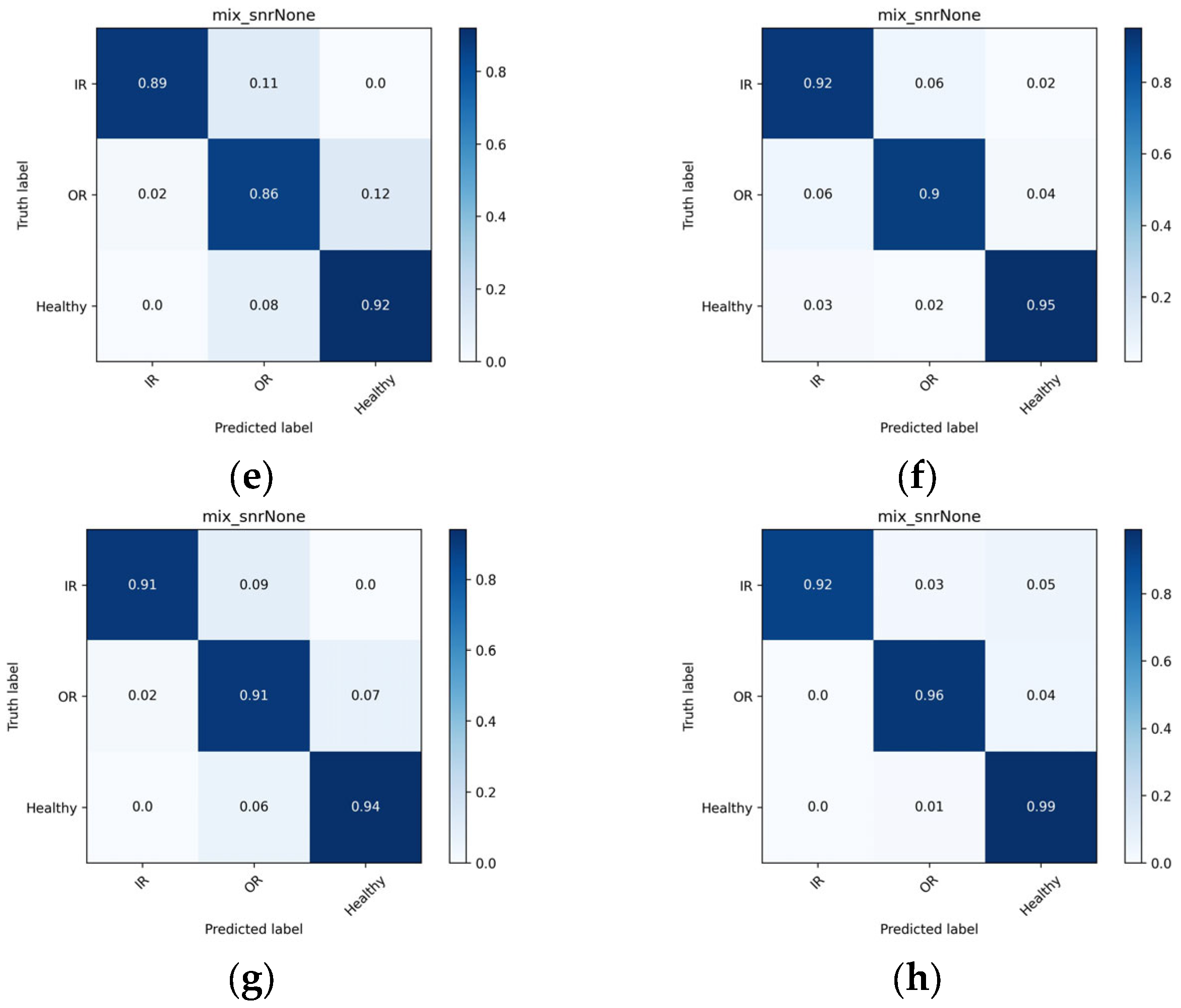
4.5.2. Confusion Matrix Analysis

To further confirm the diagnostic impact of the approach described in this research, the confusion matrix was utilized to assess each model’s identification capacity for various rolling bearing failure states, as shown in Figure 13. The other networks show significant variances in fault recognition accuracy for different states of rolling bearings. The ShuffleNetV2 and ResNet50 networks have lower diagnosis rates for outer ring faults, and further observation reveals that these networks mainly misclassify outer-ring faults as healthy states, which indicates that these models did not sufficiently extract the feature information of the outer-ring faults, whereas the method used in this paper, by incorporating the CCA and focusing on the key channel information in the feature map, enhanced the model. The method proposed in this paper also had a better bearing fault diagnosis capability in the PU dataset, as demonstrated by the accuracy of the model in this paper, which was higher than 92% for the fault diagnosis of the three states of rolling bearings and up to 99% for recognizing the normal state of rolling bearings.

5. Conclusions

A rolling bearing fault detection approach based on the improved residual network model was suggested to solve the issues of inadequate feature extraction and excessive model complexity, which resulted in high computational costs in existing fault diagnostic methods. The CCA mechanism is integrated into the residual block to improve feature representation, which allowed the network to learn richer and more discriminative features. Depth-separable convolution replaces ordinary convolution in the residual block, which significantly reduced the number of model parameters and amount of computation. The Meta-Acon activation function enhanced the model’s capacity to adapt and generalize. The model’s performance was validated by the CWRU and PU datasets, with fault classification accuracies of 99.95% and 95.7%, respectively. It outperformed ShuffleNetV2, MobileNetV2, VGG16, ResNet18, ResNet50, Swin-T, and ECA_ResNet. The model required only 0.53 MB and 0.49 GF of parameters and achieved a high fault recognition accuracy under a variable load and noise. The approach presented in this study was characterized by high accuracy, modest computational and parametric quantities, and good generalization, and may be utilized to diagnose rolling bearing faults.

References

1. Liu, J.; Hu, Y.; Wang, Y.; Wu, B.; Fan, J.; Hu, Z. An integrated multi-sensor fusion-based deep feature learning approach for rotating machinery diagnosis. Meas. Sci. Technol. 2018, 29, 055103. [Google Scholar] [CrossRef]
2. Wu, G.; Yan, T.; Yang, G.; Chai, H.; Cao, C. A review on rolling bearing fault signal detection methods based on different sensors. Sensors 2022, 22, 8330. [Google Scholar] [CrossRef]
3. Zhang, X.; Zhao, B.; Lin, Y. Machine learning based bearing fault diagnosis using the case western reserve university data: A review. IEEE Access 2021, 9, 155598–155608. [Google Scholar] [CrossRef]
4. Zhu, Z.; Lei, Y.; Qi, G.; Chai, Y.; Mazur, N.; An, Y.; Huang, X. A review of the application of deep learning in intelligent fault diagnosis of rotating machinery. Measurement 2023, 206, 112346. [Google Scholar] [CrossRef]
5. Hakim, M.; Omran, A.A.B.; Ahmed, A.N.; Al-Waily, M.; Abdellatif, A. A systematic review of rolling bearing fault diagnoses based on deep learning and transfer learning: Taxonomy, overview, application, open challenges, weaknesses and recommendations. Ain Shams Eng. J. 2023, 14, 101945. [Google Scholar] [CrossRef]
6. Yang, H.; Li, X.; Zhang, W. Interpretability of deep convolutional neural networks on rolling bearing fault diagnosis. Meas. Sci. Technol. 2022, 33, 055005. [Google Scholar] [CrossRef]
7. Janssens, O.; Slavkovikj, V.; Vervisch, B.; Stockman, K.; Loccufier, M.; Verstockt, S.; Van de Walle, R.; Van Hoecke, S. Convolutional neural network based fault detection for rotating machinery. J. Sound Vib. 2016, 377, 331–345. [Google Scholar] [CrossRef]
8. Fu, W.; Jiang, X.; Li, B.; Tan, C.; Chen, B.; Chen, X. Rolling bearing fault diagnosis based on 2D time-frequency images and data augmentation technique. Meas. Sci. Technol. 2023, 34, 045005. [Google Scholar] [CrossRef]
9. Wang, H.; Du, W. Multi-source information deep fusion for rolling bearing fault diagnosis based on deep residual convolution neural network. Proc. Inst. Mech. Eng. Part C J. Mech. Eng. Sci. 2022, 236, 7576–7589. [Google Scholar] [CrossRef]
10. Neupane, D.; Kim, Y.; Seok, J. Bearing fault detection using scalogram and switchable normalization-based CNN (SN-CNN). IEEE Access 2021, 9, 88151–88166. [Google Scholar] [CrossRef]
11. Irfan, M.; Mushtaq, Z.; Khan, N.A.; Mursal, S.N.F.; Rahman, S.; Magzoub, M.A.; Latif, M.A.; Althobiani, F.; Khan, I.; Abbas, G. A Scalo gram-based CNN ensemble method with density-aware smote oversampling for improving bearing fault diagnosis. IEEE Access 2023, 11, 127783–127799. [Google Scholar] [CrossRef]
12. Hao, X.; Zheng, Y.; Lu, L.; Pan, H. Research on intelligent fault diagnosis of rolling bearing based on improved deep residual network. Appl. Sci. 2021, 11, 10889. [Google Scholar] [CrossRef]
13. Song, X.; Cong, Y.; Song, Y.; Chen, Y.; Liang, P. A bearing fault diagnosis model based on CNN with wide convolution kernels. J. Ambient Intell. Humaniz. Comput. 2022, 13, 4041–4056. [Google Scholar] [CrossRef]
14. Plakias, S.; Boutalis, Y.S. Fault detection and identification of rolling element bearings with Attentive Dense CNN. Neurocomputing 2020, 405, 208–217. [Google Scholar] [CrossRef]
15. Wang, P.; Chen, J. Fault diagnosis of spent fuel shearing machines based on improved residual network. Ann. Nucl. Energy 2024, 196, 110228. [Google Scholar]
16. Chen, Y.; Zhan, W.; Jiang, Y.; Zhu, D.; Guo, R.; Xu, X. DDGAN: Dense Residual Module and Dual-stream Attention-Guided Generative Adversarial Network for colorizing near-infrared images. Infrared Phys. Technol. 2023, 133, 104822. [Google Scholar] [CrossRef]
17. Wang, Y.; Zou, Y.; Hu, W.; Chen, J.; Xiao, Z. Intelligent fault diagnosis of hydroelectric units based on radar maps and improved GoogleNet by depthwise separate convolution. Meas. Sci. Technol. 2023, 35, 025103. [Google Scholar] [CrossRef]
18. Saghi, T.; Bustan, D.; Aphale, S.S. Bearing fault diagnosis based on multi-scale CNN and bidirectional GRU. Vibration 2022, 6, 11–28. [Google Scholar] [CrossRef]
19. Yu, X.; Wang, Y.; Liang, Z.; Shao, H.; Yu, K.; Yu, W. An adaptive domain adaptation method for rolling bearings’ fault diagnosis fusing deep convolution and self-attention networks. IEEE Trans. Instrum. Meas. 2023, 72, 1–14. [Google Scholar] [CrossRef]
20. Karnavas, Y.L.; Plakias, S.; Chasiotis, I.D. Extracting spatially global and local attentive features for rolling bearing fault diagnosis in electrical machines using attention stream networks. IET Electr. Power Appl. 2021, 15, 903–915. [Google Scholar] [CrossRef]
21. Ren, H.; Liu, S.; Wei, F.; Qiu, B.; Zhao, D. A novel two-stream multi-head self-attention convolutional neural network for bearing fault diagnosis. Proc. Inst. Mech. Eng. Part C J. Mech. Eng. Sci. 2024, 238, 5393–5405. [Google Scholar] [CrossRef]
22. Gou, L.; Li, H.; Zheng, H.; Li, H.; Pei, X. Aeroengine control system sensor fault diagnosis based on CWT and CNN. Math. Probl. Eng. 2020, 2020, 5357146. [Google Scholar] [CrossRef]
23. Yan, R.; Shang, Z.; Xu, H.; Wen, J.; Zhao, Z.; Chen, X.; Gao, R.X. Wavelet transform for rotary machine fault diagnosis: 10 years revisited. Mech. Syst. Signal Process. 2023, 200, 110545. [Google Scholar] [CrossRef]
24. He, K.; Zhang, X.; Ren, S.; Sun, J. Deep residual learning for image recognition. In Proceedings of the 2016 IEEE Conference on Computer Vision and Pattern Recognition, Las Vegas, NV, USA, 27–30 June 2016. [Google Scholar]
25. Zhou, Y.; Kang, X.; Ren, F.; Lu, H.; Nakagawa, S.; Shan, X. A multi-attention and depthwise separable convolution network for medical image segmentation. Neurocomputing 2024, 564, 126970. [Google Scholar] [CrossRef]
26. Huang, Z.; Wang, X.; Huang, L.; Huang, C.; Wei, Y.; Liu, W. CCNet: Criss-Cross Attention for Semantic Segmentation. In Proceedings of the IEEE/CVF International Conference on Computer Vision (ICCV 2019), Seoul, Republic of Korea, 27 October–2 November 2019; pp. 603–612. [Google Scholar]
27. Ma, N.; Zhang, X.; Liu, M.; Sun, J. Activate or not: Learning customized activation. In Proceedings of the IEEE/CVF Conference on Computer Vision and Pattern Recognition, Nashville, TN, USA, 20–25 June 2021. [Google Scholar]
28. Wei, X.; Zhang, X.; Li, Y. SARN: A lightweight stacked attention residual network for low-light image enhancement. In Proceedings of the 2021 6th International Conference on Robotics and Automation Engineering (ICRAE), Guangzhou, China, 19–22 November 2021. [Google Scholar]
29. Case Western Reserve University Bearing Data Center Website. Available online: https://eecs.cwru.edu (accessed on 20 June 2024).
30. Lessmeier, C.; Kimotho, J.K.; Zimmer, D.; Sextro, W. Condition monitoring of bearing damage in electromechanical drive systems by using motor current signals of electric motors: A benchmark data set for data-driven classification. In Proceedings of the PHM Society European Conference, Bilbao, Spain, 5–8 July 2016. [Google Scholar]
31. Liu, Z.; Lin, Y.; Cao, Y.; Hu, H.; Wei, Y.; Zhang, Z.; Lin, S.; Guo, B. Swin transformer: Hierarchical vision transformer using shifted windows. In Proceedings of the IEEE/CVF International Conference on Computer Vision, Montreal, BC, Canada, 11–17 October 2021. [Google Scholar]
32. Sandler, M.; Howard, A.; Zhu, M.; Zhmoginov, A.; Chen, L.C. Mobilenetv2: Inverted residuals and linear bottlenecks. In Proceedings of the IEEE Conference on Computer Vision and Pattern Recognition, Salt Lake City, UT, USA, 18–23 June 2018. [Google Scholar]
33. Zhang, X.; Zhou, X.; Lin, M.; Sun, J. Shufflenet: An extremely efficient convolutional neural network for mobile devices. In Proceedings of the IEEE Conference on Computer Vision and Pattern Recognition, Salt Lake City, UT, USA, 18–23 June 2018. [Google Scholar]
34. Yang, X.; Sun, S.; Wang, G.; Shi, N.; Xie, Y. Bearing fault diagnosis method based on ECA_ResNet. Bearing 2023. (published online in Chinese). Available online: http://kns.cnki.net/kcms/detail/41.1148.th.20230414.1947.004.html (accessed on 20 June 2024).
35. Van der Maaten, L.; Hinton, G. Visualizing data using t-SNE. J. Mach. Learn. Res. 2008, 9, 2579–2605. [Google Scholar]
Figure 1. ResNet residual block.
Electronics 13 03749 g001
Figure 2. Ordinary convolution process.
Electronics 13 03749 g002
Figure 3. Deeply separable convolutional processes.
Electronics 13 03749 g003
Figure 4. CCA network structure.
Electronics 13 03749 g004
Figure 5. Structure of residual block.
Electronics 13 03749 g005
Figure 6. Improved residual network model.
Electronics 13 03749 g006
Figure 7. The diagnostic process of improved residual network.
Electronics 13 03749 g007
Figure 8. Bearing condition monitoring test bench, University of Paderborn, Germany.
Electronics 13 03749 g008
Figure 9. Time–frequency images of each state of bearings: (a) normal; (b) outer-ring failure; (c) inner-ring fault; (d) rolling body failure.
Electronics 13 03749 g009
Figure 10. Comparison of fault identification effects of different models under variable load environments.
Electronics 13 03749 g010
Figure 11. Visualization of the output of each network module: (a) classification results of convolutional initialization; (b) after the first residual block; (c) after the second residual block; (d) the output of softmax.
Electronics 13 03749 g011aElectronics 13 03749 g011b
Figure 12. The confusion matrix under noiselessness.
Electronics 13 03749 g012
Figure 13. Confusion matrices: (a) Shuffle NetV2; (b) MobileNet V2; (c) VGG16; (d) ResNet18; (e) ResNet50; (f) Swin-T; (g) ECA_ResNet; (h) our model.
Electronics 13 03749 g013aElectronics 13 03749 g013b