Article

Fault Diagnosis of Wind Turbine Component Based on an Improved Dung Beetle Optimization Algorithm to Optimize Support Vector Machine

1
Hebei Provincial Key Laboratory of Information Fusion and Intelligent Control, Shijiazhuang 050024, China
2
College of Engineering, Hebei Normal University, Shijiazhuang 050024, China
*
Author to whom correspondence should be addressed.
Electronics 2024, 13(18), 3621; https://doi.org/10.3390/electronics13183621
Submission received: 27 July 2024 / Revised: 8 September 2024 / Accepted: 9 September 2024 / Published: 12 September 2024

Abstract

:
Due to high probability of blade faults, bearing faults, sensor faults, and communication faults in pitch systems during the long-term operation of wind turbine components, and the complex operation environment which increases the uncertainty of fault types, this paper proposes a fault diagnosis method for wind turbine components based on an Improved Dung Beetle Optimization (IDBO) algorithm to optimize Support Vector Machine (SVM). Firstly, the Halton sequence is initially employed to populate the population, effectively mitigating the issue of local optima. Secondly, the subtraction averaging optimization strategy is introduced to accelerate the dung beetle algorithm in solving complex problems and improve its global optimization ability. Finally, incorporating smooth development variation helps improve data quality and the accuracy of the model. The experimental results indicate that the IDBO-optimized SVM (IDBO-SVM) achieves a 96.7% fault diagnosis rate for wind turbine components. With the proposed IDBO-SVM method, fault diagnosis of wind turbine components is more accurate and stable, and its practical application is excellent.

1. Introduction

To combat global climate change, achieve low-carbon development, protect the ecological environment, and meet “carbon peaking and carbon neutrality” goals, the vigorous development of clean energy has become a universal trend. Wind turbines are also developing toward larger unit capacities [1]. Wind turbines operate in an environment with strong uncertainty and resistance. On the one hand, the wind speed and direction in wind farms are changeable and difficult to determine. On the other hand, the main equipment works in the open sky at high altitude and is subject to the combined effects of direct sunlight, rain splashing and sand erosion in adverse weather for a long time, which brings certain difficulties to the operation of the unit [2]. As an important component of the control system for wind turbine generators, the pitch system can make the wind turbine maintain high-efficient operation under various wind speed conditions and achieve maximum wind energy conversion efficiency by regulating the angle of the blades [3]. Figure 1 shows the pitch system for a wind turbine. Meanwhile, by mitigating the impact of extreme wind conditions on the wind turbine, it can also prevent damage to the wind turbine, thus greatly ensuring the safety and reliability of wind power generation [4].
The main components of the variable pitch system of a wind turbine include a speed controller, a power controller, a pitch controller, and a generator [5]. Figure 2 shows the control system of the variable pitch system in a wind turbine.
As seen in Figure 2, the pitch system has a complex structure and contains many types of components. During system operation, it is prone to blade faults, bearing faults, sensor faults, and communication faults. Different faults have various impacts on the whole system. For instance, blade failure can result in damage or failure of the blades, bearing failure can cause instability or damage to rotating components, sensor failure can lead to decreased data accuracy, and communication failure can result in delays in transmitting fault information. Therefore, it is very important to classify faults in order to improve the reliability of wind turbine generators. By classifying faults, different types of faults can be better understood and identified. This enables targeted preventive and maintenance measures to be implemented, the system will therefore operate more efficiently.
Regarding the fault problems of the pitch system in wind turbine generators, Shigang Q. [6] proposed a wind turbine fault diagnosis method based on a multi-channel attention mechanism. Iker E [7] employed sensor data algorithms to diagnose pitch system faults. Kandukuri T S [8] introduced a sensor-based fault diagnosis approach for wind turbines. Li Hongchuan [9] based on fault tree theory, a fault diagnosis method was proposed. He classified various causes of pitch system faults and unit shutdowns and established a fault tree analysis model. Yin Zikang [10] compared AT-LSTM with RNN and LSTM and developed an AT-LSTM model for predicting pitch health status. The above experts’ research on wind turbine fault diagnosis has played a promoting role, but its inadequacy lies in the low diagnostic accuracy. The success of SVM in generalization has been improved by introducing optimization algorithms in recent years. Support Vector Machines (SVM), robust machine learning algorithms, are extensively used in medical diagnosis, industrial control, and financial prediction [11].
SVM, as a supervised learning method, has performed exceptionally well in classification and regression problems. It also has powerful non-linear classification capabilities. Using its high-dimensional mapping capabilities, it can find the most optimal hyperplane in complex fault feature scenarios. Ling Lu [12] optimized support vector machine with Dung Beetle Optimizer algorithm (DBO) for transformer fault identification and improved the fault identification rate. Other commonly used algorithms include the Football Team Training Algorithm (FTTA) [13], Zebra Optimization Algorithm (ZOA) [14], Gray Wolf Optimization algorithm (GWO) [15], Snake Optimization algorithm (SO) [16], Artificial Rabbit Optimization algorithm (ARO) [17], etc. Despite the improvements in performance, the speed is still too slow. This work tackles the issues of low prediction accuracy and slow convergence in traditional fault diagnosis methods within high-dimensional data environments by offering the following contributions:
(1)
This paper summarizes the background and research status of wind turbine fault diagnosis and points out the value of support vector machine algorithms in fault diagnosis. The common fault forms of wind turbine are introduced.
(2)
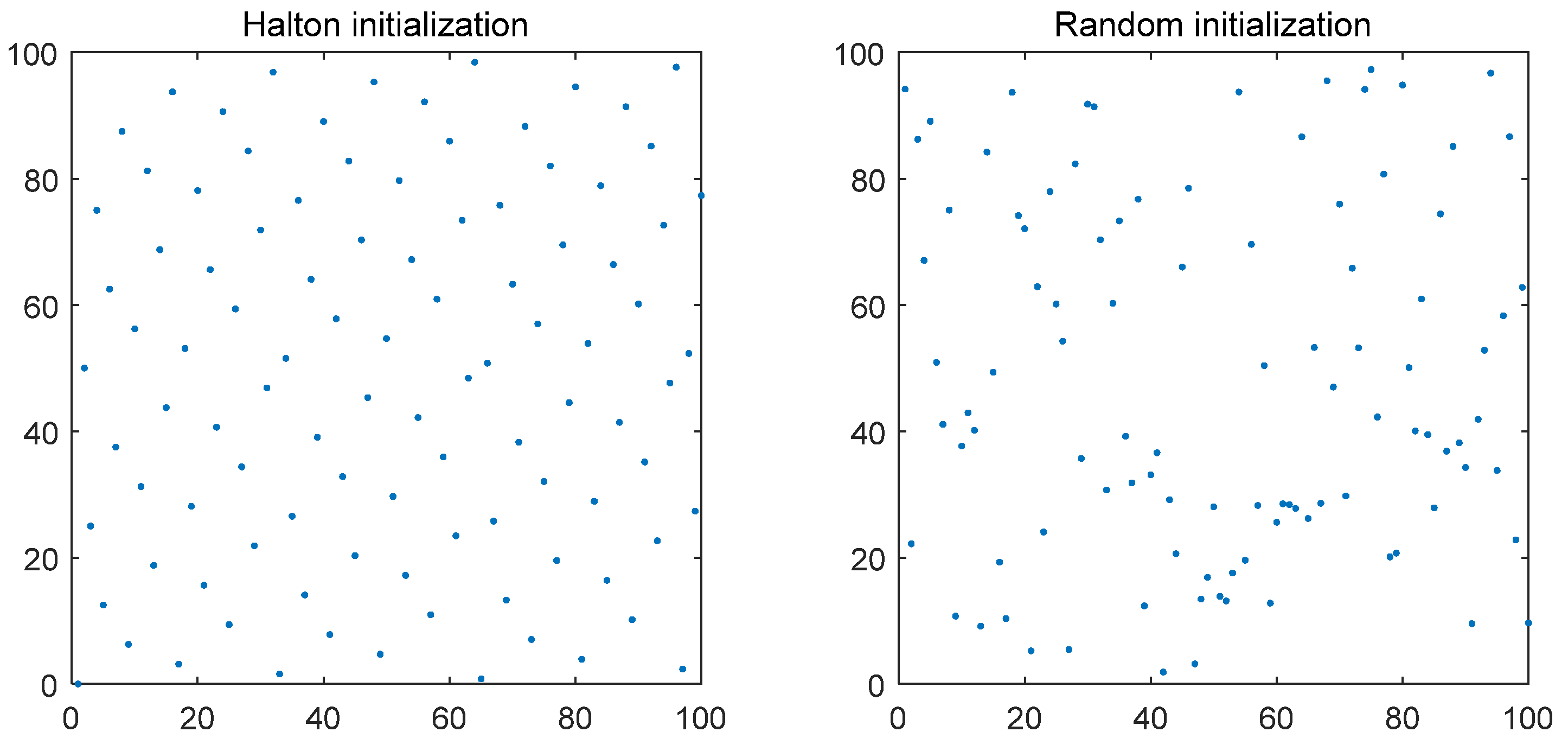
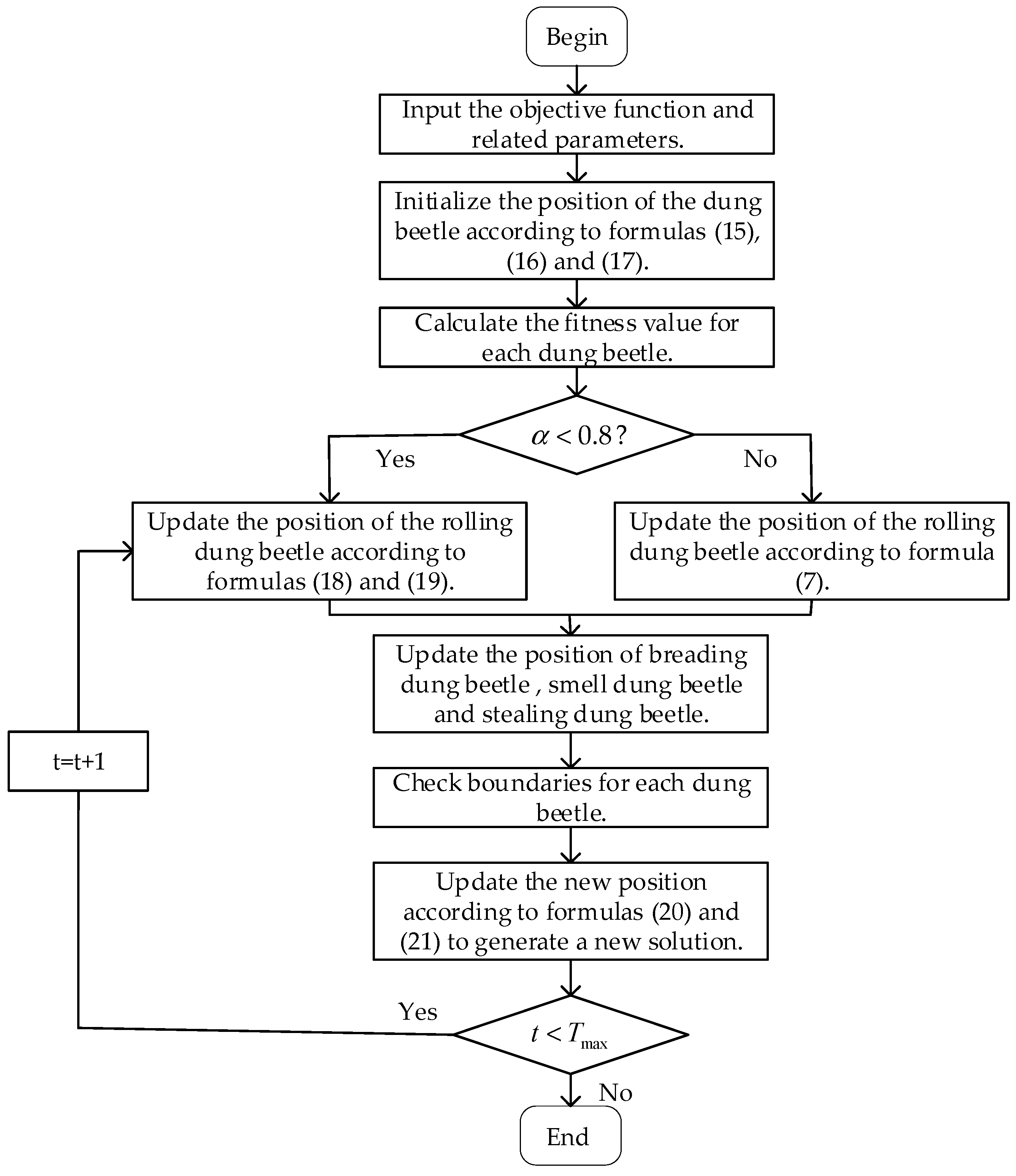
Halton sequence initialization, subtraction average optimization strategy, and smooth development variation were added to improve the DBO algorithm—which solved the problems of uneven population distribution and easily fall into the local optimal solution—and proposed an IDBO-SVM fault diagnosis model.
(3)
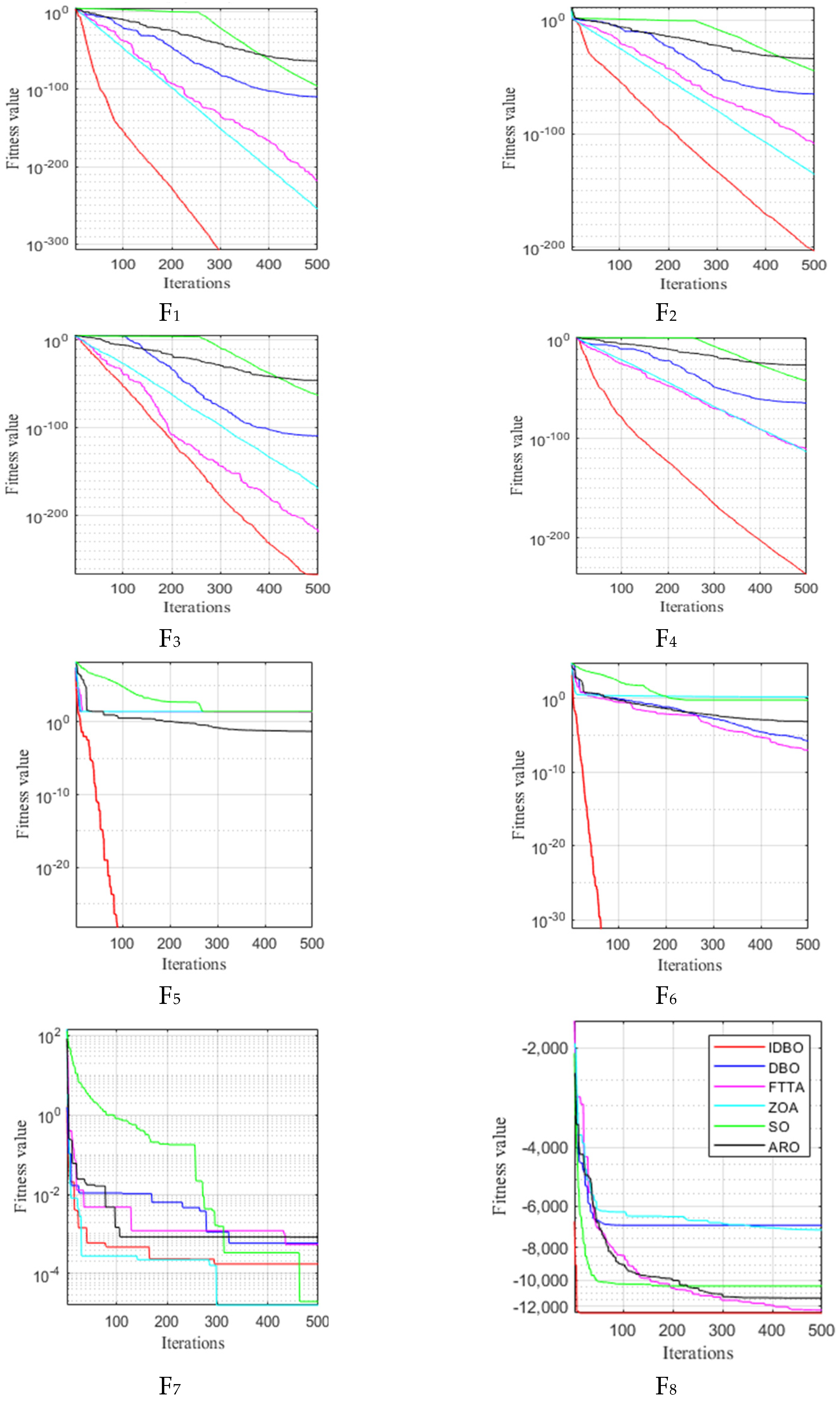
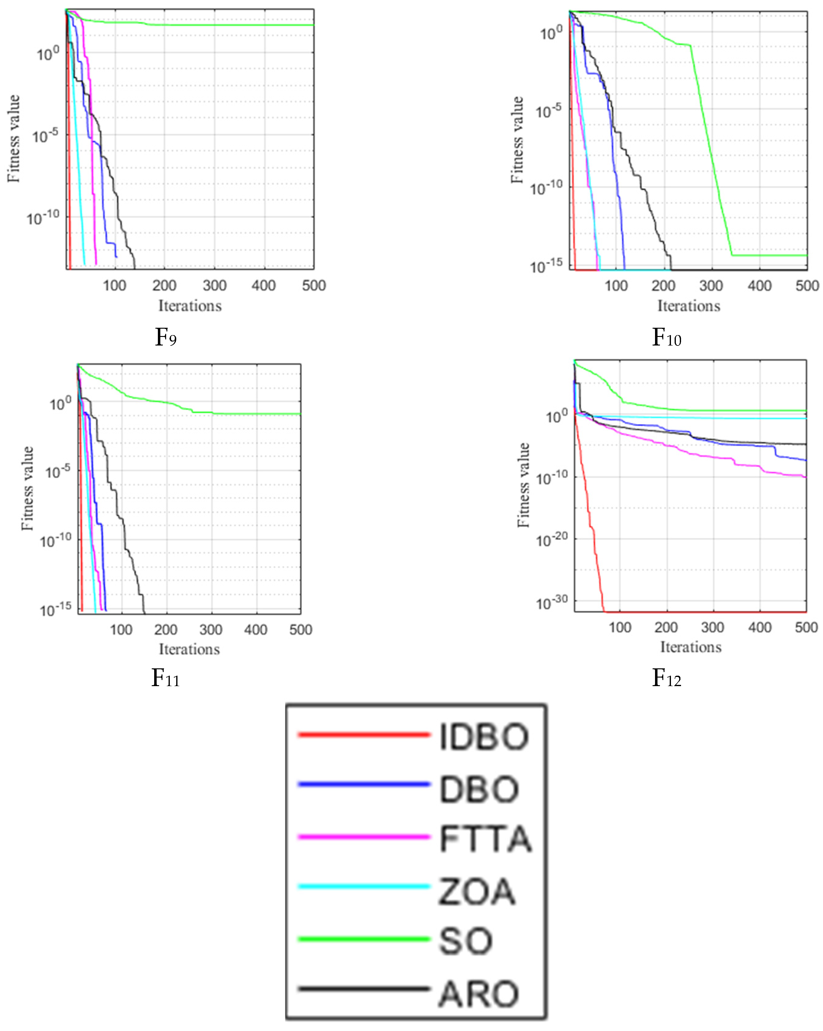
The convergence and performance of IDBO algorithm on 12 standard test functions are evaluated and compared with the DBO algorithm, FTTA, ZOA, SO algorithm, and ARO algorithm.
(4)
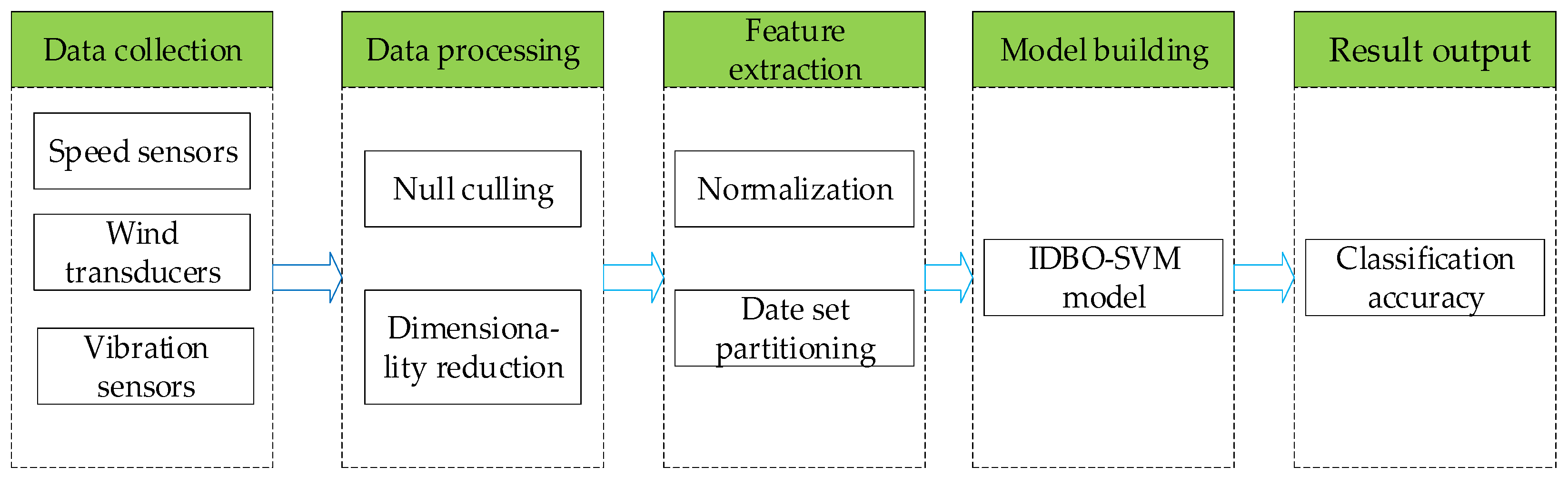
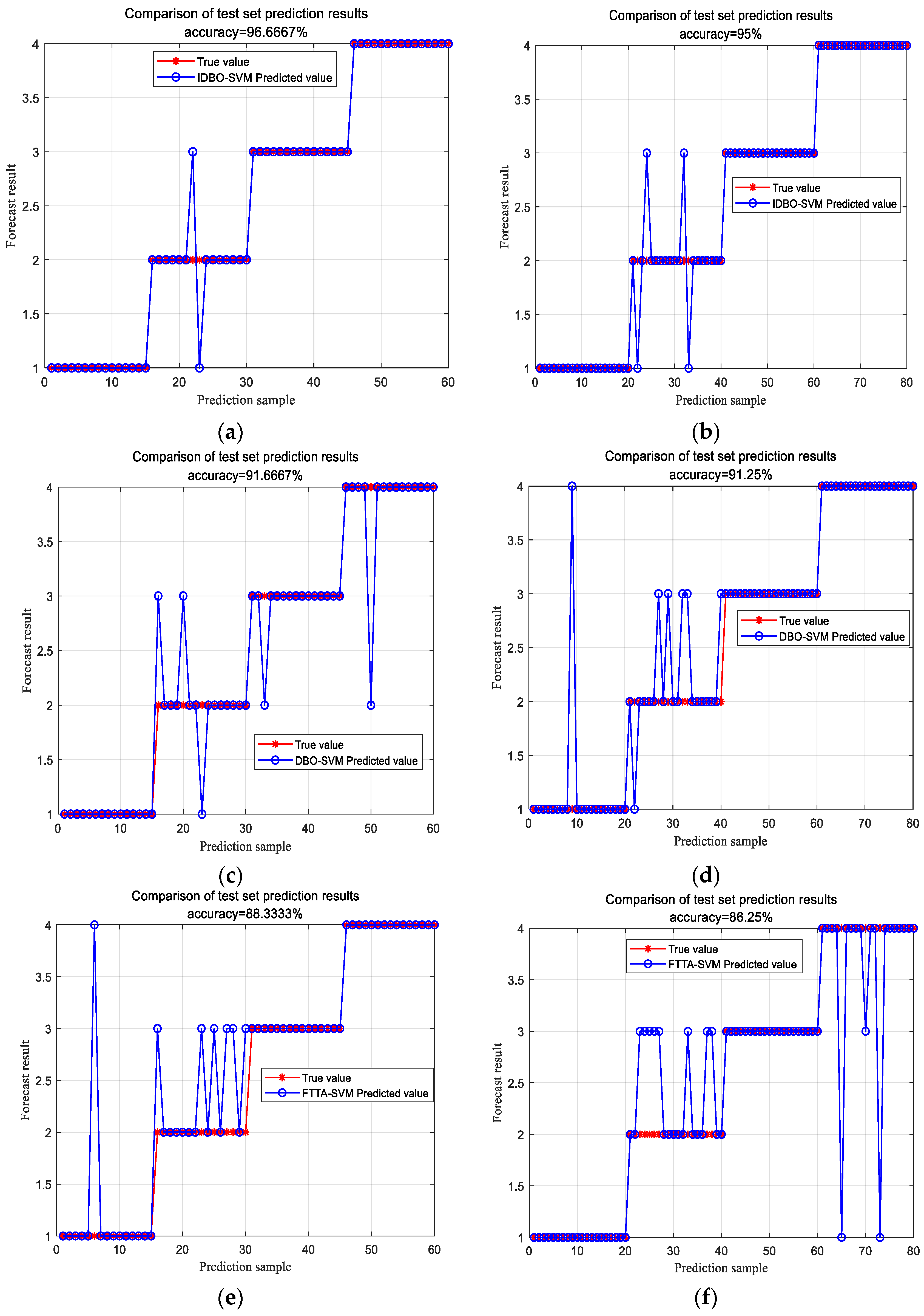
Two sets of data of wind turbine under normal environment and severe environment are collected by using speed sensors, wind transducers, and vibration sensors. Each set of data includes six parameters: wind speed, wind direction, rotor speed, rotor position, power and pitch angle. The experimental results show that the average fault diagnosis rate reaches about 96% under the two conditions, which improves the reliability and stability of the wind power system.
The structure of this article is as follows: Section 1 describes common faults of variable pitch systems in wind turbines and some scholars’ contributions in fault diagnosis. Section 2 briefly reviews the SVM and DBO algorithms. In Section 3, we improve the algorithm. Section 4 presents corresponding test experiments. Finally, Section 5 summarizes the paper the full text and the future research direction.

2. Basic Principle

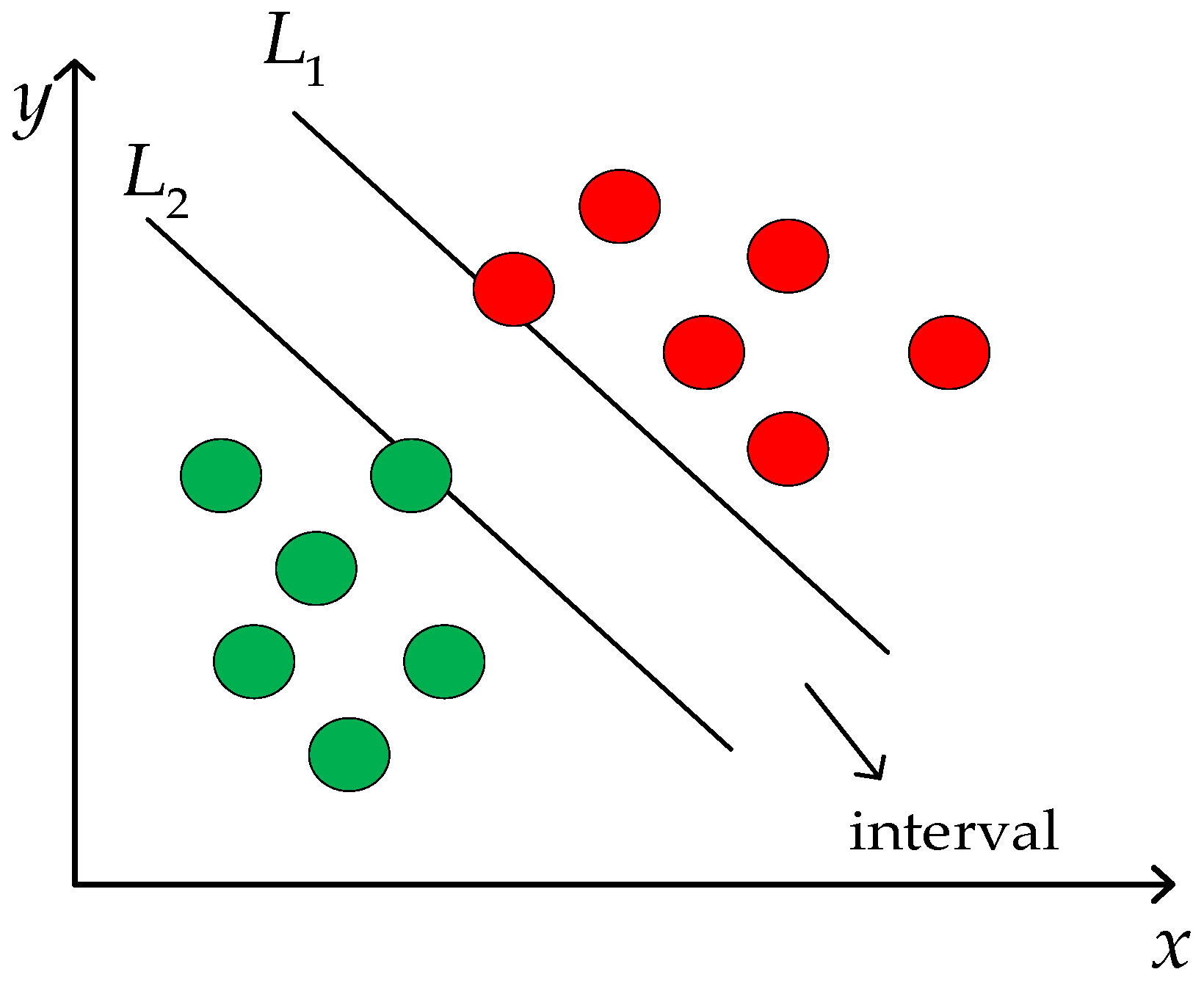
2.1. Support Vector Machines

Support vector machine is a kind of supervised classifier, which has the advantages of learning high-dimensional data and practical ability [18]. After training, SVM can obtain an optimal hyperplane and two classification boundaries. All sample points within the two classification boundaries are called positive samples, and others are called negative samples. If a sample point is exactly on the classification boundary, it belongs to both positive and negative classes. Taking two-dimensional data as an example, the classification is shown in Figure 3.
In the figure above, green circles and red circles represent data from two different categories. Lines L 1 and L 2 are the upper and lower optimal classification lines. The expression of the hyperplane is denoted as:
f ( X ) = ω T X + b
The optimization objective of support vector machine can be written as:
min J ( ω , ξ ) = 1 2 | | ω | | 2 + C i = 1 N ξ i , s . t . y i f ( X i ) 1 ξ i , i = 1 , 2 , , N .
In the formula: ξ i is a relaxation variable used to control training error and maintain constraints. C parameter balances the trade-off between model complexity and empirical risk.
However, in reality, non-linear data is often encountered. To achieve linearity in the sample data, it is necessary to map the low-dimensional non-linear data to a high-dimensional space. By introducing the kernel function, the inner product of high-dimensional vectors ϕ ( x ) and ϕ ( y ) in feature space after dimension lifting can be calculated using low-dimensional vectors x and y in the input sample space. The definition of the kernel function is:
k ( x , y ) = ϕ ( x ) T ϕ ( y )
This paper provides analysis of three aspects: nonlinearity, number of parameters, and parameter sensitivity. It selects the radial basis kernel function, which is suitable for nonlinear problems; has fewer parameters; and has high parameter sensitivity as the kernel function used in this paper. Its expression is:
K ( x , x i ) = e x x i 2 2 g 2
In the formula, g is the parameter of the kernel function.
The kernel function g and penalty factor c are the two most important parameters in SVM. Setting appropriate values of g and c can effectively improve the accuracy of support vector machine classification [19].

2.2. Dung Beetle Optimization Algorithm

The Dung Beetle Optimization algorithm (DBO) is inspired by the habits of the dung beetle. It utilizes swarm intelligence principles to simulate how dung beetles interact with each other and roll dung balls [20]. Numerous optimization issues, including parameter tuning and function optimization, have been addressed using the DBO method. It has strong generalization. Compared with some optimization algorithms, parameter setting in DBO is relatively simple and does not require a large amount of parameter tuning.

2.2.1. Ball Rolling Dung Beetles

There is a fascinating habit among dung beetles in which they form dung balls and then roll them to the ideal position. For the dung ball to roll straight, the dung beetle relies on celestial cues [21]. The dung beetles update their position as they roll the ball. Rolling mathematical models are represented as follows:
x i ( t + 1 ) = x i ( t ) + α × k × x i ( t 1 ) + b × Δ x
Δ x = | x i ( t ) X w |
where t presents the current iteration number, x i ( t ) represents the position information of the i dung beetle in the t iteration, k ( 0 , 0.2 ] , α is a natural coefficient assigned a value of −1 or 1, X ω represents the global worst position and simulates light intensity changes.
Dung beetles need to dance when they encounter obstacles that prevent them from moving forward. Therefore, the dung beetle’s dancing behavior can be described as follows:
x i ( t + 1 ) = x i ( t ) + tan ( θ ) | x i ( t ) x i ( t 1 ) |
where θ [ 0 , π ] , if θ = 0, θ = π / 2 or θ = π , the position of the dung beetle will not be updated.

2.2.2. Breeding Dung Beetles

A dung beetle hides the dung balls in a safe place in nature. Selecting a suitable spawning site is crucial for dung beetles to ensure a safe environment for their offspring [22]. Inspired by the above discussion, in order to replicate the female dung beetle spawning habitat, the following boundary selection technique is suggested:
L b = max ( X × ( 1 R ) , L b )
U b = min ( X × ( 1 R ) , U b )
where X * represents the current local best position; L b * and U b * represent the lower and upper bounds of the spawning area respectively, where R = ( 1 t ) / T max ; while L b and U b represent the optimization problem’s lower and upper bounds.
The DBO algorithm produces one egg for each iteration for each female dung beetle. This results in the breeding balls’ position changing during iteration, as shown below:
B i ( t + 1 ) = X + b 1 × ( B i ( t ) L b ) + b 2 × ( B i ( t ) U b )
where B i ( t ) represents the position information of the i breeding ball in the t iteration; b 1 and b 2 represent two independent random vectors of size 1 × D . Please note that the positions of breeding balls are strictly constrained within a certain range, namely the spawning area.

2.2.3. Small Dung Beetles

Some adult dung beetles, referred to as small dung beetles, emerge from the ground to search for food. Additionally, identifying the optimal foraging area is essential to simulate the natural foraging process of dung beetles. The optimal foraging area boundaries are defined as follows:
L b b = max ( X b × ( 1 R ) , L b )
U b b = min ( X b × ( 1 R ) , U b )
Consequently, the position update for the small dung beetles is as follows:
x i ( t + 1 ) = x i ( t ) + C 1 × ( x i ( t ) L b b ) + C 2 × ( x i ( t ) U b b )
where C 1 represents normally distributed random numbers, and C 2 is a random vector in the range (0, 1).

2.2.4. Stealing Dung Beetles

Among dung beetles, thieves steal dung balls from one another. Moreover, it can be seen from Formulas (11) and (12) that X b is the best food source. Therefore, we can assume that the area around X b is the best location for competing for food. The position data of the thieving beetles is updated during the iterative process, which can be explained as follows:
x i ( t + 1 ) = X b + S × g × ( | x i ( t ) X | + | x i ( t ) X b | )
where g is a random vector of size 1 × D subject to normal distribution and S represents a constant.

3. Improved Dung Beetle Optimization Algorithm

In view of dung beetle optimization’s problems of easy fall into local optimal, slow convergence speed, and sensitivity to initial solutions. The Halton sequence is employed during population initialization to effectively prevent the population from converging to a local optimum. In the dung-rolling stage, the subtraction average optimization strategy is introduced to accelerate the solution process of the beetle algorithm for complex problems. Finally, incorporating smooth development mutation helps improve data quality and enhance diagnostic accuracy.

3.1. Halton Sequence Initializes the Population

Population initialization is an indispensable stage for swarm intelligence optimization algorithms. Traditional population initialization methods rely on pseudo-random number generation. This method is easy to implement and has strong randomness [23], but the individuals in the population may not be uniformly distributed in the search space, thus missing a considerable part of the population space. The method of generating the initial population based on chaos technology is also widely used. Some studies have shown that using chaotic sequences for population initialization can achieve better results than pseudo-random numbers, but this method is globally stable and locally unstable and is highly sensitive to initial conditions and parameter settings [24]. Therefore, this paper introduces the more advanced sequence method, namely the Halton sequence, to initialize the population in order to increase population diversity.
Assume the search space is two-dimensional. Halton sequence implementation consists of the following steps: two prime numbers are selected as bases, corresponding to the two dimensions respectively. Each dimension is recursively subdivided and sampled according to the base within (0, 1), forming some non-repetitive and uniformly distributed points. The subdivision process is shown in the mathematical model of Formulas (15)–(17):
n = i = 0 m 0 a i p 1 i = a 0 + a 1 p 1 1 + + a m 0 p 1 m 0
ϕ p 1 ( n ) = a 0 p 1 1 + a 1 p 1 2 + + a m 0 p 1 m 0 1
H ( n ) = [ ϕ p 1 , 1 ( n ) , ϕ p 1 , 2 ( n ) ]
In the equation, n represents the ordinal number of the Halton sequence, p 1 represents the radix of the Halton sequence, α i { 0 , 1 , 2 , , p i 1 } is a constant variable, Φ p 1 ( n ) is a defined sequence function, and H ( n ) represents a two-dimensional uniform Halton sequence.
In a two-dimensional space, assuming a population size of 100 and upper and lower boundaries of 1 and 0, respectively, a comparison of the spatial distribution of individuals in the population is shown in Figure 4 for random distribution and Halton sequence distribution. The bases of the Halton sequences are base1 = 2 and base2 = 3.
As shown in Figure 4, the points in the random distribution graph are more dispersed, denser in some areas, and sparser in other areas. While the graph of Halton sequence distribution shows that the points are uniformly distributed throughout the entire space, with almost no obvious clustering or vacuum phenomena.
The population initialization using the Halton sequence can effectively avoid the situations of over-concentration or sparseness during population initialization, thereby improving the search efficiency and global search ability of the algorithm. This uniform distribution characteristic enables the algorithm to more comprehensively explore different regions in the solution space and reduces the risk of getting stuck in local optimal solutions. In the research of wind turbine fault diagnosis, this means that researchers can find the optimal solution or the best model parameters more quickly and accurately, thus significantly improving the efficiency and reliability of fault diagnosis.

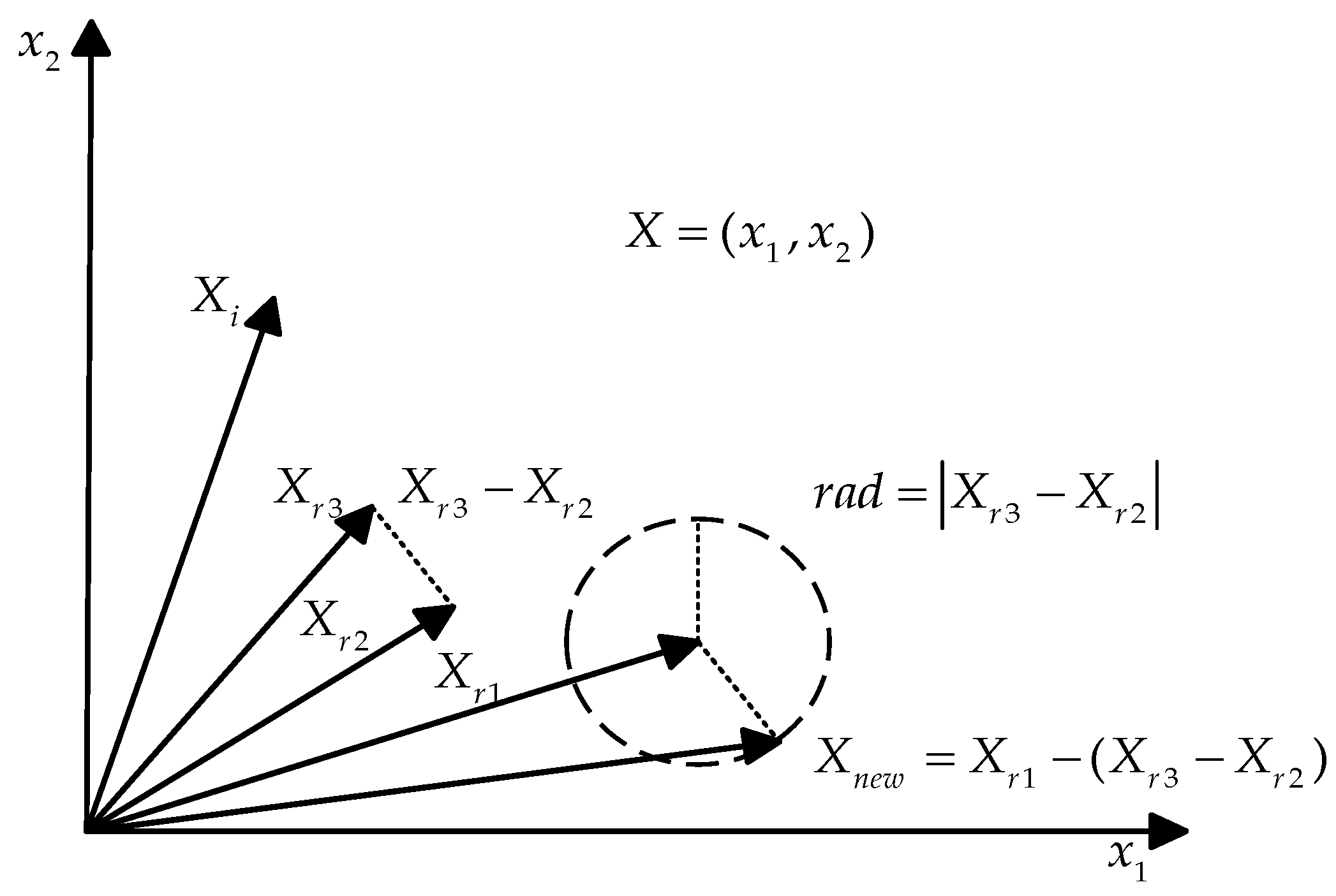
3.2. Subtraction Average Optimization Strategy

The Subtraction Average Optimization (SABO) algorithm is a mathematics-based optimization method. The search space encompasses the solution space for all optimization problems [25]. The dimension of the problem is defined by the number of choice variables, representing a subset of the search space [26]. A population of search agents makes up an algorithm. As a result, the search agent with the best objective function is computed.
Mathematical concepts such as averages, differences in search agent positions, and sign differences between objective function values inspire the design of SABO. In the proposed SABO, the displacement of a search agent X i is calculated by averaging v subtractions from each agent X j . Consequently, Equation (18) determines the new position of each search agent.
X i n e w = X i + r i 1 N j = 1 N ( X i v   X j )
where X i n e w is the newly updated position of the i search agent. Where N is the total number of search agents, and r 1 is an m-dimensional vector whose components take values from a normal distribution in the range [0, 1].
As long as the new position increases the objective function value, it is acceptable for the agent to hold it as its new position.
X i = { X i n e w , F i n e w < F i ; X i , e l s e ;
where F i and F i n e w are the objective function values of search agents X i and X i n e w respectively.
The subtraction averaging optimization strategy can effectively reduce the risk of over-fitting on the training set for the model. By introducing subtractive averaging during the model training process, it can reduce the model’s over-reliance on training samples and improve the model’s generalization ability for unseen samples. However, sometimes, this strategy can reduce the performance of the model, such as when introducing subtraction averaging without properly adjusting relevant parameters (such as the number or weight of search agents). This may lead to insufficient exploration ability during the search process, thereby limiting the performance of the model. This requires parameter tuning. Multiple experiments need to be conducted under different numbers of search agents and test the performance of the improved DBO algorithm, recording the results of each experiment, and finally selecting the parameters that can provide the best performance.

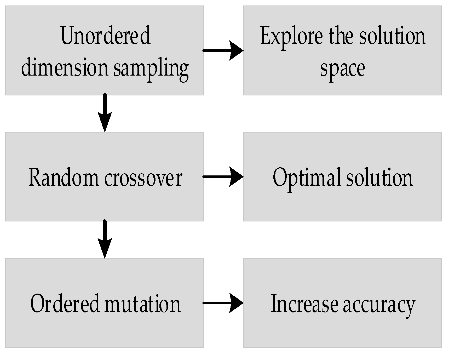
3.3. Smooth Development Variation

The smooth development variation contains unordered dimension sampling, random crossover and ordered mutation. Algorithm performance can be improved by combining these three mechanisms. As shown in Figure 5, the relationship between the three mechanisms and their impact on the algorithm.
Unordered dimension sampling is a preparatory step for the mutation process, providing new directions for subsequent mutation and crossover to make the solution exploration more random and diverse. Random crossover, on the basis of unordered dimensions, can more effectively combine existing solutions and generate new solutions through crossover. The new individuals generated through unordered dimension sampling and random crossover are finally fine-tuned through ordered mutation to achieve more precise searching.
The core of unordered dimension sampling lies in its ability to effectively help algorithms explore the solution space. Random crossover combines information from different individuals to produce new solutions and maintain population diversity. Ordered mutation refers to the ability to make fine-tuned adjustments to parameters in the algorithm, thus improving the accuracy of fault identification.

3.3.1. Unordered Dimension Sampling

In the search and development process, dimension selection is an important method for adjusting and optimizing search agents, aiming to achieve efficient information transmission. One dimension of evolutionary selection aligns with the most exploitative mechanism. In contrast, evolutionary search agents exhibit the highest level of exploratory mechanisms across all dimensions. Using the sampling theory as a reference, this study adopts the concept of dimension selection as a sampling method. In the case of an n-dimensional array, the sampling rate determines how many dimensions are involved. In that case, the dimensions that are involved are randomly sampled based on the sampling rate, while the dimensions that aren’t involved remain static. Unordered dimension sampling reduces the number of dimensions approaching the optimal agent, thereby preventing a decrease in overall sparsity.
Furthermore, unordered dimension sampling is beneficial for vectorization programming and reduces system running time.
The sampling rate is calculated by Formula (20):
R a t e s a m p l e = c e i l ( max ( t max I t e r , ε 1 ) × dim )
where R a t e s a m p l e is the sampling rate, c e i l ( ) rounds the number up, ε 1 is the minimum number of participants to avoid both the early lower sampling rates and the non-linear characteristic of the sampling rate.

3.3.2. Random Crossover

The dimensions selected through unordered dimension sampling can be combined with random crossover to fully explore this search space, wherein random crossover improves diversity and expands the search range by randomly selecting individuals as the starting point for exploration. The radius of exploration is determined by the distance between two other random individuals. As a result, running the search agent can escape local optima and learn population distribution information. With an increasing radius, the running agent perceives the entire population as being in the exploration phase. When the radius decreases, it can be assumed that the entire population is in the exploitation phase.
As shown in Figure 6, in a two-dimensional search space, three individuals— X r 1 , X r 2 , and X r 3 —are randomly selected to generate a new position vector X n e w , while the previous position vector X i escapes from the local optimum. It is worth noting that the direction of the difference between X r 2 and X r 3 is kept unchanged in order to increase the range of the exploration space. The absolute difference between dimensions X r 2 and X r 3 forces uniform movement, reducing population diversity and hindering search agent evolution.
Random crossover is represented as:
X t ( t + 1 ) = X r 1 ( X r 3 X r 2 ) r 1 , r 2 , r 3 i
where r 1 , r 2 , r 3 is a randomly selected index.

3.3.3. Ordered Mutation

Ordered mutation is an exploratory approach for dimensions chosen by sampling unordered ones. By implementing ordered mutation, new solutions that differ from the current solution in certain dimensions can be generated, helping the algorithm to escape from local optima. The combination of ordered mutation and random crossover enhances search efficiency. Ordered mutation uses the arithmetic mean as shown in Formula (22):
X i ( t + 1 ) = ( X i ( t ) + X i 1 ( t ) ) 2
where X i ( t ) is the i individual, X i 1 ( t ) is the previous individual, and X i ( t + 1 ) is the new position vector. When the exponent i is equal to 1, the previous one is the last individual in the population.
Smoothing developing variation handling data can make data smoother and more continuous, which helps to improve the model’s ability to capture fault features and diagnose accuracy. In practical applications, the operational data of wind turbines are often affected by various factors, including environmental changes, equipment aging, and operational conditions, which may cause noise and abnormal fluctuations in the data. By smoothing these variant data, the interference of noise can be effectively reduced, making the data show clearer trends and patterns.

3.3.4. IDBO-SVM Fault Diagnosis Model

In wind turbine pitch system fault diagnosis, traditional DBO-SVM models struggle with complex and diverse fault conditions, particularly in escaping local optimal solutions. This paper introduces an IDBO-SVM model to improve performance and suitability for diagnosing faults in wind turbine pitch systems.
Firstly, this paper adds Halton sequence initialization of the population in the initialization stage of the DBO algorithm. Using the Halton sequence to initialize the population can ensure a uniform distribution of sample points, fully cover the feature space, avoid overlap and aggregation between data samples. It solves the problem of non-uniform population distribution caused by traditional initialization.
Secondly, the IDBO-SVM model also introduces a subtraction averaging optimization strategy. The DBO algorithm uses a simple updating strategy in the process of finding solutions, resulting in low optimization efficiency. The introduction of subtractive averaging optimization strategy can promote the model’s overall learning of data features, rather than overfocusing on some specific samples or features. This can make the model better capture the overall distribution and regulation of data and improve efficiency.
Finally, incorporating smoothing development variation helps improve data quality and makes data clearer and more reliable. When faced with multivariate complex data, it can eliminate peaks and fluctuations in the data, making the data more continuous and consistent. This is conducive to the model more accurately learning the patterns and rules of the data, improving the model’s predictive ability and accuracy. Specifically, the steps are:
Step 1: Normalize the wind turbine datasets.
Step 2: Initialize the population using Halton sequences.
Step 3: Introduce subtraction averaging optimization strategy to update the position of each individual in the population.
Step 4: Update the positions of the breeding ball, minions, and thieves.
Step 5: Perform boundary judgment for each firefly.
Step 6: Process each individual and introduce smoothing development variation to update the new position and generate new solutions.
Step 7: Repeat the previous steps until the global optimal solution satisfies the termination criteria, then output the fitness value.
Set the maximum iteration number of the population to T max , the population size to N, and the threshold to 0.8.
The workflow of the algorithm is shown in Figure 7:
The core of the proposed IDBO-SVM algorithm is to utilize the global search ability and classification performance of the IDBO algorithm to complete accurate fault classification. In this method, the whole process includes 5 key steps: data collection, data processing, feature extraction, model building and result output. The detailed process of wind turbine fault diagnosis based on IDBO-SVM is shown in Figure 8.

4. Discussion

Two aspects are examined in this paper to validate the effectiveness of the proposed method. First, the IDBO algorithm is evaluated broadly using 12 standard test functions.
The Wilcoxon rank sum test method is adopted to test the convergence and speed of the IDBO algorithm in different functions. Second, the same wind farm and wind turbine type data are selected to further validate the effectiveness of the IDBO algorithm in fault diagnosis of wind turbine systems when using actual wind farm data.

4.1. Comparison of Convergence and Performance between IDBO and Other Algorithms

4.1.1. Introduction of Test Functions

To test the optimization performance of the IDBO algorithm, this paper selects 12 standard test functions from the benchmark test functions to perform optimization testing on the IDBO algorithm, including F1–F7 as single-peak test functions and F8–F12 as multi-peak test functions. The selected benchmark functions contain different features such as different local extremes and different complexities. By using functions with different features, we can examine the algorithm’s ability to handle complexity and nonlinear relationships, ensuring the algorithm has wide applicability. Each benchmark function has its specific variable value range. The setting of the variable range is to ensure that the algorithm optimizes within a reasonable and effective search space. Different functions may show completely different performances within different value ranges. Table 1 presents the 12 standard test functions.

4.1.2. Convergence Analysis of IDBO and Other Algorithms

To validate the convergence of the IDBO algorithm, this paper selects Dung Beetle Optimizer (DBO), Football Team Training Algorithm (FTTA), Zebra Optimization Algorithm (ZOA), Snake Optimizer (SO), and Artificial Rabbits Optimization (ARO) for comparison. To ensure the comparability of experimental results, the population size N = 40 and maximum number of iterations Max = 500 were uniformly set for experiments of each algorithm. Convergence analysis of each algorithm was conducted using the 12 benchmark test functions in Table 1, and the results are compared as shown in Figure 9.
As can be seen from Figure 9, for functions F1, F2, F3, and F4, the convergence accuracy of FTTA, ZOA, SO, ARO, and DBO are all relatively low. DBO has higher convergence accuracy on functions F5, F7, and F8 but converges too slowly, while the IDBO algorithm rapidly converges from the beginning of iterations and finds the theoretical optimal value. For function F1, the IDBO algorithm rapidly converges from the beginning of iterations with significantly higher convergence accuracy. The convergence curves of the function prove that IDBO has a faster convergence speed when optimizing standard test functions, thereby demonstrating the effectiveness of IDBO.

4.1.3. Performance Comparison between IDBO and Other Algorithms

To fully validate the performance of the algorithms, statistical analysis is conducted on the results of the proposed IDBO algorithm and the compared algorithms to determine whether IDBO is significantly better than other algorithms from a statistical perspective. In order to determine whether two algorithms are significantly different, Wilcoxon rank sum analysis is used. In this test, an indicator called p-value is used to determine the significant difference. The Wilcoxon rank sum test is performed at the 5% significance level, and the 5% significance level has become a standard norm in many fields, including medicine, psychology, engineering, and computer science. The selection of the 5% significance level increases the credibility of the evaluation results. Significant results obtained at this level mean that we are more confident in the performance evaluation of the improved algorithm, reducing misjudgments caused by randomness or external factors. Too low significance levels (such as 1%) may require more sample quantities, while too-high significance levels may make the judgment not rigorous enough. When p < 5%, it indicates that there is a significant difference between the two compared algorithms. Otherwise, it indicates that the difference in optimization performance between the two algorithms is not significant.
This study evaluates five algorithms by independently solving each one 12 times, with a population size of N = 40 and 500 iterations, across 12 standard test functions. The aim is to identify significant differences between the results of the IDBO algorithm and those of the five comparison algorithms. The P values results of the Wilcoxon statistical test are shown in Table 2.
Table 2 shows that most p-values are below 5%, demonstrating the statistically significant superiority of the proposed IDBO algorithm compared to the other five algorithms. Comprehensive analysis of solution accuracy, convergence curves of test functions, and Wilcoxon rank sum test results indicates that the IDBO algorithm significantly enhances both local and global capabilities. It outperforms the DBO, FTTA, ZOA, SO, and ARO algorithms in terms of convergence speed, accuracy, and stability.

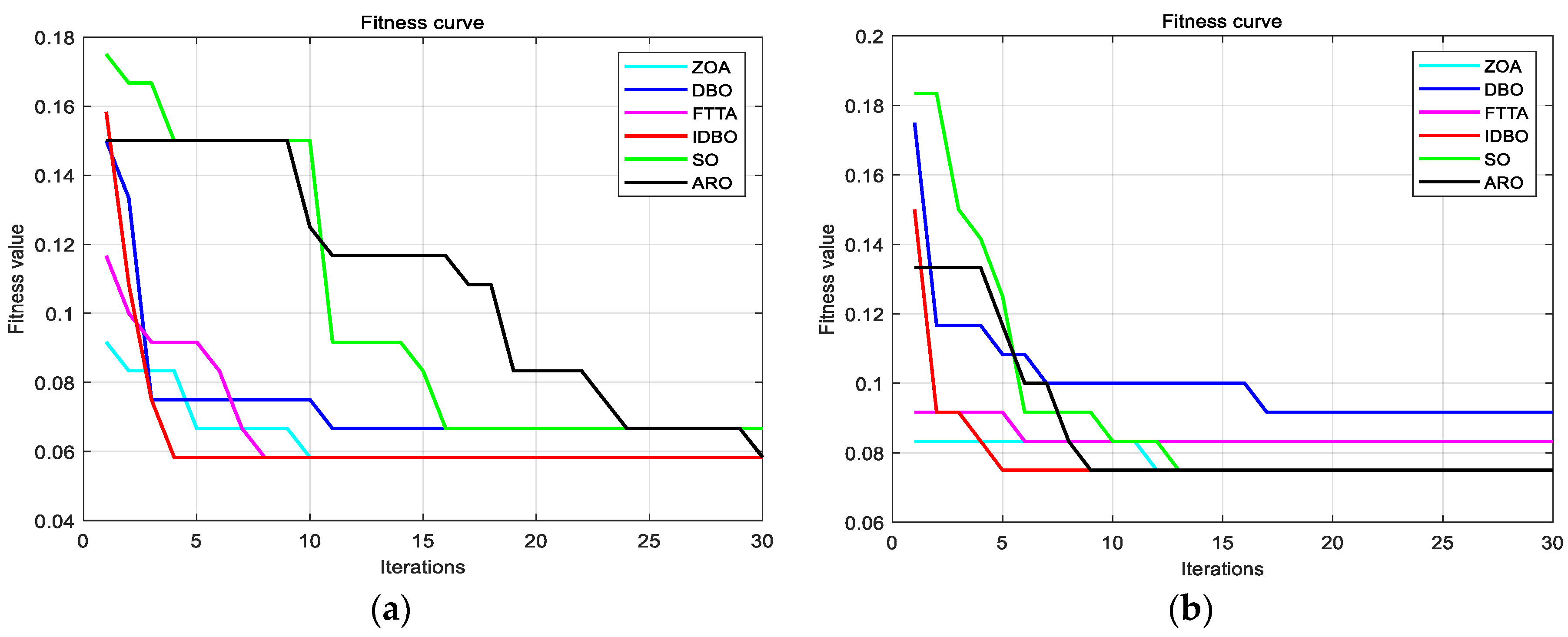
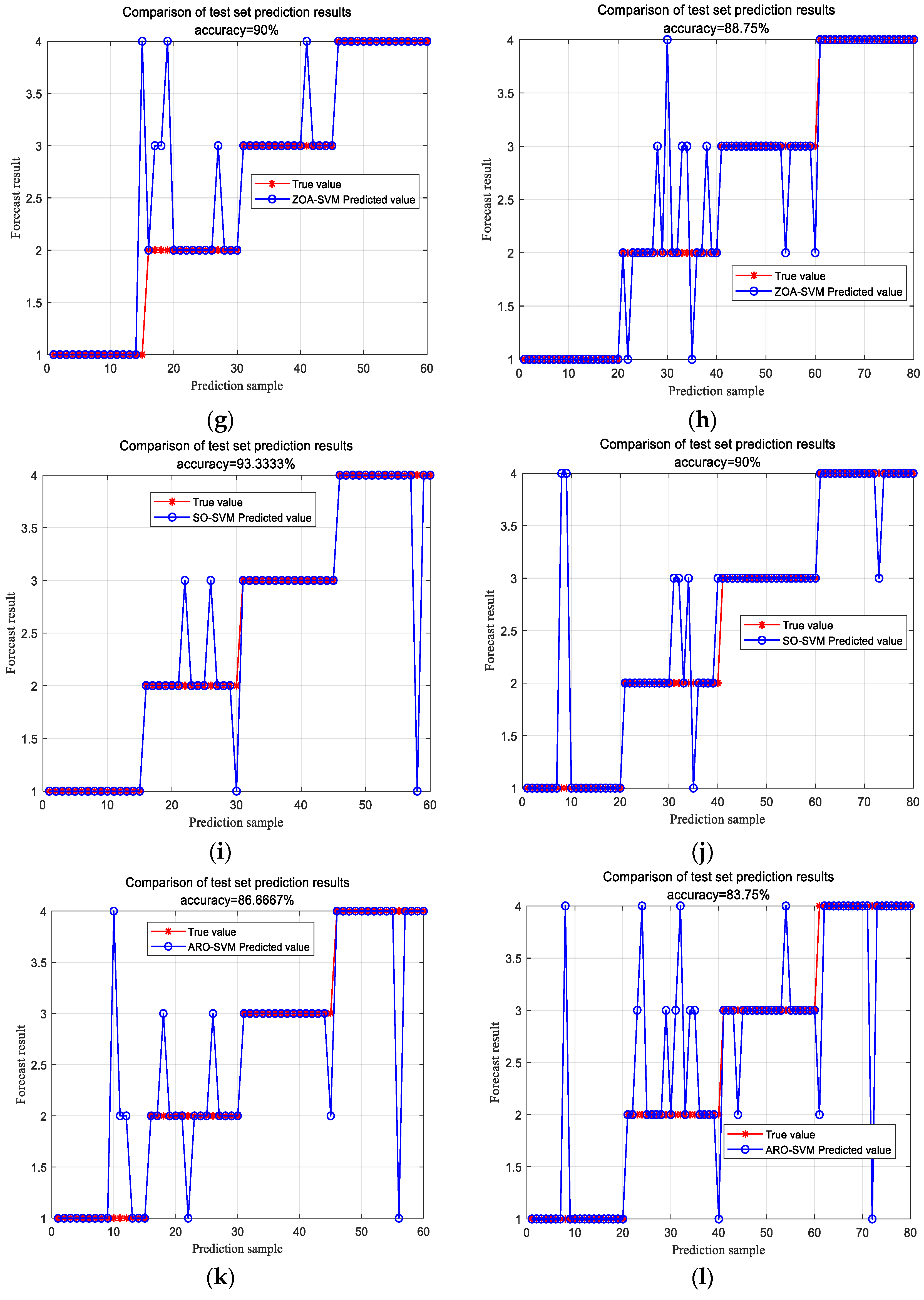
4.2. Case Study Analysis

This paper uses data from the same type of wind turbine unit collected at a wind farm in Baoding City, Hebei Province, China under two working scenarios in April 2020. One is data under normal environmental conditions (appropriate temperature and humidity), and the other is data under severe environmental conditions (strong winds and relatively low temperature). The instrument parameters used in the experiment are shown in Table 3.
The data parameters collected in the experiment are shown in Table 4.
Sensors such as speed sensors, wind transducers and vibration sensors were used to collect data from different faulty units every 30 min. Through principal component analysis of the proportion of each characteristic value, empty value data, shutdown data, and characteristics with lower proportions were removed. Ultimately, the data were divided into 200 samples, each with 6 dimensional attributes. The fault categories were divided into four types: blade fault, bearing fault, sensor fault, and communication fault.
In order to demonstrate that the IDBO algorithm has a faster convergence speed and higher diagnostic accuracy, the random permutation function randperm is used to randomly shuffle the collected data set, thereby eliminating potential order bias. Firstly, we selected 60% of the datasets as the training set for model training, with the remaining 40% as the test set for evaluating the model’s generalization ability. This ratio is based on extensive experiments and theoretical analysis, with the aim of balancing the adequacy of model training and independence of testing. Secondly, the divided data will be normalized to avoid the imbalance influence on model training caused by features with large values. Finally, model training and experimental testing are carried out using IDBO-SVM.
As shown in Figure 10, the iterative curve graphs of each optimization algorithm under the two environments are set with 30 iterations.
The fitness value in the fitness curve changes with the increase in the number of iterations, which can reflect the convergence speed of the algorithm. If the fitness value rapidly decreases and tends to be stable during the iteration process, it indicates that the algorithm has a faster convergence speed. Figure 10 demonstrates that the IDBO algorithm exhibits a significantly higher iteration speed compared to the other five optimization algorithms in both environments. This enhances the search efficiency and accelerates the identification of the optimal solution, thereby optimizing the wind turbine fault diagnosis process using support vector machines.
The classification simulation results of each optimization algorithm under the two environments are shown in Figure 11.
The evaluation indexes of the diagnostic results of each optimization algorithm under the two environments are shown in Table 5.
As can be seen from Table 5, the improved DBO optimization algorithm and the original DBO optimization algorithm have increased the fault diagnosis rate by an average of 4.5% under the two environments. Compared with the other four optimization algorithms, the fault diagnosis rate has been increased by an average of 7.5%. The enhanced DBO optimization SVM—incorporating Halton distribution initialization, subtraction average optimization strategy, and smooth development variation—increases the likelihood of finding the global optimal solution and enhances both performance and iteration speed. These advantages collectively enhance the model’s accuracy in diagnosing faults in complex variable pitch systems, thereby improving the reliability and stability of wind power systems.

5. Conclusions

For the fault diagnosis problem of the variable pitch system in wind turbine units, a new DBO optimization support vector machine algorithm is proposed. The original DBO algorithm has introduced Halton sequence initialization in the initialization stage, which avoids clustering of data samples and helps improve the model’s generalization ability and accuracy. In the rolling ball beetle stage, the subtraction average optimization strategy was introduced, which enables the model to better capture the overall distribution of the data and make accurate diagnoses even when facing new, unseen data. The finally incorporated smoothing development variation makes the data more continuous and consistent, improving the predictive ability and accuracy of the model. The simulation experiments demonstrate that the optimized support vector machine model achieved good results. These results lead to two conclusions:
(1)
Twelve standard test functions were used to test the performance of IDBO. The experimental results showed that the IDBO algorithm has a faster convergence rate than the other five optimization algorithms.
(2)
Apply the six optimization algorithms to the identical wind farm and unit model. Compared to the other five algorithms, the IDBO algorithm has higher diagnostic accuracy, improving the diagnosis accuracy rate to 96.67%. The limitations of this study are the data collection is on a small number of specific wind farms, so the model performance may differ under different climate conditions, wind speed variations and load conditions. Therefore, future research will consider combining IDBO algorithm with deep learning methods to make full use of the feature extraction capability of deep neural networks, so that the model can better capture complex nonlinear relationships.

Author Contributions

Conceptualization, Q.L.; methodology, M.L.; software, C.F.; validation, J.W.; formal analysis, M.L.; investigation, J.W.; resources, C.F.; data administration, Q.L. and M.L.; writing—original draft preparation, Q.L.; writing—review and editing, M.L. and J.W.; supervision, J.W.; project administration, Q.L. All authors have read and agreed to the published version of the manuscript.

Funding

This work was supported by the doctoral research project of Hebei Normal University (No. L2022B25).

Data Availability Statement

Data sets generated during the current study are available from the corresponding author on reasonable request.

Conflicts of Interest

The authors declare no conflicts of interest.

Nomenclature

DBODung beetle optimization
SVMSupport vector machine
IDBOImproved dung beetle optimization
FTTAFootball team training algorithm
ZOAZebra optimization algorithm
SOSnake optimization
AROArtificial rabbit optimization
GWOGray wolf optimization
c Penalty factor
g Kernel parameter
t The number of iterations of the population
T max The maximum number of iterations in a population
dim The maximum dimension of a vector

References

  1. Liu, D.; Zhang, F.; Dai, J.; Xiao, X.; Wen, Z. Study of the Pitch Behaviour of Large-Scale Wind Turbines Based on Statistic Evaluation. IET Renew. Power Gener. 2021, 15, 2315–2324. [Google Scholar] [CrossRef]
  2. Huang, Z.; Liu, Q.; Hao, Y. Research on Temperature Distribution of Large Permanent Magnet Synchronous Direct Drive Wind Turbine. Electronics 2023, 12, 2251. [Google Scholar] [CrossRef]
  3. Lan, J.; Chen, N.; Li, H.; Wang, X. A review of fault diagnosis and prediction methods for wind turbine pitch systems. Int. J. Green Energy 2024, 21, 1613–1640. [Google Scholar] [CrossRef]
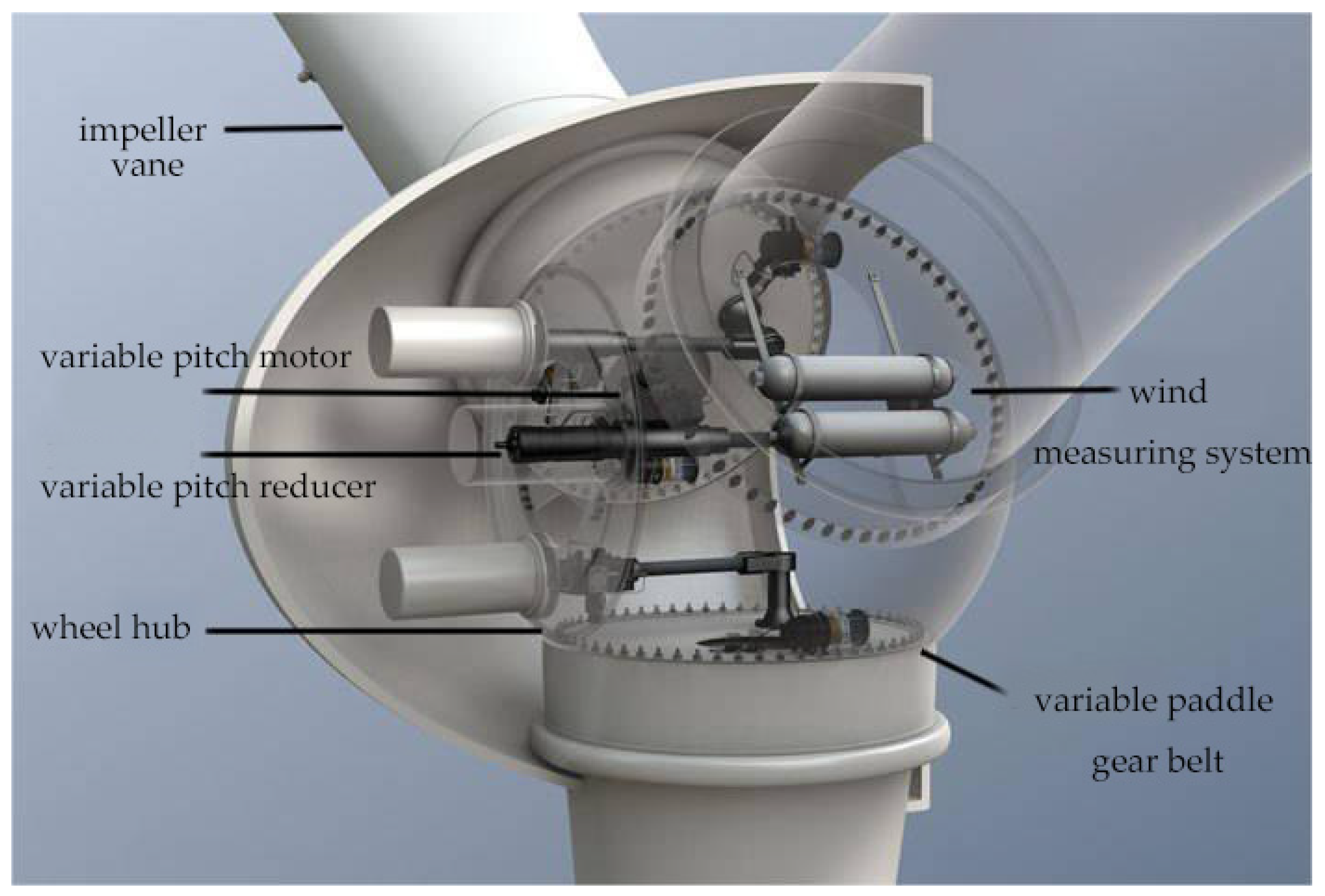
  4. Ding, G.; Liu, Y.; Guo, Y. Design of variable pitch system for large wind turbine unit. Wind Energy 2021, 7, 104–107. [Google Scholar]
  5. Song, R. Research on Fault Diagnosis Method of Variable Pitch System of Wind Turbine. Equip. Manag. Maint. 2024, 4, 25–28. [Google Scholar]
  6. Shigang, Q.; Jie, T.; Zhilei, Z. Fault diagnosis of wind turbine pitch system based on LSTM with multi-channel attention mechanism. Energy Rep. 2023, 10, 104087–104096. [Google Scholar]
  7. Elorza, I.; Arrizabalaga, I.; Zubizarreta, A.; Martín-Aguilar, H.; Pujana-Arrese, A.; Calleja, C. A Sensor Data Processing Algorithm for Wind Turbine Hydraulic Pitch System Diagnosis. Energies 2021, 15, 33. [Google Scholar] [CrossRef]
  8. Kandukuri, S.T.; Klausen, A.; Robbersmyr, K.G. Fault diagnostics of wind turbine electric pitch systems using sensor fusion approach. J. Phys. Conf. Ser. 2018, 1037, 032036. [Google Scholar] [CrossRef]
  9. Li, H.C.; Wang, X.D.; Wang, D.M.; Cao, C.Y.; Chen, N.C.; Pan, W.G. Research on fault diagnosis of wind turbine variable pitch system based on fault tree. Equip. Manag. Maint. 2022, 168–169. [Google Scholar]
  10. Yin, Z.K.; Lin, Z.W.; Lv, G.H.; Li, D.Z. Research on fault diagnosis and health status prediction of wind turbine variable pitch system based on data-driven. J. Northeast Electr. Power Univ. 2023, 43, 1–11+17. [Google Scholar]
  11. Jamadar, I.M.; Nithin, R.; Nagashree, S.; Prasad, V.P.; Preetham, M.; Samal, P.K.; Singh, S. Spur Gear Fault Detection Using Design of Experiments and Support Vector Machine (SVM) Algorithm. J. Fail. Anal. Prev. 2023, 23, 2014–2028. [Google Scholar] [CrossRef]
  12. Lu, L.; Zhang, X.; Ma, H.; Pu, Q.; Lu, Y.; Xu, H. Transformer fault acoustic identification model based on acoustic denoising and DBO-SVM. J. Electr. Eng. Technol. 2024, 19, 3621–3633. [Google Scholar] [CrossRef]
  13. Hou, J.; Cui, Y.; Rong, M. An Improved Football Team Training Algorithm for Global Optimization. Biomimetics 2024, 9, 419. [Google Scholar] [CrossRef] [PubMed]
  14. Trojovská, E.; Dehghani, M.; Trojovský, P. Zebra optimization algorithm: A new bio-inspired optimization algorithm for solving optimization problems. IEEE Access 2022, 10, 49445–49473. [Google Scholar] [CrossRef]
  15. Lan, P.; Xia, K.; Pan, Y.; Fan, S. An improved GWO algorithm optimized RVFL model for oil layer prediction. Electronics 2021, 10, 3178. [Google Scholar] [CrossRef]
  16. Hashim, F.A.; Hussien, A.G. Snake Optimizer: A novel meta-heuristic optimization algorithm. Knowl. Based Syst. 2022, 242, 108320. [Google Scholar] [CrossRef]
  17. Wang, R.; Zhang, S.; Jin, B. Improved multi-strategy artificial rabbits optimization for solving global optimization problems. Sci. Rep. 2024, 14, 18295. [Google Scholar] [CrossRef]
  18. Li, L.; Meng, W.; Liu, X.; Fei, J. Research on rolling bearing fault diagnosis based on variational modal decomposition parameter optimization and an improved support vector machine. Electronics 2023, 12, 1290. [Google Scholar] [CrossRef]
  19. Amaya-Tejera, N.; Gamarra, M.; Vélez, J.I.; Zurek, E. A distance-based kernel for classification via Support Vector Machines. Front. Artif. Intell. 2024, 7, 1287875. [Google Scholar] [CrossRef]
  20. Pan, J.; Li, S.; Zhou, P.; Yang, G.L.; Lv, D.C. An improved dung beetle colony optimization algorithm guided by sine algorithm. Comput. Eng. Appl. 2023, 59, 92–110. [Google Scholar]
  21. Zhang, D.; Zhang, C.; Han, X.; Wang, C. Improved DBO-VMD and optimized DBN-ELM based fault diagnosis for control valve. Meas. Sci. Technol. 2024, 35, 075103. [Google Scholar] [CrossRef]
  22. He, J.; Guo, W.; Wang, S.; Chen, H.; Guo, X.; Li, S. Application of Multi-Strategy Based Improved DBO Algorithm in Optimal Scheduling of Reservoir Groups. Water Resour. Manag. 2024, 38, 1883–1901. [Google Scholar] [CrossRef]
  23. Sun, L.; Xin, Y.; Chen, T.; Feng, B. Rolling Bearing Fault Feature Selection Method Based on a Clustering Hybrid Binary Cuckoo Search. Electronics 2023, 12, 459. [Google Scholar] [CrossRef]
  24. Zhang, G.F. Research on optimization of construction project management based on genetic algorithm. J. Xinyang Agric. For. Coll. 2020, 30, 126–129+133. [Google Scholar]
  25. Jiang, Y.; Ding, Y. A Target Localization Algorithm for a Single-Frequency Doppler Radar Based on an Improved Subtractive Average Optimizer. Remote Sens. 2024, 16, 2123. [Google Scholar] [CrossRef]
  26. Moustafa, G.; Tolba, M.A.; El-Rifaie, A.M.; Ginidi, A.; Shaheen, A.M.; Abid, S. A subtraction-average-based optimizer for solving engineering problems with applications on TCSC allocation in power systems. Biomimetics 2023, 8, 332. [Google Scholar] [CrossRef]
Figure 1. Wind turbine pitch system.
Electronics 13 03621 g001
Figure 2. Block diagram of the variable pitch system control of a wind turbine.
Electronics 13 03621 g002
Figure 3. Classification diagram.
Electronics 13 03621 g003
Figure 4. Initialize the population space with Halton distribution and random distribution.
Electronics 13 03621 g004
Figure 5. The relationship between the three mechanisms and their impact on the algorithm.
Electronics 13 03621 g005
Figure 6. Random crossover in a two-dimensional space.
Electronics 13 03621 g006
Figure 7. The workflow diagram of IDBO-SVM.
Electronics 13 03621 g007
Figure 8. Process flow chart of fault diagnosis based on IDBO-SVM.
Electronics 13 03621 g008
Figure 9. Convergence curves of some test functions.
Electronics 13 03621 g009aElectronics 13 03621 g009b
Figure 10. The iterative curve graphs of each optimization algorithm under the two environments: (a) The iterative curve graphs of each optimization algorithm under the normal environment. (b) The iterative curve graphs of each optimization algorithm under the severe environment.
Electronics 13 03621 g010
Figure 11. The classification simulation result graphs of each optimization algorithm under the two environments: (a) IDBO-SVM (normal). (b) IDBO-SVM (severe). (c) DBO-SVM (normal). (d) DBO-SVM (severe). (e) FTTA-SVM (normal). (f) FTTA-SVM (severe). (g) ZOA-SVM (normal). (h) ZOA-SVM (severe). (i) SO-SVM (normal). (j) SO-SVM (severe). (k) ARO-SVM (normal). (l) ARO-SVM (severe).
Electronics 13 03621 g011aElectronics 13 03621 g011b
Table 1. Standard test functions.
Serial NumberFunctionDimRangeMin
1 F 1 ( x ) = i = 1 n x i 2 30[–100, 100]0
2 F 2 ( x ) = i = 1 n | x i | + i = 1 n | x i | 30[–10, 10]0
3 F 3 ( x ) = i = 1 n ( j 1 i x j ) 2 30[–100, 100]0
4 F 4 ( x ) = max { | x i | , 1 i n } 30[–100, 100]0
5 F 5 ( x ) = i = 1 n [ 100 ( x i + 1 x i 2 ) 2 + ( x i 1 ) 2 ] 30[–30, 30]0
6 F 6 ( x ) = i = 1 n ( [ x i + 0.5 ] ) 2 30[–100, 100]0
7 F 7 ( x ) = i = 1 n i x i 4 + r a n d o m [ 0 , 1 ) 30[−1.28, 1.28]0
8 F 8 ( x ) = i = 1 n x i sin ( | x i | ) 30[–500, 500]−418.98
9 F 9 ( x ) = i = 1 n [ x i 2 10 cos ( 2 π x i ) + 10 ] 30[−5.12, 5.12]0
10 F 10 ( x ) = 20 exp ( 0.2 1 n i = 1 n x i 2 ) exp ( 1 n i = 1 n cos ( 2 π x i ) ) + 20 + e 30[–32, 32]0
11 F 11 ( x ) = 1 4000 i = 1 n x i 2 i = 1 n cos ( x i i ) + 1 30[–600, 600]0
12 F 12 ( x ) = 0.1 { sin 2 ( 3 π x 1 ) + i = 1 n ( x i 1 ) 2 [ 1 + sin 2 ( 3 π x i + 1 ) ] + ( x n 1 ) 2 [ 1 + sin 2 ( 2 π x n ) ] } + i = 1 n u ( x i , 5 , 100 , 4 ) 30[–50, 50]0
Table 2. Results of the Wilcoxon rank-sum test for each algorithm.
FunIDBO vs. DBOIDBO vs. FTTAIDBO vs. ZOAIDBO vs. SOIDBO vs. ARO
F10.0079370.0079370.0079370.0079370.007937
F20.0079370.0079370.0079370.0079370.007937
F30.0079370.0079370.0079370.0079370.007937
F40.0079370.0079370.0079370.0079370.007937
F50.0079370.0158730.0079370.0158730.015873
F60.0079370.0158730.0079370.0158730.015873
F70.1111110.0079370.0158730.0158730.111111
F80.0079370.0079370.0079370.0079370.007937
F90.0079370.0079370.0158730.0079370.015873
F100.0079370.1111110.0079370.4454850.007937
F110.0079370.0158730.0079370.0079370.007937
F120.0079370.0079370.0079370.0079370.007937
Table 3. Experimental instrument parameter.
Instrument ParameterModelAccuracyBrand
Speed sensorsSS495A1 ± 2 % Honeywell
Wind transducersWMT52 ± 0.1   m / s Vaisala
Vibration sensors352C33 ± 1 % PCB
RemarkCollection every 30 min
Table 4. Wind turbine data parameters.
Data TypeWind SpeedWind DirectionRotor SpeedRotor PositionPowerPitch Angle
Scope of date7.8–19.7115.3–211.28.6–16.9159.1–306.21411–15466.7–88.9
Data unitm/sdegreerpmdegreekwdegree
Table 5. The accuracy of each algorithm in two environments.
AlgorithmsIDBODBOFTTAZOASOARO
Normal environment96.67%91.67%88.34%90%93.33%86.67%
Severe environment95%91.25%86.25%88.75%90%83.75%
Disclaimer/Publisher’s Note: The statements, opinions and data contained in all publications are solely those of the individual author(s) and contributor(s) and not of MDPI and/or the editor(s). MDPI and/or the editor(s) disclaim responsibility for any injury to people or property resulting from any ideas, methods, instructions or products referred to in the content.

