Failure-Distribution-Dependent H_∞ Fuzzy Fault-Tolerant Control for Nonlinear Multilateral Teleoperation System with Communication Delays

Abstract

In practice, the time-varying communication delays and actuator failures are the main inevitable issues in nonlinear multilateral teleoperation systems, which can reduce the performance and stability of the considered systems. This article proposed a novel failure-distribution-dependent $H_{\infty }$ fuzzy fault-tolerant control scheme to realize position synchronization and force tracking simultaneously for multilateral teleoperation systems. Firstly, the nonlinear multilateral systems were modeled as a kind of T-S fuzzy systems with multiple time-varying delays. Then, based on the distribution characteristic of failures, by introducing a series of tradeoff coefficients, a novel failure-distribution-dependent fault-tolerant control algorithm was provided to ensure force tracking in spite of failures, and the purpose of position synchronization was achieved (not only the master and slave robot position synchronization but also the position synchronization between each slave robot). Finally, a numerical simulation example was given to show the effectiveness of the proposed method.

1. Introduction

Generally, a teleoperation system consists of at least one master manipulator controlled by the operator and a slave manipulator that remotely mimics the maneuvers of the master robot. When there is a teleoperation system with a master robot and a slave robot, a bilateral information flow is established between the two sites, thus forming a bilateral teleoperation system [1]. With the upgrading of communication networks and the progress of technical means, the bilateral teleoperation system is being extended to a multilateral teleoperation system. Compared with bilateral teleoperation, which can only be performed by a single person remotely, multilateral teleoperation has attracted increasing attention in recent years because of its advantage of multi-person cooperation to better accomplish more complex tasks. Similar to bilateral teleoperation, multilateral teleoperation also requires force perceived from the slave site to be fed back to the master site so that there can be actual kinesthetic coupling between the operator and the environment, which is better than traditional ocular or audio information [2,3]. In practice, the multi-master and multi-slave multilateral teleoperation system is more complex than the traditional single-master and single-slave bilateral teleoperation system, and it is more prone to problems such as multi-communication delay and partial failure of actuators, which brings great challenges to research. Odd-come-shortly, some effective research schemes have been expended for multilateral teleoperation systems, such as fuzzy control [4], finite-time control [5,6], adaptive control [7], sliding mode control [8], robust control [9], backstepping control [10], adaptive robust control [11,12], and so on. However, most recent research results have been obtained without considering any faults, and the problems of partial actuator failure and fault-tolerant control of time-varying delays in multi-degree-of-freedom nonlinear teleoperation systems have not yet been fully investigated. In addition, most studies are limited to the tracking of operating forces while ignoring the telepresence provided by environmental forces to operators. These are the points that motivated the research carried out for this paper.

Among the many methods to solve the failure problem, the fault-tolerant control (FTC) approach is an effective means. In current mainstream research, this method is roughly divided into two branches: active fault-tolerant control (AFTC) [13] and passive fault-tolerant control (PFTC) [14]. The PFTC algorithm is obtained by considering all the fault modes and the normal running state of the system in the design phase [15]. Ref. [16] proposes a novel fault alarm based on a hybrid fault-tolerant control scheme, and the corresponding design system meets the performance requirement of being hybrid passive/$H_{\infty }$. A novel packet-dropout-probability-dependent PFTC approach is presented in [17] for nonlinear networked control systems. In [18], a fresh $H_{\infty }$ performance index with a summation inequation and S-procedure is proposed for an uncertain discrete-time piecewise-affine (PWA) system with communication delay and actuator failure. For a type of uncertain discrete-time T-S fuzzy systems with actuator saturation and infinite distributed delays, a PFTC algorithm is presented in [19]. But then, the AFTC method provides fault information to the corresponding controller through an adaptive algorithm or fault detection, isolation, and analysis mechanism, so that the controller can be reconfigured [20,21]. For example, ref. [22] contrived an AFTC to solve the attitude control of spacecraft with actuator failures, model uncertainties, and evaluation errors. For the conundrum of bi-directional uncertainty and fault estimation, a new hybrid fault estimation and fault-tolerant control algorithm was proposed in [23]. In [24], a new synthesis method (including a collaborative AFTC and a high-gain observer like-protocol) was provided to overcome multiple types of topology and actuator failures. In fact, the occurrence of system failure often comes from the gradual seriousness of failures, and the characteristic of actuator failure of a nonlinear multilateral teleoperation system is seldom discussed in the existing research, and this is the third point that motivated this research article.

The main contributions of this article are as follows:

(a) The investigated nonlinear dynamics of teleoperation systems with multiple masters and multiple slaves are modeled as a type of T-S fuzzy system with multiple communication delays.

(b) Inspired by the fact that the probability of minor failure exists in a way that is often greater than that of serious failure in theory, a novel failure distribution model is established to reflect the distribution characteristic of failures.

(c) There may be actuator failure in multi-master and multi-slave robots, and a series of failure-distribution-dependent $H_{\infty }$ fuzzy fault-tolerant controllers are designed, respectively, to ensure force tracking and positional synchronization (master–slave and slave–slave) simultaneously.

The rest of this article is divided into the following parts: the model of a nonlinear multilateral teleoperation system is established in Section 2. In Section 3, a fault-tolerant $H_{\infty }$ controller is designed for the considered nonlinear multilateral teleoperation system. In Section 4, the effectiveness of the designed controller is verified through a numerical simulation. Finally, the conclusion of this article is summarized.

2. System Modeling

Throughout the article, the following notations are defined: ${\mathbb{R}}^n$ denotes the n-dimensional Euclidean space, while ${\mathbb{R}}^{n\times m}$ is the real matrix of all $n\times m$. $diag\{\dots \}$ represents a block-diagonal matrix, and ′∗′ is a symmetric term in a symmetric matrix. $\mathbb{E}\{·\}$ stands for the mathematical expectation, and $A^T$ denotes the transpose of the matrix A. For a square matrix X and for subsequent simplicity, let us denote $\mathbf{He}\left(X\right)=X+X^T$.

The model of a multilateral teleoperation system can be illustrated as [25]

$$\begin{array}{c}{M}_{mi}\left(q_{mi}\right){\ddot{q}}_{mi}+C_{mi}(q_{mi},{\dot{q}}_{mi}){\dot{q}}_{mi}+G_{mi}\left(q_{mi}\right)=F_{mi}+F_{hi}\hfill \\ M_{si}\left(q_{si}\right){\ddot{q}}_{si}+C_{si}(q_{si},{\dot{q}}_{si}){\dot{q}}_{si}+G_{si}\left(q_{si}\right)=F_{si}-F_{ei}\hfill \end{array}$$

(1)

where the subscripts m and s stand for the master manipulator and the slave manipulator, respectively. For brevity, one can denote $j=\{m,s\}$ and $i=\{1,\cdots ,N\}$. $q_{ji}$, ${\dot{q}}_{ji}$, and ${\ddot{q}}_{ji}$ represent joint displacement, joint velocity, and joint acceleration vectors, respectively. $M_{ji}\left(q_{ji}\right)$ represents mass inertia matrices. $C_{ji}(q_{ji},{\dot{q}}_{ji})$ describes coriolis and centripetal matrices. $G_{ji}\left(q_{ji}\right)$ represents gravitational torques. $F_{ji}$ denotes control torques. $F_{hi}$ and $F_{ei}$ represent the human operator force and environmental force, respectively. The control torques with gravity compensation are designed as $F_{ji}=u_{ji}^F+G_{ji}\left(q_{ji}\right)$, where $u_{ji}^F$ is the controller output corresponding to the master–slave robot pair. The structure diagram of multilateral teleoperation system is shown in Figure 1.

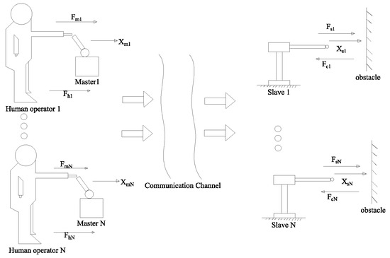
Figure 1. The structure diagram of the multilateral teleoperation system.

Substitute $F_{ji}$ into System (1), so that System (1) can be re-represented as

$$\begin{array}{c}{M}_{mi}\left(q_{mi}\right){\ddot{q}}_{mi}+C_{mi}(q_{mi},{\dot{q}}_{mi}){\dot{q}}_{mi}=u_{mi}^F+F_{hi},\hfill \\ M_{si}\left(q_{si}\right){\ddot{q}}_{si}+C_{si}(q_{si},{\dot{q}}_{si}){\dot{q}}_{si}=u_{si}^F-F_{ei}.\hfill \end{array}$$

(2)

For simplicity, consider that the multilateral teleoperation system consists of N master robots and N slave robots, both of which have two degrees of freedom. The configuration of a two-link robot is displayed in Figure 2, where $m_{jia}(a=1,2)$ represents the link massed, and $j=\{m,s\}$, $i=\{1,\cdots ,N\}$. $l_{in}(n=1,2)$ denotes the link lengths [26].

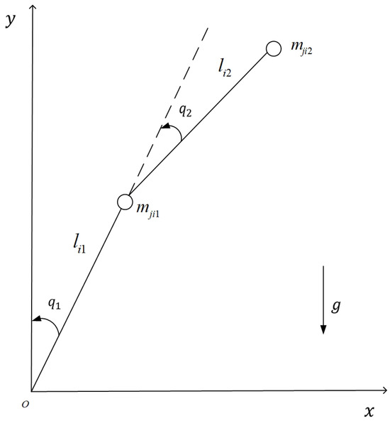
Figure 2. The configuration of a two-link robot.

As in [4,27,28], we define $x_{ji1}=q_{ji1}$, $x_{ji2}=q_{ji2}$, $x_{ji3}={\dot{q}}_{ji1}$ and $x_{ji4}={\dot{q}}_{ji2}$. Then, System (2) can be described as

$$\begin{array}{c}{\dot{x}}_{mi}\left(t\right)=f\left(x_{mi}\right)+\beta \left(x_{mi}\right)(u_{mi}^F+F_{hi})\hfill \\ {\dot{x}}_{si}\left(t\right)=f\left(x_{si}\right)+\beta \left(x_{si}\right)(u_{si}^F-F_{ei})\hfill \end{array}$$

(3)

where

$$\begin{array}{cc}\hfill f\left(x_{ji}\right)=& \left[\begin{array}{c}{x}_{ji3}\\ x_{ji4}\\ f_{i1}\left(x_{ji}\right)\\ f_{i2}\left(x_{ji}\right)\end{array}\right],\beta \left(x_{ji}\right)=\left[\begin{array}{cc}0& 0\\ 0& 0\\ {\beta }_{i1}\left(x_{ji}\right)& {\beta }_{i2}\left(x_{ji}\right)\\ {\beta }_{i2}\left(x_{ji}\right)& {\beta }_{i3}\left(x_{ji}\right)\end{array}\right],\hfill \end{array}$$

and

$$\begin{array}{cc}\hfill x_{ji}=& {\left[x_{ji1}^T{x}_{ji2}^T{x}_{ji3}^T{x}_{ji4}^T\right]}^T,u_{ji}^F=\left[\begin{array}{c}{u}_{ji1}^F\\ u_{ji2}^F\end{array}\right],\hfill \end{array}$$

$$\begin{array}{cc}\hfill f_{i1}\left(x_{ji}\right)=& {\displaystyle \frac{{\tilde{\aleph }}_{i1}\left[m_{ji2}{l}_{i1}{l}_{i2}{\tilde{\aleph }}_{i2}{x}_{ji3}^2-m_{ji2}{l}_{i2}^2{x}_{ji4}^2\right]}{l_{i1}{l}_{i2}\left[(m_{ji1}+m_{ji2})-m_{ji2}{\tilde{\aleph }}_{i2}^2\right]}},\hfill \\ \hfill f_{i2}\left(x_{ji}\right)=& {\displaystyle \frac{{\tilde{\aleph }}_{i1}\left[-(m_{ji1}+m_{ji2})l_{i1}^2{x}_{ji3}^2+m_{ji2}{l}_{i1}{l}_{i2}{\tilde{\aleph }}_{i2}{x}_{ji4}^2\right]}{l_{i1}{l}_{i2}\left[(m_{ji1}+m_{ji2})-m_{ji2}{\tilde{\aleph }}_{i2}^2\right]}},\hfill \\ \hfill {\beta }_{i1}\left(x_{ji}\right)=& {\displaystyle \frac{m_{ji2}{l}_{i2}^2}{m_{ji2}{l}_{i1}^2{l}_{i2}^2\left[(m_{ji1}+m_{ji2})-m_{ji2}{\tilde{\aleph }}_{i2}^2\right]}},\hfill \\ \hfill {\beta }_{i2}\left(x_{ji}\right)=& {\displaystyle \frac{-m_{ji2}{l}_{i1}{l}_{i2}{\tilde{\aleph }}_{i2}}{m_{ji2}{l}_{i1}^2{l}_{i2}^2\left[(m_{ji1}+m_{ji2})-m_{ji2}{\tilde{\aleph }}_{i2}^2\right]}},\hfill \\ \hfill {\beta }_{i3}\left(x_{ji}\right)=& {\displaystyle \frac{(m_{ji1}+m_{ji2})l_{i1}^2}{m_{ji2}{l}_{i1}^2{l}_{i2}^2\left[(m_{ji1}+m_{ji2})-m_{ji2}{\tilde{\aleph }}_{i2}^2\right]}},\hfill \\ \hfill {\tilde{\aleph }}_{i1}=& sin\left(x_{ji1}\right)cos\left(x_{ji2}\right)-cos\left(x_{ji1}\right)sin\left(x_{ji2}\right),\hfill \\ \hfill {\tilde{\aleph }}_{i2}=& sin\left(x_{ji1}\right)sin\left(x_{ji2}\right)+cos\left(x_{ji1}\right)cos\left(x_{ji2}\right).\hfill \end{array}$$

In practice, partial actuator failure is one of the important factors leading to system instability. As in [17,29], the application of fault-tolerant control is an appropriate way to solve partial actuator failures. The controller is designed as $u^F\left(t\right)=Mu\left(t\right)$, where

$$M=diag\{m_1,m_2,\dots ,m_p\}$$

denotes the partial actuator failure coefficients, which satisfy

$$\begin{array}{cc}& 0<m_v^{min}⩽m_v⩽m_v^{max}⩽1,v=1,2,\dots ,p.\hfill \end{array}$$

There are two cases: when $0<m_v<1$, it means that the ith actuator has partial failure; when $m_v=1$, the ith actuator is operating normally. It is worth noting that in the above failure description, the failure distribution is the same. However, in practice, the distribution of failures is different, and minor failures are always more probably to occur than serious failures. In other words, select an appropriate scalar ${\tilde{m}}_v$ in the interval $\left[m_v^{min},m_v^{max}\right]$ to divide the interval into two subintervals as $\left[m_v^{min},{\tilde{m}}_v\right)$, $\left[{\tilde{m}}_v,m_v^{max}\right]$. From the failure features, majority of the actuator failures fall under the interval $\left[{\tilde{m}}_v,m_v^{max}\right]$ as minor failures. The serious failure occurs at a low probability, which belongs to the interval $\left[{\tilde{m}}_v^{min},{\tilde{m}}_v\right]$. Due to the characteristic of partial actuator failures, the failure matrix can be redefined as

$$\begin{array}{c}\begin{array}{c}\widehat{M}=diag\{{\theta }_1\left(k\right)m_1+(1-{\theta }_1\left(k\right)){\overline{m}}_1,\dots ,{\theta }_p\left(k\right)m_p\hfill \\ +(1-{\theta }_p\left(k\right)){\overline{m}}_p\},\hfill \end{array}\hfill \end{array}$$

(4)

where

$$\begin{array}{cc}& m_v^{min}⩽m_v⩽{\tilde{m}}_v,{\theta }_v\left(k\right)=1\\ & {\tilde{m}}_v⩽{\overline{m}}_v⩽m_v^{max},{\theta }_v\left(k\right)=0\end{array},v=1,2,\dots ,p.$$

${\theta }_v\left(k\right)(v=1,\dots ,p)$ belongs to the set $[0,1]$ and is a random variable. In this research, the distribution probability of ${\theta }_v\left(k\right)$ is defined as $Prob\{{\theta }_v\left(k\right)=1\}={\tilde{\theta }}_v$, and it obeys the Bernoulli distribution. According to the novel failure matrix with failure distributions (4) of the above design, the fault-tolerant controllers can be defined as

$$u_{mi}^F\left(t\right)={\widehat{M}}_{mi}{u}_{mi}\left(t\right),u_{si}^F\left(t\right)={\widehat{M}}_{si}{u}_{si}\left(t\right),$$

(5)

where

$$\begin{array}{c}\hfill \begin{array}{c}{\widehat{M}}_{mi}=diag\{{\theta }_{1mi}\left(k\right)m_{1mi}+(1-{\theta }_{1mi}\left(k\right)){\overline{m}}_{1mi},\hfill \\ \dots ,{\theta }_{pmi}\left(k\right)m_{pmi}+(1-{\theta }_{pmi}\left(k\right)){\overline{m}}_{pmi}\},\hfill \\ {\widehat{M}}_{si}=diag\{{\theta }_{1si}\left(k\right)m_{1si}+(1-{\theta }_{1si}\left(k\right)){\overline{m}}_{1si},\hfill \\ \dots ,{\theta }_{psi}\left(k\right)m_{psi}+(1-{\theta }_{psi}\left(k\right)){\overline{m}}_{psi}\}\hfill \end{array}\end{array}$$

In this paper, $u_{mi}\left(t\right)$ and $u_{si}\left(t\right)$ are the nominal controllers to be contrived. Obviously, due to System (3) being a kind of nonlinear system with actuator failure, it is difficult to design the corresponding fault-tolerant controller directly for such a system. In order to solve this problem, the nonlinear system (System 3) is modeled as a Takagi–Sugeno (T-S) fuzzy system, and some fuzzy IF-THEN rules can be used to describe it. Among them, the fuzzy rules ($a^{th}$) regarding the master robot can be written as

$$\begin{array}{c}\hfill \begin{array}{c}IF{y}_{i1}\left(t\right)is{\Psi }_{ia1}and\dots and{y}_{ip}\left(t\right)is{\Psi }_{iap},\hfill \\ THEN{\dot{x}}_{mi}\left(t\right)=A_{mia}{x}_{mi}\left(t\right)+B_{mia}(u_{mi}^F\left(t\right)+F_{hi}\left(t\right)),\hfill \\ a=1,2,3,\dots ,L,\hfill \end{array}\end{array}$$

where ${\Psi }_{iab}$ denotes the fuzzy set, L represents the number of IF-THEN rules, and $y_{i1}\left(t\right),\cdots ,y_{ip}\left(t\right)$ are the premise variables. From this, the fuzzy system of the master manipulator can be deduced as follows:

$${\dot{x}}_{mi}\left(t\right)={\displaystyle \frac{{\displaystyle \sum _{a=1}^L}{\mu }_{ia}\left(y_i\left(t\right)\right)\left[A_{mia}{x}_{mi}\left(t\right)+B_{mia}(u_{mi}^F\left(t\right)+F_{hi}\left(t\right))\right]}{{\displaystyle \sum _{a=1}^L}{\mu }_{ia}\left(y_i\left(t\right)\right)}},$$

(6)

where

$${\mu }_{ia}\left(y_i\left(t\right)\right)=\prod _{b=1}^p{\Psi }_{iab}\left(y_i\left(t\right)\right),y_i\left(t\right)=\left[y_{i1}\left(t\right)y_{i2}\left(t\right)\dots y_{ip}\left(t\right)\right].$$

We assume that ${\mu }_{ia}\left(y_i\left(t\right)\right)⩾0$ and ${\sum }_{a=1}^L{\mu }_{ia}\left(y_i\left(t\right)\right)⩾0$. Denoting $h_{ia}\left(y_i\left(t\right)\right)={\mu }_{ia}\left(y_i\left(t\right)\right)$/ ${\sum }_{a=1}^L{\mu }_{ia}\left(y_i\left(t\right)\right)$, it is obvious to infer that $h_{ia}\left(y_i\left(t\right)\right)⩾0$ for $a=1,2,\dots ,L$ and ${\sum }_{a=1}^L{h}_{ia}\left(y_i\left(t\right)\right)=1$. Thus, the model of the master manipulator can be depicted as

$$\begin{array}{c}{\dot{x}}_{mi}\left(t\right)={\displaystyle \sum _{a=1}^L}{h}_{ia}\left(y_i\left(t\right)\right)\hfill \\ \times \left[A_{mia}{x}_{mi}\left(t\right)+B_{mia}(u_{mi}^F\left(t\right)+F_{hi}\left(t\right))\right].\hfill \end{array}$$

(7)

Similarly, the slave manipulator can be modeled as

$$\begin{array}{c}{\dot{x}}_{si}\left(t\right)={\displaystyle \sum _{a=1}^L}{h}_{ia}\left({\tilde{y}}_i\left(t\right)\right)\hfill \\ \times \left[A_{sia}{x}_{si}\left(t\right)+B_{sia}(u_{si}^F\left(t\right)-F_{ei}\left(t\right))\right].\hfill \end{array}$$

(8)

For the fuzzy model of the master manipulator (7), select one of the following fuzzy controllers, as follows:

Control Rule k:

$$\begin{array}{cc}& IF{y}_{i1}\left(t\right)is{\Psi }_{ik1}and\dots and{y}_{ip}\left(t\right)is{\Psi }_{ikp},\hfill \\ & THEN\hfill \\ & u_{mi}\left(t\right)=K_{mik}\left[x_{mi}\left(t\right)-\sum _{v=1}^N{\beta }_{vi}{x}_{svi}(t-d_{svi}\left(t\right))\right]\hfill \\ & -F_{ei}(t-d_{sii}\left(t\right))\hfill \end{array}$$

where $k=1,2,\dots ,L$. Then, the nominal fuzzy logic controller for the master manipulator (7) is obtained as

$$\begin{array}{c}\hfill \begin{array}{c}{u}_{mi}\left(t\right)={\displaystyle \sum _{k=1}^L}{h}_{ik}\left(y_i\left(t\right)\right)K_{mik}\hfill \\ \times \left[x_{mi}\left(t\right)-{\displaystyle \sum _{v=1}^N}{\beta }_{vi}{x}_{svi}(t-d_{svi}\left(t\right))\right]\hfill \\ -F_{ei}(t-d_{sii}\left(t\right))\hfill \end{array}\end{array}$$

(9)

Similarly, for slave manipulator (8), the nominal fuzzy controller is given as

$$\begin{array}{c}{u}_{si}\left(t\right)={\displaystyle \sum _{k=1}^L}{h}_{ik}\left({\tilde{y}}_i\left(t\right)\right)K_{sik}(x_{si}\left(t\right)-x_{mi}(t-d_{mi}\left(t\right)))\hfill \\ +F_{hi}(t-d_{mi}\left(t\right))\hfill \end{array}$$

(10)

Remark 1.

Here, the position tracking errors between the master manipulators and slave manipulators are defined as

$$\begin{array}{c}\hfill \begin{array}{c}{e}_{mi}\left(t\right)=x_{mi}\left(t\right)-{\displaystyle \sum _{v=1}^N}{\beta }_{vi}{x}_{svi}(t-d_{svi}\left(t\right))\hfill \\ e_{si}\left(t\right)=x_{si}\left(t\right)-x_{mi}(t-d_{mi}\left(t\right))\hfill \end{array}\end{array}$$

where ${\beta }_{vi}$ are the dominance factors having values in $(0,1)$ (see [30]), and ${\displaystyle \sum _{v=1}^N}{\beta }_{vi}=1$. The position synchronization of the masters and slaves could be achieved, i.e., ${lim}_{t\to 0}∥e_{mi}\left(t\right)∥=0$ and ${lim}_{t\to 0}∥e_{si}\left(t\right)∥=0$.

Assumption 1.

We assume that $d_{mi}\left(t\right)$ denotes the delay from master i to slave i, and $d_{svi}\left(t\right)$ denotes the delay from slave v to master i. Here, it is assumed that the communication delay of each pair of master–slave manipulators is asymmetrically and continuously differentiable functions, satisfying

$$\begin{array}{c}\hfill \left(\mathrm{i}\right)0\le d_{mi}\left(t\right)\le {\widehat{d}}_{mi}\left(\mathrm{ii}\right)0\le d_{svi}\left(t\right)\le {\widehat{d}}_{si}\end{array}$$

in which ${\dot{d}}_{mi}\left(t\right)\le \mu <1$, ${\dot{d}}_{svi}\left(t\right)\le \mu <1$. Additionally, μ, ${\widehat{d}}_{mi}$, and ${\widehat{d}}_{si}$ are positive scalars.

Substituting Equations (5) and (9) into Equation (7), it follows that

$$\begin{array}{c}\hfill \begin{array}{c}{\dot{x}}_{mi}\left(t\right)={\displaystyle \sum _{a=1}^L}{\displaystyle \sum _{k=1}^L}{h}_{ia}\left(y_i\left(t\right)\right)h_{ik}\left(y_i\left(t\right)\right)\hfill \\ \times [(A_{mia}+B_{mia}{\widehat{M}}_{mi}{K}_{mik})x_{mi}\left(t\right)\hfill \\ -{\displaystyle \sum _{v=1}^N}{\beta }_{vi}{B}_{mia}{\widehat{M}}_{mi}{K}_{mik}{x}_{svi}(t-d_{svi}\left(t\right))\hfill \\ -B_{mia}{\widehat{M}}_{mi}{F}_{ei}(t-d_{si}\left(t\right))+B_{mia}{F}_{hi}\left(t\right)].\hfill \end{array}\end{array}$$

(11)

Similarly, the following results can be derived from Equations (5), (8), and (10):

$$\begin{array}{c}\hfill \begin{array}{c}{\dot{x}}_{si}\left(t\right)={\displaystyle \sum _{a=1}^L}{\displaystyle \sum _{k=1}^L}{h}_{ia}\left({\tilde{y}}_i\left(t\right)\right)h_{ik}\left({\tilde{y}}_i\left(t\right)\right)\hfill \\ \times [(A_{sia}+B_{sia}{\widehat{M}}_{si}{K}_{sik})x_{si}\left(t\right)\hfill \\ -B_{sia}{\widehat{M}}_{si}{K}_{sik}{x}_{mi}(t-d_{mi}\left(t\right))\hfill \\ -B_{sia}{F}_{ei}\left(t\right)+B_{sia}{\widehat{M}}_{si}{F}_{hi}(t-d_{mi}\left(t\right))].\hfill \end{array}\end{array}$$

(12)

Assuming that all the premise variables of the master manipulators and the slave manipulators are the same, one can obtain

$$\begin{array}{c}\hfill \begin{array}{c}{\dot{\widehat{x}}}_i\left(t\right)={\displaystyle \sum _{a=1}^L}{\displaystyle \sum _{k=1}^L}{h}_{ia}\left(y_i\left(t\right)\right)h_{ik}\left(y_i\left(t\right)\right)\{{\widehat{A}}_{iak}{\widehat{x}}_i\left(t\right)\hfill \\ +{\displaystyle \sum _{v=1}^N}{\widehat{A}}_{1iakv}{\widehat{x}}_i(t-d_{svi}\left(t\right))+{\widehat{A}}_{2iak}{\widehat{x}}_i(t-d_{mi}\left(t\right))\hfill \\ +{\widehat{E}}_{ia}\widehat{\omega }\left(t\right)\},\hfill \end{array}\end{array}$$

(13)

where

$$\begin{array}{c}\hfill \begin{array}{c}{\widehat{A}}_{iak}=\left[\begin{array}{cc}{A}_{mia}+B_{mia}{\widehat{M}}_{mi}{K}_{mik}& 0\\ 0& A_{sia}+B_{sia}{\widehat{M}}_{si}{K}_{sik}\end{array}\right],\hfill \\ {\widehat{x}}_i\left(t\right)=\left[\begin{array}{c}{x}_{mi}\left(t\right)\\ x_{si}\left(t\right)\end{array}\right],{\widehat{A}}_{1iakv}=\left[\begin{array}{cc}0& 0\\ 0& -{\beta }_{vi}{B}_{mia}{\widehat{M}}_{mi}{K}_{mik}\end{array}\right],\hfill \\ {\widehat{A}}_{2iak}=\left[\begin{array}{cc}-B_{sia}{\widehat{M}}_{si}{K}_{sik}& 0\\ 0& 0\end{array}\right],{\widehat{E}}_{ia}=\left[\begin{array}{cc}{B}_{mia}& 0\\ 0& B_{sia}\end{array}\right],\hfill \\ \widehat{\omega }\left(t\right)=\left[\begin{array}{c}{F}_{hi}\left(t\right)-{\widehat{M}}_{mi}{F}_{ei}(t-d_{si}\left(t\right))\\ {\widehat{M}}_{si}{F}_{hi}(t-d_{mi}\left(t\right))-F_{ei}\left(t\right)\end{array}\right].\hfill \end{array}\end{array}$$

A new variable $z_i\left(t\right)$ is defined as the controlled output:

$$z_i\left(t\right)=x_{mi}\left(t\right)-x_{si}\left(t\right)=\left[I-I\right]{\widehat{x}}_i\left(t\right)=\widehat{C}{\widehat{x}}_i\left(t\right).$$

(14)

Before construing the closed-loop system stability of Equations (13) and (14), basic lemmas are introduced beforehand, as follows:

Lemma 1

([31]). For any symmetric constant matrix $M>0$, as well as scalars α and β satisfying $\beta >\alpha$, a vector function ω: $[\alpha ,\beta ]\to {\mathbb{R}}^n$, such that the integration concerned exists; thus,

$$\begin{array}{c}(\beta -\alpha ){\int }_{\alpha }^{\beta }{\omega }^T\left(s\right)M\omega \left(s\right)ds\hfill \\ \ge {\left[{\int }_{\alpha }^{\beta }\omega \left(s\right)ds\right]}^{T}M\left[{\int }_{\alpha }^{\beta }\omega \left(s\right)ds\right].\hfill \end{array}$$

Lemma 2

([32]). Let $L=L^T$, M and N be real symmetric matrices of suitable dimensions with $F\left(t\right)$ satisfying $F^T\left(t\right)F\left(t\right)⩽I$, then the following inequality holds:

$$L+MF\left(t\right)N+N^{T}F{\left(t\right)}^T{M}^T<0,$$

if and only if there exists a scalar $\sigma >0$, such that

$$L+{\sigma }^{-1}M{M}^T+\sigma N^{T}N<0.$$

Lemma 3

(Schur complement: [33]). Given a symmetric matrix

$$S=\left[\begin{array}{cc}{S}_{11}& S_{12}\\ S_{12}^T& S_{22}\end{array}\right],$$

the following statements are equivalent:

$$\begin{array}{cc}& \left(1\right)S<0;\hfill \\ & \left(2\right)S_{11}<0,S_{22}-S_{12}^T{S}_{11}^{-1}{S}_{12}<0;\hfill \\ & \left(3\right)S_{22}<0,S_{11}-S_{12}{S}_{22}^{-1}{S}_{12}^T<0.\hfill \end{array}$$

Main Results

In this section, the stability of the closed-loop systems (13), and (14) will be examinated. The issue will be depicted in more detail, as follows: on the premise of ensuring the mean square stability of the system (13) with a predefined $H_{\infty }$ performance requirement, a suitable $H_{\infty }$ fault-tolerant controller is designed.

1. The system (13) is a mean-square stable system with $\widehat{\omega }\left(t\right)=0$.

2. Under the premise of the initial condition being zero and given a noise attenuation level $\gamma$, the system can live up to the following performance requirements.

$$\mathbb{E}\left\{{\int }_0^{\infty }{z}^T\left(t\right)z\left(t\right)dt\right\}<\mathbb{E}\left\{{\gamma }^2{\int }_0^{\infty }{\widehat{\omega }}^T\left(t\right)\widehat{\omega }\left(t\right)dt\right\}.$$

The first result is obtained as follows:

Theorem 1.

For positive scalar $\gamma >0$, there exist positive definite symmetrical matrices $P_i>0$, $Q_{svi}>0$, $Q_{mi}>0$, $W_{si}>0$, $W_{mi}>0$, and matrix N with suitable dimensions. Given the appropriate controller gains $K_{mik}$ and $K_{sik}$, $k=1,2,\cdots ,L$, as well as matrices ${\tilde{M}}_{mi}$ and ${\tilde{M}}_{si}$, the following linear matrix inequality is satisfied, and then the closed-loop system (13) is a mean-square stable system with an $H_{\infty }$ disturbance attenuation level γ.

$$\tilde{\Xi }=\left[\begin{array}{cccc}{\Phi }_1& {\Phi }_2& {\Phi }_3& {\Phi }_4\\ *& {\Phi }_5& 0& 0\\ *& *& -{\gamma }^{2}I& 0\\ *& *& *& -{\gamma }^{2}I\end{array}\right]<0,$$

(15)

where

$$\begin{array}{c}\hfill \begin{array}{c}{\Phi }_1=\left[\begin{array}{cccccc}{\Phi }_{11}& {\Phi }_{12}& {\Phi }_{13}& -P_i& 0& 0\\ *& {\Phi }_{22}& -P_i& {\Phi }_{23}& 0& {\Phi }_{24}\\ *& *& {\Phi }_{33}& {\Phi }_{34}& 0& 0\\ *& *& *& {\Phi }_{33}& 0& {\Phi }_{24}\\ *& *& *& *& {\Phi }_{55}& {\Phi }_{56}\\ *& *& *& *& *& {\Phi }_{55}\end{array}\right],\hfill \\ {\Phi }_2=\left[\begin{array}{cccccc}{\Phi }_{14}& 0& W_{si}& -W_{si}& W_{mi}& -W_{mi}\\ 0& 0& -W_{si}& W_{si}& -W_{mi}& W_{mi}\\ {\Phi }_{14}& 0& 0& 0& 0& 0\\ 0& 0& 0& 0& 0& 0\\ 0& 0& 0& 0& 0& 0\\ 0& 0& 0& 0& 0& 0\end{array}\right],\hfill \\ {\Phi }_3={\left[\begin{array}{cccccc}{B}_{mia}^T{N}^T& 0& B_{mia}^T{N}^T& 0& 0& 0\end{array}\right]}^T,\hfill \\ {\Phi }_4={\left[\begin{array}{cccccc}0& B_{sia}^T{N}^T& 0& B_{sia}^T{N}^T& 0& 0\end{array}\right]}^T,\hfill \end{array}\end{array}$$

$$\begin{array}{c}\hfill \begin{array}{c}{\Phi }_5=\left[\begin{array}{cccccc}{\Phi }_{57}& {\Phi }_{58}& 0& 0& 0& 0\\ *& {\Phi }_{57}& 0& 0& 0& 0\\ *& *& -W_{si}& W_{si}& 0& 0\\ *& *& *& -W_{si}& 0& 0\\ *& *& *& *& -W_{mi}& W_{mi}\\ *& *& *& *& *& -W_{mi}\end{array}\right],\hfill \\ {\Phi }_{11}={\beta }_{vi}{Q}_{svi}+Q_{mi}-W_{si}-W_{mi}+I\hfill \\ +\mathbf{He}(N{A}_{mia}+N{B}_{mia}{\tilde{M}}_{mi}{K}_{mik}),\hfill \\ {\Phi }_{12}=-{\beta }_{vi}{Q}_{svi}-Q_{mi}+W_{si}+W_{mi}-I,\hfill \\ {\Phi }_{14}=-N{B}_{sia}{\tilde{M}}_{si}{K}_{sik},\hfill \\ {\Phi }_{13}=P_i-N+N{A}_{mia}+N{B}_{mia}{\tilde{M}}_{mi}{K}_{mik},\hfill \\ {\Phi }_{22}={\beta }_{vi}{Q}_{svi}+Q_{mi}-W_{si}-W_{mi}+I\hfill \\ +\mathbf{He}(N{A}_{sia}+N{B}_{sia}{\tilde{M}}_{si}{K}_{sik}),\hfill \\ {\Phi }_{23}=P_i-N+N{A}_{sia}+N{B}_{sia}{\tilde{M}}_{si}{K}_{sik},\hfill \\ {\Phi }_{24}=-{\beta }_{vi}N{B}_{mia}{\tilde{M}}_{mi}{K}_{mik},\hfill \\ {\Phi }_{33}={\widehat{d}}_{si}^2{W}_{si}+{\widehat{d}}_{mi}^2{W}_{mi}-\mathbf{He}\left(N\right),\hfill \\ {\Phi }_{34}=-{\widehat{d}}_{si}^2{W}_{si}-{\widehat{d}}_{mi}^2{W}_{mi},\hfill \\ {\Phi }_{55}=-(1-\mu ){\beta }_{vi}{Q}_{svi},{\Phi }_{56}=(1-\mu ){\beta }_{vi}{Q}_{svi},\hfill \\ {\Phi }_{57}=-(1-\mu )Q_{mi},{\Phi }_{58}=(1-\mu )Q_{mi}.\hfill \end{array}\end{array}$$

Proof. 

The following Lyapunov–Krasovskii functions can be considered:

$$\begin{array}{c}\hfill \begin{array}{c}V\left(t\right)=V_1\left(t\right)+V_2\left(t\right)+V_3\left(t\right),\hfill \\ V_1\left(t\right)={\displaystyle \sum _{i=1}^N}{z}_i^T\left(t\right)P_i{z}_i\left(t\right),\hfill \end{array}\end{array}$$

$$\begin{array}{c}\hfill \begin{array}{c}{V}_2\left(t\right)={\displaystyle \sum _{i=1}^N}\left\{{\displaystyle \sum _{v=1}^N}{\beta }_{vi}{\int }_{t-d_{svi}\left(t\right)}^t{z}_i^T\left(\varphi \right)\right.Q_{svi}{z}_i\left(\varphi \right)d\varphi \hfill \\ +{\widehat{d}}_{si}\left.{\int }_{t-{\widehat{d}}_{si}}^t{\int }_{t+\sigma }^t{\dot{z}}_i^T\left(\varphi \right)W_{si}{\dot{z}}_i\left(\varphi \right)d\varphi d\sigma \right\},\hfill \\ V_3\left(t\right)={\displaystyle \sum _{i=1}^N}\left\{{\int }_{t-d_{mi}\left(t\right)}^t{z}_i^T\left(\varphi \right)Q_{mi}{z}_i\left(\varphi \right)d\varphi \right.\hfill \\ +\left.{\widehat{d}}_{mi}{\int }_{t-{\widehat{d}}_{mi}}^t{\int }_{t+\sigma }^t{\dot{z}}_i^T\left(\varphi \right)W_{mi}{z}_i\left(\varphi \right)d\varphi d\sigma \right\}.\hfill \end{array}\end{array}$$

(16)

Then, the differentiation of $V\left(t\right)$ can be described as

$$\begin{array}{c}\hfill \begin{array}{c}\mathbb{E}\left\{{\dot{V}}_1\left(t\right)\right\}=\mathbb{E}\left\{{\displaystyle \sum _{i=1}^N}2z_i^T\left(t\right)P_i{\dot{z}}_i\left(t\right)\right\},\hfill \\ \mathbb{E}\left\{{\dot{V}}_2\left(t\right)\right\}=\mathbb{E}\{{\displaystyle \sum _{i=1}^N}{\displaystyle \sum _{v=1}^N}[{\beta }_{vi}{z}_i^T\left(t\right)Q_{svi}{z}_i\left(t\right)\hfill \\ -{\beta }_{vi}(1-{\dot{d}}_{svi}\left(t\right))z_i^T(t-d_{svi}\left(t\right))\hfill \\ \times Q_{svi}{z}_i(t-d_{svi}\left(t\right))\left]\right\}\hfill \\ +\mathbb{E}\{{\displaystyle \sum _{i=1}^N}[{\widehat{d}}_{si}^2{\dot{z}}_i^T\left(t\right)W_{si}{\dot{z}}_i\left(t\right)\hfill \\ -{\widehat{d}}_{si}{\int }_{t-{\widehat{d}}_{si}}^t{\dot{z}}_i^T\left(\sigma \right)W_{si}{\dot{z}}_i\left(\sigma \right)d\sigma \left]\right\},\hfill \\ \mathbb{E}\left\{{\dot{V}}_3\left(t\right)\right\}=\mathbb{E}\{{\displaystyle \sum _{i=1}^N}[z_i^T\left(t\right)Q_{mi}{z}_i\left(t\right)\hfill \\ -(1-{\dot{d}}_{mi}\left(t\right))z_i^T(t-d_{mi}\left(t\right))\hfill \\ \times Q_{mi}{z}_i(t-d_{mi}\left(t\right))\hfill \\ +{\widehat{d}}_{mi}^2{\dot{z}}_i^T\left(t\right)W_{mi}{\dot{z}}_i\left(t\right)\hfill \\ -{\widehat{d}}_{mi}{\int }_{t-{\widehat{d}}_{mi}}^t{\dot{z}}_i^T\left(\sigma \right)W_{mi}{\dot{z}}_i\left(\sigma \right)d\sigma \left]\right\}.\hfill \end{array}\end{array}$$

(17)

Under the premise of the time-varying delay assumed above, using Lemma 1 yields

$$\begin{array}{c}\hfill \begin{array}{c}\mathbb{E}\left\{\dot{V}\left(t\right)\right\}\le \mathbb{E}\{{\displaystyle \sum _{i=1}^N}[2z_i^T\left(t\right)P_i{\dot{z}}_i\left(t\right)+z_i^T\left(t\right){\displaystyle \sum _{v=1}^N}{\beta }_{vi}{Q}_{svi}{z}_i\left(t\right)\hfill \\ +{\widehat{d}}_{si}^2{\dot{z}}_i^T\left(t\right)W_{si}{\dot{z}}_i\left(t\right)+z_i^T\left(t\right)Q_{mi}{z}_i\left(t\right)\hfill \\ -(1-\mu )z_i^T(t-d_{svi}\left(t\right))\hfill \\ \times {\displaystyle \sum _{v=1}^N}{\beta }_{vi}{Q}_{svi}{z}_i(t-d_{svi}\left(t\right))\hfill \\ -{(z_i\left(t\right)-z_i(t-{\widehat{d}}_{si}))}^T{W}_{si}(z_i\left(t\right)-z_i(t-{\widehat{d}}_{si}))\hfill \\ +{\widehat{d}}_{mi}^2{\dot{z}}_i^T\left(t\right)W_{mi}{\dot{z}}_i\left(t\right)\hfill \\ -(1-\mu )z_i^T(t-d_{mi}\left(t\right))Q_{mi}{z}_i(t-d_{mi}\left(t\right))\hfill \\ -{(z_i\left(t\right)-z_i(t-{\widehat{d}}_{mi}))}^T\hfill \\ \times W_{mi}(z_i\left(t\right)-z_i(t-{\widehat{d}}_{mi}))\left]\right\}.\hfill \end{array}\end{array}$$

(18)

By substituting Equation (14) into (18), it follows that

$$\begin{array}{c}\hfill \begin{array}{c}\mathbb{E}\left\{\dot{V}\left(t\right)\right\}\le \mathbb{E}\{{\displaystyle \sum _{i=1}^N}{\displaystyle \sum _{v=1}^N}[2{\widehat{x}}_i^T\left(t\right)\left[\begin{array}{cc}{P}_i& -P_i\\ -P_i& P_i\end{array}\right]{\dot{\widehat{x}}}_i^T\left(t\right)\hfill \\ +{\widehat{x}}_i^T\left(t\right)\left[\begin{array}{cc}{\beta }_{vi}{Q}_{svi}& -{\beta }_{vi}{Q}_{svi}\\ -{\beta }_{vi}{Q}_{svi}& {\beta }_{vi}{Q}_{svi}\end{array}\right]{\widehat{x}}_i\left(t\right)\hfill \\ +{\widehat{x}}_i^T(t-d_{svi}\left(t\right))\hfill \\ \times \left[\begin{array}{cc}-(1-\mu ){\beta }_{vi}{Q}_{svi}& (1-\mu ){\beta }_{vi}{Q}_{svi}\\ (1-\mu ){\beta }_{vi}{Q}_{svi}& -(1-\mu ){\beta }_{vi}{Q}_{svi}\end{array}\right]\hfill \\ \times {\widehat{x}}_i(t-d_{svi}\left(t\right))\hfill \\ +{\dot{\widehat{x}}}_i^T\left(t\right)\left[\begin{array}{cc}{\widehat{d}}_{si}^2{W}_{si}& -{\widehat{d}}_{si}^2{W}_{si}\\ -{\widehat{d}}_{si}^2{W}_{si}& {\widehat{d}}_{si}^2{W}_{si}\end{array}\right]{\dot{\widehat{x}}}_i^T\left(t\right)\hfill \end{array}\end{array}$$

$$\begin{array}{c}\hfill \begin{array}{c}+{({\widehat{x}}_i\left(t\right)-{\widehat{x}}_i(t-{\widehat{d}}_{si}))}^T\left[\begin{array}{cc}-W_{si}& W_{si}\\ W_{si}& -W_{si}\end{array}\right]\hfill \\ \times ({\widehat{x}}_i\left(t\right)-{\widehat{x}}_i(t-{\widehat{d}}_{si}))\hfill \\ +{\widehat{x}}_i^T\left(t\right)\left[\begin{array}{cc}{Q}_{mi}& -Q_{mi}\\ -Q_{mi}& Q_{mi}\end{array}\right]{\widehat{x}}_i\left(t\right)\hfill \\ +{\widehat{x}}_i^T(t-d_{mi}\left(t\right))\left[\begin{array}{cc}-(1-\mu )Q_{mi}& (1-\mu )Q_{mi}\\ (1-\mu )Q_{mi}& -(1-\mu )Q_{mi}\end{array}\right]\hfill \\ \times {\widehat{x}}_i(t-d_{mi}\left(t\right))\hfill \\ +{({\widehat{x}}_i\left(t\right)-{\widehat{x}}_i(t-{\widehat{d}}_{mi}))}^T\left[\begin{array}{cc}-W_{mi}& W_{mi}\\ W_{mi}& -W_{mi}\end{array}\right]\hfill \\ \times ({\widehat{x}}_i\left(t\right)-{\widehat{x}}_i(t-{\widehat{d}}_{mi}))\hfill \\ +{\dot{\widehat{x}}}_i^T\left(t\right)\left[\begin{array}{cc}{\widehat{d}}_{mi}^2{W}_{mi}& -{\widehat{d}}_{mi}^2{W}_{mi}\\ -{\widehat{d}}_{mi}^2{W}_{mi}& {\widehat{d}}_{mi}^2{W}_{mi}\end{array}\right]{\dot{\widehat{x}}}_i^T\left(t\right)\left]\right\}.\hfill \end{array}\end{array}$$

(19)

Using free-weight matrix technology yields

$$0=[{\widehat{x}}_i^T\left(t\right)\mathcal{N}+{\dot{\widehat{x}}}_i^T\left(t\right)\mathcal{N}]\mathcal{W}+{\mathcal{W}}^T[{\mathcal{N}}^T{\widehat{x}}_i\left(t\right)+{\mathcal{N}}^T{\dot{\widehat{x}}}_i^T\left(t\right)],$$

(20)

where

$$\begin{array}{c}\hfill \begin{array}{c}\mathcal{W}={\displaystyle \sum _{a=1}^L}{\displaystyle \sum _{k=1}^L}{h}_{ia}\left(y_i\left(t\right)\right)h_{ik}\left(y_i\left(t\right)\right)\{{\widehat{A}}_{iak}{\widehat{x}}_i\left(t\right)\hfill \\ +{\displaystyle \sum _{v=1}^N}{\widehat{A}}_{1iakv}{\widehat{x}}_i(t-d_{svi}\left(t\right))+{\widehat{A}}_{2iak}{\widehat{x}}_i(t-d_{mi}\left(t\right))\hfill \\ +{\widehat{E}}_{ia}\widehat{\omega }\left(t\right)\}-{\dot{\widehat{x}}}_i^T\left(t\right).\hfill \end{array}\end{array}$$

From the above Equations (19) and (20), one can induce that

$${\xi }^T\left(t\right)\Xi \xi \left(t\right)=0,$$

(21)

where

$$\begin{array}{c}\hfill \begin{array}{c}\xi \left(t\right)=[{\widehat{x}}_i^T\left(t\right){\dot{\widehat{x}}}_i^T\left(t\right){\widehat{x}}_i^T(t-d_{svi}\left(t\right)){\widehat{x}}_i^T(t-d_{mi}\left(t\right))\hfill \\ {\widehat{x}}_i^T(t-{\widehat{d}}_{si}){\widehat{x}}_i^T(t-{\widehat{d}}_{mi}){\widehat{\omega }}^T\left(t\right){]}^T.\hfill \end{array}\end{array}$$

Next, the system performance requirement can be structured, as follows:

$$\begin{array}{c}\hfill \begin{array}{c}J={\displaystyle \sum _{a=1}^L}{\displaystyle \sum _{k=1}^L}{h}_{ia}\left(y_i\left(t\right)\right)h_{ik}\left(y_i\left(t\right)\right)\mathbb{E}\{\dot{V}\left(t\right)\hfill \\ +z_i^T\left(t\right)z_i\left(t\right)-{\gamma }^2{\widehat{\omega }}^T\left(t\right)\widehat{\omega }\left(t\right)\}\hfill \\ \le {\displaystyle \sum _{a=1}^L}{\displaystyle \sum _{k=1}^L}{h}_{ia}\left(y_i\left(t\right)\right)h_{ik}\left(y_i\left(t\right)\right)\mathbb{E}\{{\xi }^T\left(t\right)\Xi \xi \left(t\right)\}.\hfill \end{array}\end{array}$$

Define

$$\begin{array}{c}\hfill \begin{array}{c}\mathcal{N}=\left[\begin{array}{cc}N& 0\\ 0& N\end{array}\right],\mathbb{E}\left\{{\widehat{M}}_{mi}\right\}={\tilde{M}}_{mi},\hfill \\ \mathbb{E}\left\{{\widehat{M}}_{si}\right\}={\tilde{M}}_{si},\mathbb{E}\{\Xi \}=\tilde{\Xi },\hfill \end{array}\end{array}$$

If $J<0$ holds, $\tilde{\Xi }<0$ in Equation (15) is naturally satisfied. Then, it follows that

$$\left[\begin{array}{cc}{\Phi }_1& {\Phi }_2\\ *& {\Phi }_5\end{array}\right]<0.$$

It is clear that the system (13) is a mean-square stable system with $\widehat{\omega }\left(t\right)=0$. In addition, Inequality (15) demonstrates that

$$\mathbb{E}\{\dot{V}\left(t\right)+z_i^T\left(t\right)z_i\left(t\right)-{\gamma }^2{\widehat{\omega }}^T\left(t\right)\widehat{\omega }\left(t\right)\}<0$$

(22)

holds. Furthermore, according to the initial condition of zero, by colligating both sides of Equation (22) from 0 to t and setting $t\to \infty$, one has

$$\mathbb{E}\left\{{\int }_0^{\infty }{z}_i^T\left(t\right)z_i\left(t\right)dt\right\}<\mathbb{E}\left\{{\int }_0^{\infty }{\gamma }^2{\widehat{\omega }}^T\left(t\right)\widehat{\omega }\left(t\right)dt\right\},$$

Thus, the performance requirement is achieved. This means that the system (13) is a mean-square stable system at the level $\gamma$ of interference attenuation $H_{\infty }$. □

Next, the second theorem derived from the first theorem is used to design the controller gains $K_{mik}$ and $K_{sik}$.

Theorem 2.

Given suitable matrices ${\tilde{M}}_{mi}$ and ${\tilde{M}}_{si}$, design the controller gains as $K_{mik}=Y_{mik}{\widehat{N}}^{-1}$, $K_{sik}=Y_{sik}{\widehat{N}}^{-1}$. For a positive scalar $\gamma >0$, there exist positive definite symmetrical matrices ${\widehat{P}}_i>0$, ${\widehat{Q}}_{svi}>0$, ${\widehat{Q}}_{mi}>0$, ${\widehat{W}}_{si}>0$, ${\widehat{W}}_{mi}>0$, and matrix $\widehat{N}$, $Y_{mik}$, $Y_{sik}$ with suitable dimensions; thus, the following linear matrix inequalities are satisfied, and then the closed-loop system (13) is a mean-square stable system with an $H_{\infty }$ disturbance attenuation level γ.

$${\tilde{\Xi }}_1=\left[\begin{array}{ccccc}{\tilde{\Phi }}_1& {\tilde{\Phi }}_2& {\tilde{\Phi }}_3& {\tilde{\Phi }}_4& {\tilde{\Phi }}_6\\ *& {\tilde{\Phi }}_5& 0& 0& 0\\ *& *& -{\gamma }^{2}I& 0& 0\\ *& *& *& -{\gamma }^{2}I& 0\\ *& *& *& *& -I\end{array}\right]<0,$$

(23)

where

$$\begin{array}{c}\hfill \begin{array}{c}{\tilde{\Phi }}_1=\left[\begin{array}{cccccc}{\tilde{\Phi }}_{11}& {\tilde{\Phi }}_{12}& {\tilde{\Phi }}_{13}& -{\widehat{P}}_i& 0& 0\\ *& {\tilde{\Phi }}_{22}& -{\widehat{P}}_i& {\tilde{\Phi }}_{23}& 0& {\tilde{\Phi }}_{24}\\ *& *& {\tilde{\Phi }}_{33}& {\tilde{\Phi }}_{34}& 0& 0\\ *& *& *& {\tilde{\Phi }}_{33}& 0& {\tilde{\Phi }}_{24}\\ *& *& *& *& {\tilde{\Phi }}_{55}& {\tilde{\Phi }}_{56}\\ *& *& *& *& *& {\tilde{\Phi }}_{55}\end{array}\right],\hfill \\ {\tilde{\Phi }}_3={\left[\begin{array}{cccccc}{B}_{mia}^T& 0& B_{mia}^T& 0& 0& 0\end{array}\right]}^T,\hfill \\ {\tilde{\Phi }}_4={\left[\begin{array}{cccccc}0& B_{sia}^T& 0& B_{sia}^T& 0& 0\end{array}\right]}^T,\hfill \end{array}\end{array}$$

$$\begin{array}{c}\hfill \begin{array}{c}{\tilde{\Phi }}_2=\left[\begin{array}{cccccc}{\tilde{\Phi }}_{14}& 0& W_{si}& -W_{si}& W_{mi}& -W_{mi}\\ 0& 0& -W_{si}& W_{si}& -W_{mi}& W_{mi}\\ {\tilde{\Phi }}_{14}& 0& 0& 0& 0& 0\\ 0& 0& 0& 0& 0& 0\\ 0& 0& 0& 0& 0& 0\\ 0& 0& 0& 0& 0& 0\end{array}\right],\hfill \\ {\tilde{\Phi }}_5=\left[\begin{array}{cccccc}{\tilde{\Phi }}_{57}& {\tilde{\Phi }}_{58}& 0& 0& 0& 0\\ *& {\tilde{\Phi }}_{57}& 0& 0& 0& 0\\ *& *& -{\widehat{W}}_{si}& {\widehat{W}}_{si}& 0& 0\\ *& *& *& -{\widehat{W}}_{si}& 0& 0\\ *& *& *& *& -{\widehat{W}}_{mi}& {\widehat{W}}_{mi}\\ *& *& *& *& *& -{\widehat{W}}_{mi}\end{array}\right],\hfill \\ {\tilde{\Phi }}_6={\left[\begin{array}{cccccc}\widehat{N}& -\widehat{N}& 0& 0& 0& 0\end{array}\right]}^T,\hfill \\ {\tilde{\Phi }}_{14}=-B_{sia}{\widehat{M}}_{si}{Y}_{sik},\hfill \\ {\tilde{\Phi }}_{11}={\beta }_{vi}{\widehat{Q}}_{svi}+{\widehat{Q}}_{mi}-{\widehat{W}}_{si}-{\widehat{W}}_{mi}\hfill \\ +\mathbf{He}(A_{mia}\widehat{N}+B_{mia}{\widehat{M}}_{mi}{Y}_{mik}),\hfill \\ {\tilde{\Phi }}_{12}=-{\beta }_{vi}{\widehat{Q}}_{svi}-{\widehat{Q}}_{mi}+{\widehat{W}}_{si}+{\widehat{W}}_{mi},\hfill \\ {\tilde{\Phi }}_{13}={\widehat{P}}_i-\widehat{N}+A_{mia}\widehat{N}+B_{mia}{\widehat{M}}_{mi}{Y}_{mik},\hfill \\ {\tilde{\Phi }}_{22}={\beta }_{vi}{\widehat{Q}}_{svi}+{\widehat{Q}}_{mi}-{\widehat{W}}_{si}-{\widehat{W}}_{mi}\hfill \\ +\mathbf{He}(A_{sia}\widehat{N}+B_{sia}{\widehat{M}}_{si}{Y}_{sik}),\hfill \\ {\tilde{\Phi }}_{23}={\widehat{P}}_i-\widehat{N}+A_{sia}\widehat{N}+B_{sia}{\widehat{M}}_{si}{Y}_{sik},\hfill \\ {\tilde{\Phi }}_{24}=-{\beta }_{vi}{B}_{mia}{\widehat{M}}_{mi}{Y}_{mik},\hfill \\ {\tilde{\Phi }}_{33}={\widehat{d}}_{si}^2{\widehat{W}}_{si}+{\widehat{d}}_{mi}^2{\widehat{W}}_{mi}-\mathbf{He}\left(\widehat{N}\right),\hfill \\ {\tilde{\Phi }}_{34}=-{\widehat{d}}_{si}^2{\widehat{W}}_{si}-{\widehat{d}}_{mi}^2{\widehat{W}}_{mi},\hfill \\ {\tilde{\Phi }}_{55}=-(1-\mu ){\beta }_{vi}{\widehat{Q}}_{svi},{\tilde{\Phi }}_{56}=(1-\mu ){\beta }_{vi}{\widehat{Q}}_{svi},\hfill \\ {\tilde{\Phi }}_{57}=-(1-\mu ){\widehat{Q}}_{mi},{\tilde{\Phi }}_{58}=(1-\mu ){\widehat{Q}}_{mi}.\hfill \end{array}\end{array}$$

Proof. 

We multiply $diag\{\stackrel{12}{\overbrace{{\widehat{N}}^T,\dots ,{\widehat{N}}^T}},I,I\}$ and $diag\{\stackrel{12}{\overbrace{\widehat{N},\dots ,\widehat{N}}},I,I\}$ on the left and right sides of $\tilde{\Xi }$ (15), respectively. Denoting ${\widehat{N}}^{T}N=I$, ${\widehat{P}}_i={\widehat{N}}^T{P}_i\widehat{N}$, ${\widehat{Q}}_{svi}={\widehat{N}}^T{Q}_{svi}\widehat{N}$, ${\widehat{Q}}_{mi}={\widehat{N}}^T{Q}_{mi}\widehat{N}$, ${\widehat{W}}_{si}={\widehat{N}}^T{W}_{si}\widehat{N}$, ${\widehat{W}}_{mi}={\widehat{N}}^T{W}_{mi}\widehat{N}$, the results listed below are derived:

$$\left[\begin{array}{cccc}{\tilde{\Phi }}_1& {\tilde{\Phi }}_2& {\tilde{\Phi }}_3& {\tilde{\Phi }}_4\\ *& {\tilde{\Phi }}_5& 0& 0\\ *& *& -{\gamma }^{2}I& 0\\ *& *& *& -{\gamma }^{2}I\end{array}\right]+\left[\begin{array}{c}{\tilde{\Phi }}_6\\ 0_{6\times 1}\end{array}\right]{\left[\begin{array}{cc}{\tilde{\Phi }}_6& 0_{1\times 6}\end{array}\right]}^T<0.$$

Through the Schur complement of Lemma 3, the corresponding result in Equation (23) is directly obtained. □

However, in Theorems 1 and 2, we assume that ${\tilde{M}}_{mi}$ and ${\tilde{M}}_{si}$ are already known, and they are represented as follows:

$$\begin{array}{c}\hfill \begin{array}{c}{\tilde{M}}_{mi}=diag\{{\tilde{\theta }}_{1mi}{m}_{1mi}+(1-{\tilde{\theta }}_{1mi}){\overline{m}}_{1mi},...,\hfill \\ {\tilde{\theta }}_{pmi}{m}_{pmi}+(1-{\tilde{\theta }}_{pmi}){\overline{m}}_{pmi}\},\hfill \\ {\tilde{M}}_{si}=diag\{{\tilde{\theta }}_{1si}{m}_{1si}+(1-{\tilde{\theta }}_{1si}){\overline{m}}_{1si},...,\hfill \\ {\tilde{\theta }}_{psi}{m}_{psi}+(1-{\tilde{\theta }}_{psi}){\overline{m}}_{psi}\}.\hfill \end{array}\end{array}$$

(24)

Define

$$\begin{array}{c}\hfill \begin{array}{c}{\tilde{\Theta }}_{mi}=diag\{{\tilde{\theta }}_{1mi},...,{\tilde{\theta }}_{pmi}\},{\tilde{\Theta }}_{si}=diag\{{\tilde{\theta }}_{1si},...,{\tilde{\theta }}_{psi}\},\hfill \\ {\Gamma }_{mi}=diag\{m_{1mi},...,m_{pmi}\},{\overline{\Gamma }}_{mi}=diag\{{\overline{m}}_{1mi},...,{\overline{m}}_{pmi}\},\hfill \\ {\Gamma }_{si}=diag\{m_{1si},...,m_{psi}\},{\overline{\Gamma }}_{si}=diag\{{\overline{m}}_{1si},...,{\overline{m}}_{psi}\},\hfill \end{array}\end{array}$$

and Equation (24) can be rewritten as

$$\begin{array}{c}\hfill \begin{array}{c}{\tilde{M}}_{mi}={\tilde{\Theta }}_{mi}{\Gamma }_{mi}+(1-{\tilde{\Theta }}_{mi}){\overline{\Gamma }}_{mi},\hfill \\ {\tilde{M}}_{si}={\tilde{\Theta }}_{si}{\Gamma }_{si}+(1-{\tilde{\Theta }}_{si}){\overline{\Gamma }}_{si}.\hfill \end{array}\end{array}$$

(25)

Nevertheless, in practice, the accurate values of ${\Gamma }_{mi}$, ${\Gamma }_{si}$, ${\overline{\Gamma }}_{mi}$, and ${\overline{\Gamma }}_{si}$ are unknown beforehand. In order to address this problem, we introduce the characteristics of $m_{ami}$, $m_{asi}$, ${\overline{m}}_{ami}$, and ${\overline{m}}_{asi}$. For the purpose of being concise, j is used to represent m and s, that is, $j=m$ indicates the master robot and $j=s$ indicates the slave robot; thus, the following results can be derived:

$$\begin{array}{c}\hfill \begin{array}{c}{m}_{ajio}={\displaystyle \frac{m_{aji}^{min}+{\tilde{m}}_{aji}}{2}},{\overline{m}}_{ajio}={\displaystyle \frac{{\tilde{m}}_{aji}+m_{aji}^{max}}{2}},\hfill \\ r_{aji}={\displaystyle \frac{{\tilde{m}}_{aji}-m_{aji}^{min}}{{\tilde{m}}_{aji}+m_{aji}^{min}}},{\overline{r}}_{aji}={\displaystyle \frac{m_{aji}^{max}-{\tilde{m}}_{aji}}{{\tilde{m}}_{aji}+m_{aji}^{max}}},\hfill \\ {\overline{g}}_{aji}={\displaystyle \frac{{\overline{m}}_{aji}-{\overline{m}}_{ajio}}{{\overline{m}}_{ajio}}},g_{aji}={\displaystyle \frac{m_{aji}-m_{ajio}}{m_{ajio}}}.\hfill \end{array}\end{array}$$

(26)

Then, for $a=1,2,\dots ,p$, it follows that

$$\begin{array}{c}\hfill \begin{array}{c}{m}_{aji}=m_{ajio}(1+g_{aji}),\left|g_{aji}\right|\le r_{aji}\le 1,\hfill \\ {\overline{m}}_{aji}={\overline{m}}_{ajio}(1+{\overline{g}}_{aji}),\left|{\overline{g}}_{aji}\right|\le {\overline{r}}_{aji}\le 1.\hfill \end{array}\end{array}$$

Define

$$\begin{array}{c}\hfill \begin{array}{c}{\Gamma }_{jio}=diag\{m_{1jio},m_{2jio},...,m_{pjio}\},\hfill \\ {\overline{\Gamma }}_{jio}=diag\{{\overline{m}}_{1jio},{\overline{m}}_{2jio},...,{\overline{m}}_{pjio}\},\hfill \\ G_{ji}=diag\{g_{1ji},g_{2ji},...,g_{pji}\},\hfill \\ \left|G_{ji}\right|=diag\left\{\right|g_{1ji}|,|g_{2ji}|,....,|g_{pji}\left|\right\},\hfill \\ R_{ji}=diag\{r_{1ji},r_{2ji},...,r_{pji}\},\hfill \\ {\overline{R}}_{ji}=diag\{{\overline{r}}_{1ji},{\overline{r}}_{2ji},...,{\overline{r}}_{pji}\},\hfill \\ {\overline{G}}_{ji}=diag\{{\overline{g}}_{1ji},{\overline{g}}_{2ji},...,{\overline{g}}_{pji}\},\hfill \\ \left|{\overline{G}}_{ji}\right|=diag\left\{\right|{\overline{g}}_{1ji}|,|{\overline{g}}_{2ji}|,...,|{\overline{g}}_{pji}\left|\right\}.\hfill \end{array}\end{array}$$

${\Gamma }_{ji}$ and ${\overline{\Gamma }}_{ji}$ can be rewritten as

$$\begin{array}{c}\hfill \begin{array}{c}{\Gamma }_{ji}={\Gamma }_{jio}(I+G_{ji}),\left|G_{ji}\right|\le R_{ji}\le I,\hfill \\ {\overline{\Gamma }}_{ji}={\overline{\Gamma }}_{jio}(I+{\overline{G}}_{ji}),\left|{\overline{G}}_{ji}\right|\le {\overline{R}}_{ji}\le I.\hfill \end{array}\end{array}$$

(27)

Replacing Equation (27) by Equation (25), ${\tilde{M}}_{mi}$ and ${\tilde{M}}_{si}$ can be depicted as

$$\begin{array}{c}\hfill \begin{array}{c}{\tilde{M}}_{mi}={\tilde{\Theta }}_{mi}{\Gamma }_{mio}+(1-{\tilde{\Theta }}_{mi}){\overline{\Gamma }}_{mio}+{\tilde{\Theta }}_{mi}{\Gamma }_{mio}{G}_{mi}\hfill \\ +(1-{\tilde{\Theta }}_{mi}){\overline{\Gamma }}_{mio}{\overline{G}}_{mi},\hfill \\ (\left|G_{mi}\right|\le R_{mi}\le I,\left|{\overline{G}}_{mi}\right|\le {\overline{R}}_{mi}\le I)\hfill \\ {\tilde{M}}_{si}={\tilde{\Theta }}_{si}{\Gamma }_{sio}+(1-{\tilde{\Theta }}_{si}){\overline{\Gamma }}_{sio}+{\tilde{\Theta }}_{si}{\Gamma }_{sio}{G}_{si}\hfill \\ +(1-{\tilde{\Theta }}_{si}){\overline{\Gamma }}_{sio}{\overline{G}}_{si},\hfill \\ (\left|G_{si}\right|\le R_{si}\le I,\left|{\overline{G}}_{si}\right|\le {\overline{R}}_{si}\le I)\hfill \end{array}\end{array}$$

(28)

From Equation (28), one can obtain the following theorem:

Theorem 3.

For positive scalars $\gamma >0$, ${\sigma }_a>0$, $a=1,2,3,\dots ,12$, there exist positive definite matrices ${\widehat{P}}_i>0$, ${\widehat{Q}}_{svi}>0$, ${\widehat{Q}}_{mi}>0$, ${\widehat{W}}_{si}>0$, ${\widehat{W}}_{mi}>0$, and matrices $\widehat{N}$, $Y_{mik}$ and $Y_{sik}$ with appropriate dimensions, the following linear matrices inequality holds, and the closed-loop system (13) is a mean-square stable system with an $H_{\infty }$ disturbance attenuation level γ.

$$\Omega =\left[\begin{array}{ccc}{\overline{\Omega }}_1& {\overline{\Omega }}_2& {\overline{\Omega }}_3\\ *& {\overline{\Omega }}_4& 0\\ *& *& {\overline{\Omega }}_5\end{array}\right]<0,$$

(29)

where

$$\begin{array}{c}\hfill \begin{array}{c}{\overline{\Omega }}_1=\left[\begin{array}{ccccc}{\Omega }_1& {\Omega }_2& {\Omega }_3& {\Omega }_4& {\Omega }_6\\ *& {\Omega }_5& 0& 0& 0\\ *& *& -{\gamma }^{2}I& 0& 0\\ *& *& *& -{\gamma }^{2}I& 0\\ *& *& *& *& -I\end{array}\right],\hfill \\ {\Omega }_1=\left[\begin{array}{cccccc}{\Omega }_{11}& {\tilde{\Phi }}_{12}& {\Omega }_{13}& -{\widehat{P}}_i& 0& 0\\ *& {\Omega }_{22}& -{\widehat{P}}_i& {\Omega }_{24}& 0& {\Omega }_{26}\\ *& *& {\Omega }_{33}& {\tilde{\Phi }}_{34}& 0& 0\\ *& *& *& {\Omega }_{44}& 0& {\Omega }_{26}\\ *& *& *& *& {\tilde{\Phi }}_{55}& {\tilde{\Phi }}_{56}\\ *& *& *& *& *& {\tilde{\Phi }}_{55}\end{array}\right],\hfill \\ {\overline{\Omega }}_2=\left[\begin{array}{cccccc}{\widehat{\Omega }}_1& {\widehat{\Omega }}_1& {\widehat{\Omega }}_2& {\widehat{\Omega }}_2& {\widehat{\Omega }}_3& {\widehat{\Omega }}_3\end{array}\right],\hfill \\ {\widehat{\Omega }}_1=\left[\begin{array}{cc}{Y}_{mik}& 0_{1\times 14}\end{array}\right],{\widehat{\Omega }}_2=\left[\begin{array}{ccc}{0}_{1\times 6}& -Y_{sik}& 0_{1\times 8}\end{array}\right],\hfill \\ {\overline{\Omega }}_3=\left[\begin{array}{cccccc}{\widehat{\Omega }}_4& {\widehat{\Omega }}_4& {\widehat{\Omega }}_2& {\widehat{\Omega }}_2& {\widehat{\Omega }}_4& {\widehat{\Omega }}_4\end{array}\right],\hfill \\ {\overline{\Omega }}_4=diag\{-{\sigma }_{1}I,-{\sigma }_{2}I,-{\sigma }_{3}I,-{\sigma }_{4}I,-{\sigma }_{5}I,-{\sigma }_{6}I\},\hfill \\ {\overline{\Omega }}_5=diag\{-{\sigma }_{7}I,-{\sigma }_{8}I,-{\sigma }_{9}I,-{\sigma }_{10}I,-{\sigma }_{11}I,-{\sigma }_{12}I\},\hfill \\ {\widehat{\Omega }}_2=\left[\begin{array}{ccc}{0}_{1\times 6}& -Y_{sik}& 0_{1\times 8}\end{array}\right],{\widehat{\Omega }}_3=\left[\begin{array}{ccc}0& Y_{sik}& 0_{1\times 13}\end{array}\right],\hfill \\ {\widehat{\Omega }}_4=\left[\begin{array}{ccc}{0}_{1\times 5}& -Y_{mik}& 0_{1\times 9}\end{array}\right],\hfill \\ {\Omega }_2=\left[\begin{array}{cccccc}{\Omega }_{17}& 0& {\widehat{W}}_{si}& -{\widehat{W}}_{si}& {\widehat{W}}_{mi}& -{\widehat{W}}_{mi}\\ 0& 0& -{\widehat{W}}_{si}& {\widehat{W}}_{si}& -{\widehat{W}}_{mi}& {\widehat{W}}_{mi}\\ {\Omega }_{17}& 0& 0& 0& 0& 0\\ 0& 0& 0& 0& 0& 0\\ 0& 0& 0& 0& 0& 0\\ 0& 0& 0& 0& 0& 0\end{array}\right],\hfill \\ {\Omega }_3={\left[\begin{array}{cccccc}{B}_{mia}^T& 0& B_{mia}^T& 0& 0& 0\end{array}\right]}^T,\hfill \\ {\Omega }_4={\left[\begin{array}{cccccc}0& B_{sia}^T& 0& B_{sia}^T& 0& 0\end{array}\right]}^T,\hfill \\ {\Omega }_6={\left[\begin{array}{cccccc}\widehat{N}& -\widehat{N}& 0& 0& 0& 0\end{array}\right]}^T,\hfill \end{array}\end{array}$$

$$\begin{array}{c}\hfill \begin{array}{c}{\Omega }_5=\left[\begin{array}{cccccc}{\tilde{\Phi }}_{57}& {\tilde{\Phi }}_{58}& 0& 0& 0& 0\\ *& {\tilde{\Phi }}_{57}& 0& 0& 0& 0\\ *& *& -{\widehat{W}}_{si}& {\widehat{W}}_{si}& 0& 0\\ *& *& *& -{\widehat{W}}_{si}& 0& 0\\ *& *& *& *& -{\widehat{W}}_{mi}& {\widehat{W}}_{mi}\\ *& *& *& *& *& -{\widehat{W}}_{mi}\end{array}\right],\hfill \\ {\Omega }_{11}={\beta }_{vi}{\widehat{Q}}_{svi}+{\widehat{Q}}_{mi}-{\widehat{W}}_{si}-{\widehat{W}}_{mi}+\mathbf{He}(A_{mia}\widehat{N}\hfill \\ +B_{mia}{\tilde{\Theta }}_{mi}{\Gamma }_{mio}{Y}_{mik}+B_{mia}(1-{\tilde{\Theta }}_{mi}){\overline{\Gamma }}_{mio}{Y}_{mik})\hfill \\ +{\sigma }_1{B}_{mia}{\tilde{\Theta }}_{mi}{\Gamma }_{mio}{R}_{mi}{R}_{mi}^T{\Gamma }_{mio}^T{\tilde{\Theta }}_{mi}^T{B}_{mia}^T\hfill \\ +{\sigma }_3{B}_{sia}{\tilde{\Theta }}_{si}{\Gamma }_{sio}{R}_{si}{R}_{si}^T{\Gamma }_{sio}^T{\tilde{\Theta }}_{si}^T{B}_{sia}^T\hfill \\ +{\sigma }_2{B}_{mia}(1-{\tilde{\Theta }}_{mi}){\overline{\Gamma }}_{mio}{\overline{R}}_{mi}{\overline{R}}_{mi}^T{\overline{\Gamma }}_{mio}^T\hfill \\ \times {(1-{\tilde{\Theta }}_{mi})}^T{B}_{mia}^T\hfill \\ +{\sigma }_4{B}_{sia}(1-{\tilde{\Theta }}_{si}){\overline{\Gamma }}_{sio}{\overline{R}}_{si}{\overline{R}}_{si}^T{\overline{\Gamma }}_{sio}^T\hfill \\ \times {(1-{\tilde{\Theta }}_{si})}^T{B}_{sia}^T,\hfill \\ {\Omega }_{13}={\widehat{P}}_i-\widehat{N}+A_{mia}\widehat{N}+B_{mia}{\tilde{\Theta }}_{mi}{\Gamma }_{mio}{Y}_{mik}\hfill \\ +B_{mia}(1-{\tilde{\Theta }}_{mi}){\overline{\Gamma }}_{mio}{Y}_{mik}\hfill \\ +{\sigma }_1{B}_{mia}{\tilde{\Theta }}_{mi}{\Gamma }_{mio}{R}_{mi}{R}_{mi}^T{\Gamma }_{mio}^T{\tilde{\Theta }}_{mi}^T{B}_{mia}^T\hfill \\ +{\sigma }_2{B}_{mia}(1-{\tilde{\Theta }}_{mi}){\overline{\Gamma }}_{mio}{\overline{R}}_{mi}{\overline{R}}_{mi}^T{\overline{\Gamma }}_{mio}^T\hfill \\ \times {(1-{\tilde{\Theta }}_{mi})}^T{B}_{mia}^T,\hfill \\ {\Omega }_{33}={\widehat{d}}_{si}^2{\widehat{W}}_{si}+{\widehat{d}}_{mi}^2{\widehat{W}}_{mi}-\mathbf{He}\left(\widehat{N}\right)\hfill \\ +{\sigma }_1{B}_{mia}{\tilde{\Theta }}_{mi}{\Gamma }_{mio}{R}_{mi}{R}_{mi}^T{\Gamma }_{mio}^T{\tilde{\Theta }}_{mi}^T{B}_{mia}^T\hfill \\ +{\sigma }_2{B}_{mia}(1-{\tilde{\Theta }}_{mi}){\overline{\Gamma }}_{mio}{\overline{R}}_{mi}{\overline{R}}_{mi}^T{\overline{\Gamma }}_{mio}^T\hfill \\ \times {(1-{\tilde{\Theta }}_{mi})}^T{B}_{mia}^T\hfill \\ +{\sigma }_9{B}_{sia}{\tilde{\Theta }}_{si}{\Gamma }_{sio}{R}_{si}{R}_{si}^T{\Gamma }_{sio}^T{\tilde{\Theta }}_{si}^T{B}_{sia}^T\hfill \\ +{\sigma }_{10}{B}_{sia}(1-{\tilde{\Theta }}_{si}){\overline{\Gamma }}_{sio}{\overline{R}}_{si}{\overline{R}}_{si}^T{\overline{\Gamma }}_{sio}^T\hfill \\ \times {(1-{\tilde{\Theta }}_{si})}^T{B}_{sia}^T,\hfill \\ {\Omega }_{24}=-{\beta }_{vi}{B}_{mia}{\tilde{\theta }}_{mi}{\Gamma }_{mio}{Y}_{mik}-{\beta }_{vi}{B}_{mia}(1-{\tilde{\theta }}_{mi}){\overline{\Gamma }}_{mio}\hfill \\ \times Y_{mik}+{\sigma }_5{B}_{sia}{\tilde{\Theta }}_{si}{\Gamma }_{sio}{R}_{si}{R}_{si}^T{\Gamma }_{sio}^T{\tilde{\Theta }}_{si}^T{B}_{sia}^T\hfill \\ +{\sigma }_6{B}_{sia}(1-{\tilde{\Theta }}_{si}){\overline{\Gamma }}_{sio}{\overline{R}}_{si}{\overline{R}}_{si}^T{\overline{\Gamma }}_{sio}^T\hfill \\ \times {(1-{\tilde{\Theta }}_{si})}^T{B}_{sia}^T,\hfill \\ {\Omega }_{26}=-{\beta }_{vi}{B}_{mia}{\tilde{\Theta }}_{mi}{\Gamma }_{mio}{Y}_{mik}-{\beta }_{vi}{B}_{mia}\hfill \\ \times (1-{\tilde{\Theta }}_{mi}){\overline{\Gamma }}_{mio}{Y}_{mik},\hfill \\ {\Omega }_{17}=-B_{sia}{\tilde{\Theta }}_{si}{\Gamma }_{sio}{Y}_{sik}-B_{sia}(1-{\tilde{\Theta }}_{si}){\overline{\Gamma }}_{sio}{Y}_{sik},\hfill \\ {\Omega }_{22}={\beta }_{vi}{\widehat{Q}}_{svi}+{\widehat{Q}}_{mi}-{\widehat{W}}_{si}-{\widehat{W}}_{mi}+\mathbf{He}(A_{sia}\widehat{N}\hfill \\ +B_{sia}{\tilde{\Theta }}_{mi}{\Gamma }_{sio}{Y}_{sik}+B_{sia}(1-{\tilde{\Theta }}_{mi}){\overline{\Gamma }}_{sio}{Y}_{sik})\hfill \\ +{\sigma }_5{B}_{sia}{\tilde{\Theta }}_{si}{\Gamma }_{sio}{R}_{si}{R}_{si}^T{\Gamma }_{sio}^T{\tilde{\Theta }}_{si}^T{B}_{sia}^T\hfill \\ +{\sigma }_7{\beta }_{vi}^2{B}_{mia}{\tilde{\Theta }}_{mi}{\Gamma }_{mio}{R}_{mi}{R}_{mi}^T{\Gamma }_{mio}^T{\tilde{\Theta }}_{mi}^T{B}_{mia}^T\hfill \\ +{\sigma }_6{B}_{sia}(1-{\tilde{\Theta }}_{si}){\overline{\Gamma }}_{sio}{\overline{R}}_{si}{\overline{R}}_{si}^T{\overline{\Gamma }}_{sio}^T{(1-{\tilde{\Theta }}_{si})}^T{B}_{sia}^T\hfill \\ +{\sigma }_8{\beta }_{vi}^2{B}_{mia}(1-{\tilde{\Theta }}_{mi}){\overline{\Gamma }}_{mio}{\overline{R}}_{mi}\hfill \\ \times {\overline{R}}_{mi}^T{\overline{\Gamma }}_{mio}^T{(1-{\tilde{\Theta }}_{mi})}^T{B}_{mia}^T,\hfill \\ {\Omega }_{44}={\widehat{d}}_{si}^2{\widehat{W}}_{si}+{\widehat{d}}_{mi}^2{\widehat{W}}_{mi}-\mathbf{He}\left(\widehat{N}\right)\hfill \\ +{\sigma }_5{B}_{sia}{\tilde{\Theta }}_{si}{\Gamma }_{sio}{R}_{si}{R}_{si}^T{\Gamma }_{sio}^T{\tilde{\Theta }}_{si}^T{B}_{sia}^T\hfill \\ +{\sigma }_6{B}_{sia}(1-{\tilde{\Theta }}_{si}){\overline{\Gamma }}_{sio}{\overline{R}}_{si}{\overline{R}}_{si}^T{\overline{\Gamma }}_{sio}^T{(1-{\tilde{\Theta }}_{si})}^T{B}_{sia}^T\hfill \\ +{\sigma }_{11}{\beta }_{vi}^2{B}_{mia}{\tilde{\Theta }}_{mi}{\Gamma }_{mio}{R}_{mi}{R}_{mi}^T{\Gamma }_{mio}^T{\tilde{\Theta }}_{mi}^T{B}_{mia}^T\hfill \\ +{\sigma }_{12}{\beta }_{vi}^2{B}_{mia}(1-{\tilde{\Theta }}_{mi}){\overline{\Gamma }}_{mio}{\overline{R}}_{mi}\hfill \\ \times {\overline{R}}_{mi}^T{\overline{\Gamma }}_{mio}^T{(1-{\tilde{\Theta }}_{mi})}^T{B}_{mia}^T,\hfill \\ {\tilde{\Phi }}_{12}=-{\beta }_{vi}{\widehat{Q}}_{svi}-{\widehat{Q}}_{mi}+{\widehat{W}}_{si}+{\widehat{W}}_{mi},\hfill \\ {\tilde{\Phi }}_{55}=-(1-\mu ){\beta }_{vi}{\widehat{Q}}_{svi},{\tilde{\Phi }}_{56}=(1-\mu ){\beta }_{vi}{\widehat{Q}}_{svi},\hfill \\ {\tilde{\Phi }}_{57}=-(1-\mu ){\widehat{Q}}_{mi},{\tilde{\Phi }}_{58}=(1-\mu ){\widehat{Q}}_{mi}.\hfill \end{array}\end{array}$$

Proof. 

Replace ${\tilde{M}}_{mi}$ and ${\tilde{M}}_{si}$ of Equation (28) into ${\tilde{\Xi }}_1$ of Equation (23); then, ${\tilde{\Xi }}_1$ can be separated into two subparts, as ${\tilde{\Xi }}_1=\Lambda +\Delta \Lambda$, where $\Lambda$ indicates the constant part and is expressed as follows:

$$\Lambda =\left[\begin{array}{ccccc}{\Lambda }_1& {\Lambda }_2& {\tilde{\Phi }}_3& {\tilde{\Phi }}_4& {\tilde{\Phi }}_6\\ *& {\tilde{\Phi }}_5& 0& 0& 0\\ *& *& -{\gamma }^{2}I& 0& 0\\ *& *& *& -{\gamma }^{2}I& 0\\ *& *& *& *& -I\end{array}\right],$$

(30)

where

$$\begin{array}{c}\hfill \begin{array}{c}{\Lambda }_1=\left[\begin{array}{cccccc}{\Lambda }_{11}& {\tilde{\Phi }}_{12}& {\Lambda }_{13}& -{\widehat{P}}_i& 0& 0\\ *& {\Lambda }_{22}& -{\widehat{P}}_i& {\Lambda }_{23}& 0& {\Lambda }_{24}\\ *& *& {\tilde{\Phi }}_{33}& {\tilde{\Phi }}_{34}& 0& 0\\ *& *& *& {\tilde{\Phi }}_{33}& 0& {\Lambda }_{24}\\ *& *& *& *& {\tilde{\Phi }}_{55}& {\tilde{\Phi }}_{56}\\ *& *& *& *& *& {\tilde{\Phi }}_{55}\end{array}\right],\hfill \\ {\Lambda }_{11}=\mathbf{He}(A_{mia}\widehat{N}+B_{mia}{\tilde{\Theta }}_{mi}{\Gamma }_{mio}{Y}_{mik}\hfill \\ +B_{mia}(1-{\tilde{\Theta }}_{mi}){\overline{\Gamma }}_{mio}{Y}_{mik})+{\beta }_{vi}{\widehat{Q}}_{svi}\hfill \\ +{\widehat{Q}}_{mi}-{\widehat{W}}_{si}-{\widehat{W}}_{mi},\hfill \\ {\Lambda }_{13}={\widehat{P}}_i-\widehat{N}+A_{mia}\widehat{N}+B_{mia}{\tilde{\Theta }}_{mi}{\Gamma }_{mio}{Y}_{mik}\hfill \\ +B_{mia}(1-{\tilde{\Theta }}_{mi}){\overline{\Gamma }}_{mio}{Y}_{mik},\hfill \\ {\Lambda }_{22}=\mathbf{He}(A_{sia}\widehat{N}+B_{sia}{\tilde{\Theta }}_{si}{\Gamma }_{sio}{Y}_{sik}\hfill \\ +B_{sia}(1-{\tilde{\Theta }}_{si}){\overline{\Gamma }}_{sio}{Y}_{sik})+{\beta }_{vi}{\widehat{Q}}_{svi}\hfill \\ +{\widehat{Q}}_{mi}-{\widehat{W}}_{si}-{\widehat{W}}_{mi},\hfill \\ {\Lambda }_{23}={\widehat{P}}_i-\widehat{N}+A_{sia}\widehat{N}+B_{sia}{\tilde{\Theta }}_{si}{\Gamma }_{sio}{Y}_{sik}\hfill \\ +B_{sia}(1-{\tilde{\Theta }}_{si}){\overline{\Gamma }}_{sio}{Y}_{sik},\hfill \\ {\Lambda }_{24}=-{\beta }_{vi}{B}_{mia}{\tilde{\Theta }}_{mi}{\Gamma }_{mio}{Y}_{mik}\hfill \\ -{\beta }_{vi}{B}_{mia}(1-{\tilde{\Theta }}_{mi}){\overline{\Gamma }}_{mio}{Y}_{mik}\hfill \end{array}\end{array}$$

$\Delta \Lambda$ denotes the uncertain part and it is depicted as

$$\begin{array}{c}\hfill \begin{array}{c}\Delta \Lambda =\mathbf{He}\{\left[\begin{array}{c}{B}_{mia}{\tilde{\Theta }}_{mi}{\Gamma }_{mio}\\ 0\\ B_{mia}{\tilde{\Theta }}_{mi}{\Gamma }_{mio}\\ 0_{12\times 1}\end{array}\right]G_{mi}\left[\begin{array}{cc}{Y}_{mik}& 0_{1\times 14}\end{array}\right]\hfill \\ +\left[\begin{array}{c}{B}_{mia}(1-{\tilde{\Theta }}_{mi}){\overline{\Gamma }}_{mio}\\ 0\\ B_{mia}(1-{\tilde{\Theta }}_{mi}){\overline{\Gamma }}_{mio}\\ 0_{12\times 1}\end{array}\right]{\overline{G}}_{mi}\hfill \\ \times \left[\begin{array}{cc}{Y}_{mik}& 0_{1\times 14}\end{array}\right]\hfill \\ +\left[\begin{array}{c}{B}_{sia}{\tilde{\Theta }}_{si}{\Gamma }_{sio}\\ 0_{14\times 1}\end{array}\right]G_{si}\left[\begin{array}{ccc}{0}_{1\times 6}& -Y_{sik}& 0_{1\times 8}\end{array}\right]\hfill \\ +\left[\begin{array}{c}{B}_{sia}(1-{\tilde{\Theta }}_{si}){\overline{\Gamma }}_{sio}\\ 0_{13\times 1}\end{array}\right]{\overline{G}}_{si}\hfill \\ \times \left[\begin{array}{ccc}{0}_{1\times 6}& -Y_{sik}& 0_{1\times 8}\end{array}\right]\hfill \end{array}\end{array}$$

$$\begin{gathered} \begin{array}{c}\hfill \begin{array}{c}+\left[\begin{array}{c}0\\ B_{sia}{\tilde{\Theta }}_{si}{\Gamma }_{sio}\\ 0\\ B_{sia}{\tilde{\Theta }}_{si}{\Gamma }_{sio}\\ 0_{11\times 1}\end{array}\right]G_{si}\left[\begin{array}{ccc}0& Y_{sik}& 0_{1\times 13}\end{array}\right]\hfill \end{array} \\ +\left[\begin{array}{c}0\\ B_{sia}(1-{\tilde{\Theta }}_{si}){\overline{\Gamma }}_{sio}\\ 0\\ B_{sia}(1-{\tilde{\Theta }}_{si}){\overline{\Gamma }}_{sio}\\ 0_{11\times 1}\end{array}\right]{\overline{G}}_{si}\left[\begin{array}{ccc}0& Y_{sik}& 0_{1\times 13}\end{array}\right]\end{array} \end{gathered}$$

$$\begin{array}{c}\hfill \begin{array}{c}+\left[\begin{array}{c}0\\ {\beta }_{vi}{B}_{mia}{\tilde{\Theta }}_{mi}{\Gamma }_{mio}\\ 0_{13\times 1}\end{array}\right]G_{mi}\hfill \\ \times \left[\begin{array}{ccc}{0}_{1\times 5}& -Y_{mik}& 0_{1\times 9}\end{array}\right]\hfill \\ +\left[\begin{array}{c}0\\ {\beta }_{vi}{B}_{mia}(1-{\tilde{\Theta }}_{mi}){\overline{\Gamma }}_{mio}\\ 0_{13\times 1}\end{array}\right]{\overline{G}}_{mi}\hfill \\ \times \left[\begin{array}{ccc}{0}_{1\times 5}& -Y_{mik}& 0_{1\times 9}\end{array}\right]\hfill \\ +\left[\begin{array}{c}{0}_{2\times 1}\\ B_{sia}{\tilde{\Theta }}_{si}{\Gamma }_{sio}\\ 0_{12\times 1}\end{array}\right]G_{si}\left[\begin{array}{ccc}{0}_{1\times 6}& -Y_{sik}& 0_{1\times 8}\end{array}\right]\hfill \\ +\left[\begin{array}{c}{0}_{2\times 1}\\ B_{sia}(1-{\tilde{\Theta }}_{si}){\overline{\Gamma }}_{sio}\\ 0_{12\times 1}\end{array}\right]{\overline{G}}_{si}\hfill \\ \times \left[\begin{array}{ccc}{0}_{1\times 6}& -Y_{sik}& 0_{1\times 8}\end{array}\right]\hfill \\ +\left[\begin{array}{c}{0}_{3\times 1}\\ {\beta }_{vi}{B}_{mia}{\tilde{\Theta }}_{mi}{\Gamma }_{mio}\\ 0_{11\times 1}\end{array}\right]G_{mi}\hfill \\ \times \left[\begin{array}{ccc}{0}_{1\times 5}& -Y_{mik}& 0_{1\times 9}\end{array}\right]\hfill \\ +\left[\begin{array}{c}{0}_{3\times 1}\\ {\beta }_{vi}{B}_{mia}(1-{\tilde{\Theta }}_{mi}){\overline{\Gamma }}_{mio}\\ 0_{11\times 1}\end{array}\right]{\overline{G}}_{mi}\hfill \\ \times \left[\begin{array}{ccc}{0}_{1\times 5}& -Y_{mik}& 0_{1\times 9}\end{array}\right]\}.\hfill \end{array}\end{array}$$

By applying Lemmas 2 and 3, the corresponding result in Equation (29) can be obtained directly. □

3. Numerical Example

To validate the effectiveness of the closed-loop system (13), four identical two-DOF manipulators are set as the master and slave parts, respectively. Slaves 1 and 2 are controlled with the control signals of Masters 1 and 2, respectively. At the same time, the signals from Slaves 1 and 2 are fed back to both the masters, so that Masters 1 and 2 can synchronously control Slaves 1 and 2. Let $m_{j1}=1kg$, $m_{j2}=1kg$, $l_{j1}=1m$, and $l_{j2}=1m$, with angular positions $q_{mi1}$, $q_{mi2}$, $q_{si1}$, and $q_{si2}$ being constrained with $[-\pi /2\pi /2]$. We have utilized a nine-rule fuzzy model for the master manipulators and the slave manipulators, respectively. As in [4,28], the specific fuzzy rules for the first master manipulator are listed as follows:

$$\begin{array}{cc}\hfill \mathbf{Rule}\mathbf{1}& If{x}_{m11}isabout-{\displaystyle \frac{\pi }{2}}and{x}_{m12}is\hfill \\ & about-{\displaystyle \frac{\pi }{2}},\hfill \\ & then\dot{x}=A_{m11}x+B_{m11}(u_{m1}^F+F_{h1}).\hfill \\ \hfill \mathbf{Rule}\mathbf{2}& If{x}_{m11}isabout-{\displaystyle \frac{\pi }{2}}and{x}_{m12}is\hfill \\ & about0,\hfill \\ & then\dot{x}=A_{m12}x+B_{m12}(u_{m1}^F+F_{h1}).\hfill \\ \hfill \mathbf{Rule}\mathbf{3}& If{x}_{m11}isabout-{\displaystyle \frac{\pi }{2}}and{x}_{m12}is\hfill \\ & about{\displaystyle \frac{\pi }{2}},\hfill \\ & then\dot{x}=A_{m13}x+B_{m13}(u_{m1}^F+F_{h1}).\hfill \end{array}$$

$$\begin{array}{cc}\hfill \mathbf{Rule}\mathbf{4}& If{x}_{m11}isabout0and{x}_{m12}is\hfill \\ & about-{\displaystyle \frac{\pi }{2}},\hfill \\ & then\dot{x}=A_{m14}x+B_{m14}(u_{m1}^F+F_{h1}).\hfill \\ \hfill \mathbf{Rule}\mathbf{5}& If{x}_{m11}isabout0and{x}_{m12}is\hfill \\ & about0,\hfill \\ & then\dot{x}=A_{m15}x+B_{m15}(u_{m1}^F+F_{h1}).\hfill \\ \hfill \mathbf{Rule}\mathbf{6}& If{x}_{m11}isabout0and{x}_{m12}is\hfill \\ & about{\displaystyle \frac{\pi }{2}},\hfill \\ & then\dot{x}=A_{m16}x+B_{m16}(u_{m1}^F+F_{h1}).\hfill \\ \hfill \mathbf{Rule}\mathbf{7}& If{x}_{m11}isabout{\displaystyle \frac{\pi }{2}}and{x}_{m12}is\hfill \\ & about{\displaystyle \frac{\pi }{2}},\hfill \\ & then\dot{x}=A_{m17}x+B_{m17}(u_{m1}^F+F_{h1}).\hfill \\ \hfill \mathbf{Rule}\mathbf{8}& If{x}_{m11}isabout{\displaystyle \frac{\pi }{2}}and{x}_{m12}is\hfill \\ & about0,\hfill \\ & then\dot{x}=A_{m18}x+B_{m18}(u_{m1}^F+F_{h1}).\hfill \\ \hfill \mathbf{Rule}\mathbf{9}& If{x}_{m11}isabout{\displaystyle \frac{\pi }{2}}and{x}_{m12}is\hfill \\ & about{\displaystyle \frac{\pi }{2}},\hfill \\ & then\dot{x}=A_{m19}x+B_{m19}(u_{m1}^F+F_{h1}).\hfill \end{array}$$

where

$$\begin{array}{c}\hfill \begin{array}{c}{A}_{m11}=\left[\begin{array}{cccc}0& 0& 1& 0\\ 0& 0& 0& 1\\ 5.927& -0.315& -0.001& -8.4\times {10}^{-6}\\ -6.859& 3.155& 0.002& 6.2\times {10}^{-6}\end{array}\right],\hfill \\ A_{m12}=\left[\begin{array}{cccc}0& 0& 1& 0\\ 0& 0& 0& 1\\ 3.0428& 0.1791& -0.0011& -0.0002\\ 3.5436& 2.5611& 0.0313& 1.14\times {10}^{-5}\end{array}\right],\hfill \end{array}\end{array}$$

$$\begin{array}{c}\hfill \begin{array}{c}{A}_{m13}=\left[\begin{array}{cccc}0& 0& 1& 0\\ 0& 0& 0& 1\\ 6.2728& 0.4339& 0.0030& -0.0001\\ 9.1041& -1.0574& 0.0158& -3.2\times {10}^{-5}\end{array}\right],\hfill \\ A_{m14}=\left[\begin{array}{cccc}0& 0& 1& 0\\ 0& 0& 0& 1\\ 6.4535& 1.2427& 0.0017& 0.0002\\ -3.1873& 5.1911& -0.0306& -1.8\times {10}^{-5}\end{array}\right],\hfill \\ A_{m15}=\left[\begin{array}{cccc}0& 0& 1& 0\\ 0& 0& 0& 1\\ 11.1336& -1.8145& 0.0000& 0.0000\\ -9.0918& 9.1638& 0.0000& 0.0000\end{array}\right],\hfill \\ A_{m16}=\left[\begin{array}{cccc}0& 0& 1& 0\\ 0& 0& 0& 1\\ 6.1702& 1.6870& -0.0010& -0.0002\\ -2.3559& 4.5298& 0.0314& 1.1\times {10}^{-5}\end{array}\right],\hfill \\ A_{m17}=\left[\begin{array}{cccc}0& 0& 1& 0\\ 0& 0& 0& 1\\ 6.1206& 0.6205& -0.0041& 0.0001\\ 8.8794& -1.0119& -0.0193& 4.4\times {10}^{-5}\end{array}\right],\hfill \end{array}\end{array}$$

$$\begin{array}{c}\hfill \begin{array}{c}{A}_{m18}=\left[\begin{array}{cccc}0& 0& 1& 0\\ 0& 0& 0& 1\\ 3.6421& 0.0721& 0.0018& 0.0002\\ 2.4290& 2.9832& -0.0305& -1.9\times {10}^{-5}\end{array}\right],\hfill \\ A_{m19}=\left[\begin{array}{cccc}0& 0& 1& 0\\ 0& 0& 0& 1\\ 6.2933& -0.2188& -0.0009& -1.2\times {10}^{-5}\\ -7.4649& 3.2693& 0.0024& 9.2\times {10}^{-6}\end{array}\right],\hfill \\ B_{m11}=\left[\begin{array}{cc}0& 0\\ 0& 0\\ 1& -1\\ -1& 2\end{array}\right],B_{m12}=\left[\begin{array}{cc}0& 0\\ 0& 0\\ 0.5& 0\\ 0& 1\end{array}\right],\hfill \\ B_{m13}=\left[\begin{array}{cc}0& 0\\ 0& 0\\ 1& 1\\ 1& 2\end{array}\right],B_{m14}=\left[\begin{array}{cc}0& 0\\ 0& 0\\ 0.5& 0\\ 0& 1\end{array}\right],\hfill \\ B_{m15}=\left[\begin{array}{cc}0& 0\\ 0& 0\\ 1& -1\\ -1& 2\end{array}\right],B_{m16}=\left[\begin{array}{cc}0& 0\\ 0& 0\\ 0.5& 0\\ 0& 1\end{array}\right],\hfill \\ B_{m17}=\left[\begin{array}{cc}0& 0\\ 0& 0\\ 1& 1\\ 1& 2\end{array}\right],B_{m18}=\left[\begin{array}{cc}0& 0\\ 0& 0\\ 0.5& 0\\ 0& 1\end{array}\right],\hfill \\ B_{m19}=\left[\begin{array}{cc}0& 0\\ 0& 0\\ 1& -1\\ -1& 2\end{array}\right]\hfill \end{array}\end{array}$$

The nine fuzzy rules for the master manipulators in System 2 and the slave manipulators are similar to the rules for the master manipulators in System 1. For simplicity, some membership functions (Figure 3) are used for Rule 1 through Rule 9.

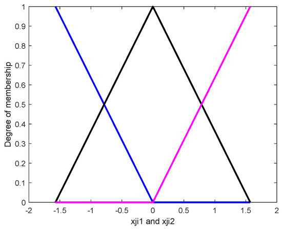
Figure 3. Fuzzy sets.

The communication delays are set as

$$\begin{array}{c}{d}_{m1}=sin\left({\displaystyle \frac{1}{2}}t\right)+1,d_{m2}=sin\left({\displaystyle \frac{1}{5}}t\right)+1\hfill \\ d_{s1}=sin\left({\displaystyle \frac{1}{4}}t\right)+1,d_{s2}=sin\left({\displaystyle \frac{1}{3}}t\right)+1,\mu =0.7\hfill \end{array}$$

The parameters of failures are selected as ${\tilde{m}}_{mib}=0.85$, ${\tilde{m}}_{sib}=0.85(i=1,2)(b=1,2)$, $\mathbb{E}\{{\theta }_{nmi}\left(k\right)=1\}=0.35$, $\mathbb{E}\{{\theta }_{nsi}\left(k\right)=1\}=0.45$, $n=1,2,\cdots ,p$, where

$$\begin{array}{c}\left\{\begin{array}{c}0.75\le m_{nmi}\le 0.85,{\theta }_{nmi}=1\\ 0.85\le m_{nmi}\le 0.95,{\theta }_{nmi}=0\end{array}\right.,\hfill \\ \left\{\begin{array}{c}0.75\le m_{nsi}\le 0.85,{\theta }_{nsi}=1\\ 0.85\le m_{nsi}\le 0.95,{\theta }_{nsi}=0\end{array}\right.\hfill \end{array}$$

Through Theorem 3, the following results are obtained:

$$\begin{array}{cc}\hfill K_{m11}=& \left[\begin{array}{cccc}0.0206& -0.0181& 0.0010& -0.0027\\ -0.0339& 0.0368& 0.0002& 0.0062\end{array}\right],\hfill \\ \hfill K_{m21}=& \left[\begin{array}{cccc}0.0280& -0.0173& -0.0004& -0.0006\\ -0.0480& 0.0389& 0.0016& 0.0037\end{array}\right],\hfill \\ \hfill K_{s11}=& \left[\begin{array}{cccc}0.0344& -0.0285& 0.0020& -0.0043\\ -0.0544& 0.0560& -0.0004& 0.0094\end{array}\right],\hfill \\ \hfill K_{s21}=& \left[\begin{array}{cccc}0.0337& -0.0309& 0.0027& -0.0055\\ -0.0540& 0.0603& -0.0013& 0.0110\end{array}\right],\hfill \\ \hfill K_{m12}=& \left[\begin{array}{cccc}0.0012& -0.0009& 0.0007& 0.0000\\ 0.0001& 0.0043& -0.0008& 0.0002\end{array}\right],\hfill \\ \hfill K_{m22}=& \left[\begin{array}{cccc}0.0017& -0.0013& 0.0001& -0.0006\\ 0.0028& 0.0057& -0.0005& -0.0007\end{array}\right],\hfill \end{array}$$

$$\begin{array}{cc}\hfill K_{s12}=& \left[\begin{array}{cccc}0.0022& -0.0013& 0.0011& 0.0000\\ 0.0003& 0.0072& -0.0012& 0.0004\end{array}\right],\hfill \\ \hfill K_{s22}=& \left[\begin{array}{cccc}0.0018& -0.0016& 0.0017& 0.0004\\ -0.0002& 0.0073& -0.0018& -0.0002\end{array}\right],\hfill \\ \hfill K_{m13}=& \left[\begin{array}{cccc}19.7263& -16.8186& 3.4577& -2.9499\\ -100.8789& 87.0535& -16.7270& 14.3567\end{array}\right],\hfill \\ \hfill K_{m23}=& \left[\begin{array}{cccc}19.6649& -16.7280& 3.4105& -2.9245\\ -101.0030& 87.2124& -16.8201& 14.4125\end{array}\right],\hfill \\ \hfill K_{s13}=& \left[\begin{array}{cccc}19.6173& -16.6109& 3.4252& -2.9185\\ -100.9905& 87.2515& -16.7678& 14.3959\end{array}\right],\hfill \\ \hfill K_{s23}=& \left[\begin{array}{cccc}19.6623& -16.6773& 3.4472& -2.9360\\ -100.8945& 87.1448& -16.8763& 14.4926\end{array}\right],\hfill \\ \hfill K_{m14}=& \left[\begin{array}{cccc}0.0052& -0.0012& 0.0007& -0.0001\\ -0.0052& 0.0093& 0.0001& 0.0015\end{array}\right],\hfill \\ \hfill K_{m24}=& \left[\begin{array}{cccc}0.0076& -0.0007& -0.0015& 0.0005\\ -0.0099& 0.0136& -0.0002& -0.0028\end{array}\right],\hfill \\ \hfill K_{s14}=& \left[\begin{array}{cccc}0.0098& -0.0022& 0.0011& -0.0001\\ -0.0094& 0.0172& 0.0003& 0.0023\end{array}\right],\hfill \\ \hfill K_{s24}=& \left[\begin{array}{cccc}0.0081& -0.0024& 0.0020& -0.0002\\ -0.0077& 0.0144& 0.0006& 0.0039\end{array}\right],\hfill \\ \hfill K_{m15}=& \left[\begin{array}{cccc}0.1468& -0.1382& 0.0042& -0.0081\\ -0.2253& 0.2248& -0.0059& 0.0150\end{array}\right],\hfill \\ \hfill K_{m25}=& \left[\begin{array}{cccc}0.1831& -0.1605& -0.0027& 0.0004\\ -0.2954& 0.2747& 0.0018& -0.0008\end{array}\right],\hfill \\ \hfill K_{s15}=& \left[\begin{array}{cccc}0.2434& -0.2275& 0.0051& -0.0104\\ -0.3675& 0.3670& -0.0065& 0.0191\end{array}\right],\hfill \\ \hfill K_{s25}=& \left[\begin{array}{cccc}0.2262& -0.2155& 0.0074& -0.0107\\ -0.3421& 0.3448& -0.0085& 0.0193\end{array}\right],\hfill \\ \hfill K_{m16}=& \left[\begin{array}{cccc}0.0022& -0.0005& 0.0000& 0.0000\\ -0.0013& 0.0027& 0.0001& 0.0001\end{array}\right],\hfill \\ \hfill K_{m26}=& \left[\begin{array}{cccc}0.0040& 0.0001& -0.0007& 0.0004\\ -0.0036& 0.0053& -0.0007& -0.0011\end{array}\right],\hfill \\ \hfill K_{s16}=& \left[\begin{array}{cccc}0.0041& -0.0009& 0.0000& 0.0000\\ -0.0023& 0.0050& 0.0001& 0.0002\end{array}\right],\hfill \\ \hfill K_{s26}=& \left[\begin{array}{cccc}0.0032& -0.0010& 0.0001& -0.0000\\ -0.0017& 0.0039& 0.0008& 0.0002\end{array}\right],\hfill \\ \hfill K_{m17}=& \left[\begin{array}{cccc}19.6178& -16.9980& -0.1422& 0.1019\\ -126.1310& 110.4224& -1.6427& 1.7055\end{array}\right],\hfill \\ \hfill K_{m27}=& \left[\begin{array}{cccc}19.4410& -16.8080& -0.1425& 0.0881\\ -126.4699& 110.7685& -1.5951& 1.6406\end{array}\right],\hfill \end{array}$$

$$\begin{array}{cc}\hfill K_{s17}=& \left[\begin{array}{cccc}19.6332& -16.9116& -0.1323& 0.0967\\ -126.1837& 110.5798& -1.6380& 1.7060\end{array}\right],\hfill \\ \hfill K_{s27}=& \left[\begin{array}{cccc}19.7837& -17.0679& -0.1058& 0.0749\\ -125.9301& 110.3306& -1.5890& 1.6657\end{array}\right],\hfill \\ \hfill K_{m18}=& \left[\begin{array}{cccc}0.0034& -0.0017& 0.0017& -0.0002\\ -0.0050& 0.0071& -0.0001& 0.0032\end{array}\right],\hfill \\ \hfill K_{m28}=& \left[\begin{array}{cccc}0.0102& -0.0024& 0.0009& -0.0002\\ 0.0063& 0.0183& -0.0002& 0.0016\end{array}\right],\hfill \\ \hfill K_{s18}=& \left[\begin{array}{cccc}0.0074& -0.0038& 0.0037& -0.0005\\ -0.0108& 0.0155& -0.0003& 0.0070\end{array}\right],\hfill \\ \hfill K_{s28}=& \left[\begin{array}{cccc}0.0029& -0.0048& 0.0039& -0.0004\\ -0.0166& 0.0094& 0.0000& 0.0074\end{array}\right],\hfill \\ \hfill K_{m19}=& \left[\begin{array}{cccc}0.0503& -0.0391& 0.0028& -0.0074\\ -0.0825& 0.0779& -0.0008& 0.0160\end{array}\right],\hfill \\ \hfill K_{m29}=& \left[\begin{array}{cccc}0.0586& -0.0354& -0.0008& -0.0015\\ -0.1020& 0.0773& 0.0031& 0.0064\end{array}\right],\hfill \\ \hfill K_{s19}=& \left[\begin{array}{cccc}0.0853& -0.0632& 0.0050& -0.0119\\ -0.1352& 0.1225& -0.0024& 0.0246\end{array}\right],\hfill \\ \hfill K_{s29}=& \left[\begin{array}{cccc}0.0828& -0.0670& 0.0073& -0.0148\\ -0.1327& 0.1292& -0.0049& 0.0281\end{array}\right].\hfill \end{array}$$

In this article, we consider the interactive torque of human operators and environments as the passive spring–damper model, which can be described as

$$\begin{array}{c}\hfill \begin{array}{c}{F}_{hi}=f_{hi}+D_{hi}{\dot{q}}_{mi}+S_{hi}{q}_{mi}\hfill \\ F_{ei}=f_{ei}+D_{ei}{\dot{q}}_{si}+S_{ei}{q}_{si}\hfill \end{array}\end{array}$$

where $D_{hi},D_{ei}\in {\mathcal{R}}^{n\times n}$ denote the damping matrices of the operator and environment. $S_{hi},S_{ei}\in R^{n\times n}$ express the spring matrices of the operator and environment. $f_{hi}$ and $f_{ei}$ are the extra operator and environment torque, and they are assumed to be bounded. $D_{hi}$, $D_{ei}$, $S_{hi}$, $S_{ei}$ are all positive definite and diagonal constant matrices, and $D_{h1}=D_{h2}=diag(0.05,0.05)$, $S_{h1}=diag(3,3)$, $S_{h2}=diag(2.95,2.95)$, $D_{e1}=D_{e2}=diag(0.008,0.008)$, $S_{e1}=diag(0.08,0.08)$, and $S_{e2}=diag(0.06,0.06)$.

The position tracking performance of the corresponding master–slave robots were achieved and are shown in Figure 2. The synchronous motion performance of the slave robots is shown in Figure 3. Obviously, Figure 2 and Figure 3 reflect the good displacement tracking performance of the designed control scheme, and we introduced partial actuator failure fault in the simulation period of 2 to 3 s, with the simulation results showing strong system robustness. The corresponding force feedback tracking performance of environmental force and human force is shown in Figure 4 and Figure 5, respectively. This reflects the good fitting and tracking performance of the controller’s environmental force and operating force. From the above results, it is obvious that the designed controller is effective, even in the case of partial actuator failure. By using the algorithm in reference [4], a comparison example is given in Figure 6, Figure 7 and Figure 8, and the closed loop is uncontrollable when actuator failure exists.

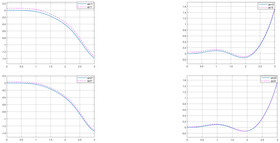
Figure 4. Synchronous motion of master and slave robots by using the proposed fault-tolerant control scheme.

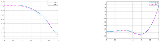
Figure 5. Synchronous motion of Slave 1 and Slave 2 robots.

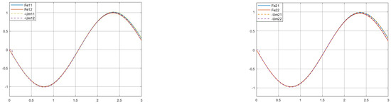
Figure 6. Fitting of environmental force.

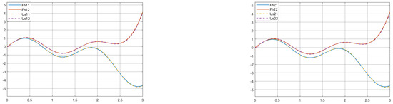
Figure 7. Fitting of human operating force.

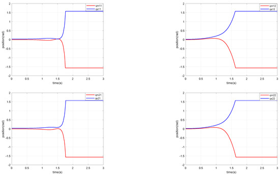
Figure 8. Synchronous motion of master and slave robots by using the algorithm in reference [4].

4. Conclusions

For the considered multilateral teleoperation systems that may have partial actuator failure, the issues of position synchronization and force tracking were achieved simultaneously through a novel failure-distribution-dependent $H_{\infty }$ fuzzy fault-tolerant control scheme. In view of the fact that the multilateral teleoperation systems are nonlinear and have communication delays, the nonlinear multilateral systems are modeled as a kind of T-S fuzzy system with multiple time-varying delays. Then, based on the distribution characteristic of failures, by introducing a series of tradeoff coefficients, a novel failure-distribution-dependent fault-tolerant control algorithm is provided to ensure force tracking in spite of failures, and the purpose of position synchronization is achieved (not only the master and slave robots’ position synchronization but also the position synchronization between each slave robot). After this, the sufficient conditions to ensure the mean square stability and interference suppression level $\gamma$ of the closed-loop system are given. In the end, a numerical example is given to show the effectiveness of the proposed method.

References

- Ye, Y.; Pan, Y.; Hilliard, T. Bilateral teleoperation with time-varying delay: A communication channel passification approach. IEEE/ASME Trans. Mechatronics 2013, 18, 1431–1434. [Google Scholar] [CrossRef]
- Hokayem, P.; Spong, M. Bilateral teleoperation: An historical survey. Automatica 2006, 42, 2035–2057. [Google Scholar] [CrossRef]
- Pan, Y.J.; de Wit, C.C.; Sename, O. A new predictive approach for bilateral teleoperation with applications ot drive-by-wire systems. IEEE Trans. Robot. 2006, 22, 1146–1162. [Google Scholar] [CrossRef]
- Yang, X.; Hua, C.; Yan, J.; Guan, X.P. A new master-slave torque design for teleoperation system by T-S Fuzzy approach. IEEE Trans. Control Syst. Technol. 2015, 23, 1611–1619. [Google Scholar] [CrossRef]
- Yang, Y.; Hua, C.; Li, J.; Guan, X. Finite-time output-feedback synchronization control for bilateral teleoperation system via neural networks. Inf. Sci. 2017, 406–407, 216–233. [Google Scholar] [CrossRef]
- Yang, Y.; Hua, C.; Guan, X. Finite time control design for bilateral teleoperation system with position synchronization error constrained. IEEE Trans. Cybern. 2016, 46, 609–619. [Google Scholar] [CrossRef]
- Wang, H.; Liu, P.X.; Liu, S. Adaptive neural synchronization control for biateral teleoperation systems with time delay and backlash-like hysteresis. IEEE Trans. Cybern. 2017, 47, 3018–3026. [Google Scholar] [CrossRef] [PubMed]
- Sun, D.; Naghdy, F.; Du, H. A novel approach for stability and transparency control of nonlinear bilateral teleoperation system with time delays. Control Eng. Pract. 2016, 47, 15–27. [Google Scholar] [CrossRef]
- Baranitha, R.; Mohajerpoor, R.; Rakkiyappan, R. Bilateral teleoperation of single-master multislave systems with semi-Markovian jump stochastic interval time-varying delayed communication channels. IEEE Trans. Cybern. 2019, 51, 247–257. [Google Scholar] [CrossRef] [PubMed]
- Chen, Z.; Huang, F.; Yang, C.; Yao, B. Adaptive Fuzzy Backstepping Control for Stable Nonlinear Bilateral Teleoperation Manipulators With Enhanced Transparency Performance. IEEE Trans. Ind. Electron. 2020, 67, 746–756. [Google Scholar] [CrossRef]
- Chen, Z.; Pan, Y.J.; Gu, J. A novel adaptive robust control architecture for bilateral teleoperation systems under time-varying delays. Int. J. Robust Nonlinear Control. 2015, 25, 3349–3366. [Google Scholar] [CrossRef]
- Chen, Z.; Pan, Y.J.; Gu, J. Integrated adaptive robust control for multilateral teleoperation systems under arbitrary time delays. Int. J. Robust Nonlinear Control 2016, 26, 2708–2728. [Google Scholar] [CrossRef]
- Li, J.; Liu, X.; Ru, X.; Xu, X. Disturbance rejection adaptive fault-tolerant constrained consensus for multi-agent systems with failures. IEEE Trans. Circuits Syst. II Express Briefs 2020, 67, 3302–3306. [Google Scholar] [CrossRef]
- Li, J.; Ren, W. Finite-horizon H∞ fault-tolerant constrained consensus for multiagent systems with communication delays. IEEE Trans. Cybern. 2019, 51, 416–426. [Google Scholar] [CrossRef]
- Wang, Y.; Song, Y.; Krstic, M.; Wen, C. Fault-tolerant finite time consensus for multiple uncertain nonlinear mechanical systems under single-way directed communication interactions and actuator failures. Automatica 2016, 63, 374–383. [Google Scholar] [CrossRef]
- Li, J.; Xu, Y.; Gu, K.; Li, L.; Xu, X. Mixed passive/H∞ hybrid control for delayed Markovian jump system with actuator constraints and fault alarm. Int. J. Robust Nonlinear Control 2018, 28, 6016–6037. [Google Scholar] [CrossRef]
- Li, J.; Pan, Y.; Su, H.; Wen, C. Stochastic reliable control of a class of networked control systems with actuator faults and input saturation. Int. J. Control Autom. Syst. 2014, 12, 564–571. [Google Scholar] [CrossRef]
- Qiu, J.; Wei, Y.; Karimi, H.R.; Gao, H. Reliable control of discrete-time piecewise-affine time-delay systems via output feedback. IEEE Trans. Reliab. 2018, 67, 79–91. [Google Scholar] [CrossRef]
- Dong, S.; Wu, Z.; Shi, P.; Su, H.; Lu, R. Reliable control of fuzzy systems with quantization and switched actuator failures. IEEE Trans. Syst. Man Cybern. Syst. 2017, 47, 2198–2208. [Google Scholar] [CrossRef]
- Li, X.; Yang, G.H. Neural-network-based adaptive decentralized fault-tolerant control for a class of interconnected nonlinear systems. IEEE Trans. Neural Netw. Learn. Syst. 2018, 29, 144–155. [Google Scholar] [CrossRef]
- He, X.; Wang, Z.; Qin, L.; Zhou, D. Active fault-tolerant control for an Internet-based networked three-tank system. IEEE Trans. Control Syst. Technol. 2016, 24, 2150–2157. [Google Scholar] [CrossRef]
- Shen, Q.; Yue, C.; Goh, C.H.; Wang, D. Active fault-tolerant control system design for spacecraft attitude maneuvers with actuator saturation and faults. IEEE Trans. Ind. Electron. 2019, 66, 3763–3772. [Google Scholar] [CrossRef]
- Lan, J.; Patton, R.J. A new strategy for integration of fault estimation within fault-tolerant control. Automatica 2016, 69, 48–59. [Google Scholar] [CrossRef]
- Ma, H.; Yang, G. Adaptive fault tolerant control of cooperative heterogeneous system with actuator faults and unreliable interconnections. IEEE Trans. Autom. Control 2016, 61, 3240–3255. [Google Scholar] [CrossRef]
- Rakkiyappan, R.; Baranitha, R.; Zeng, Z. Hidden Markov-Model-Based Control Design for Multilateral Teleoperation System With Asymmetric Time-Varying Delays. IEEE Trans. Syst. Man Cybern. Syst. 2022, 52, 1958–1969. [Google Scholar] [CrossRef]
- Yang, Q.; Ma, X.; Wang, W.; Peng, D. Adaptive Non-Singular Fast Terminal Sliding Mode Trajectory Tracking Control for Robot. Manipulators. Electronics 2022, 11, 3672. [Google Scholar] [CrossRef]
- Li, J.; Wang, A.; Miao, K.; Li, L.S. Failure-distribution-dependent H∞ fuzzy fault-tolerant control for multiple-degree-of-freedom nonlinear bilateral teleoperation system. J. Frankl. Inst. 2020, 357, 13511–13533. [Google Scholar] [CrossRef]
- Tseng, C.S.; Chen, B.S.; Uang, H.J. Fuzzy tracking control design for nonlinear dynamic systems via T-S fuzzy model. IEEE Trans. Fuzzy Syst. 2001, 9, 381–392. [Google Scholar] [CrossRef]
- Li, H.; Liu, H.; Gao, H.; Shi, P. Reliable fuzzy control for active suspension systems with actuator delay and fault. IEEE Trans. Fuzzy Syst. 2012, 20, 342–357. [Google Scholar] [CrossRef]
- Sun, D. Passivity Control of Bilateral and Multilateral Teleoperation Systems. Ph.D. Dissertation, School of Electrical, Computer & Telecommunication Engineering, University of Wollongong, Wollongong, NSW, Australia, 2015. [Google Scholar]
- Gu, K.; Chen, J.; Kharitonov, V.L. Stability of Time-Delay Systems; Springer Science and Business Media: Berlin/Heidelberg, Germany, 2003. [Google Scholar]
- Xie, L. Output feedback H∞ control of systems with parameter uncertainty. Int. J. Control 1996, 64, 570–741. [Google Scholar] [CrossRef]
- Horn, R.A.; Johnson, C.R. Matrix Analysis; Cambridge University Press: New York, NY, USA, 1987. [Google Scholar]
Disclaimer/Publisher’s Note: The statements, opinions and data contained in all publications are solely those of the individual author(s) and contributor(s) and not of MDPI and/or the editor(s). MDPI and/or the editor(s) disclaim responsibility for any injury to people or property resulting from any ideas, methods, instructions or products referred to in the content. |
© 2024 by the authors. Licensee MDPI, Basel, Switzerland. This article is an open access article distributed under the terms and conditions of the Creative Commons Attribution (CC BY) license (https://creativecommons.org/licenses/by/4.0/).