Figure 1.
Data volume and the rise in DCN energy consumption: The projected exponential growth in global data volume from 2010 to 2025, measured in zettabytes, is illustrated. This surge in data processing significantly loads DCNs, which are reported to consume roughly of global energy according to the Natural Resources Defense Council.
Figure 2.
Flow of control of FPLF: FPLF operates in a sequential manner. The output from each of three stages feeds into the next.
Figure 2.
Flow of control of FPLF: FPLF operates in a sequential manner. The output from each of three stages feeds into the next.
Figure 3.
The pure consolidation method and the RTP-aware consolidation method of power optimization subject to an RTP-flow delay constraint are illustrated. In sub-figure (
a): [
![Electronics 13 02976 i001]()
]: Represents the consolidation of three flows. [
![Electronics 13 02976 i002]()
]: Represents the consolidation of 4 flows on segment path
from different sources. [
![Electronics 13 02976 i003]()
]: Signifies the sum of 2 flows. In sub-figure (
b): [
![Electronics 13 02976 i001]()
]: Represents the consolidation of (two plus the RTP flow). [
![Electronics 13 02976 i002]()
]: Represents the consolidation of 3 flows because the RTP flow was moved to an alternative path, represented by [
![Electronics 13 02976 i001]()
].
Figure 4.
The Q-PoPS framework for power-optimized QoS for SD-DCNs is illustrated. It leverages the northbound (POX) and the southbound (OpenFlow) interfaces. The core innovation lies in Q-PoPS, which integrates information from the Classifier, Monitoring, and FPLF components to manage power and QoS for real-time traffic, which is represented by
.
Section 5.5 details the operation of Q-PoPS.
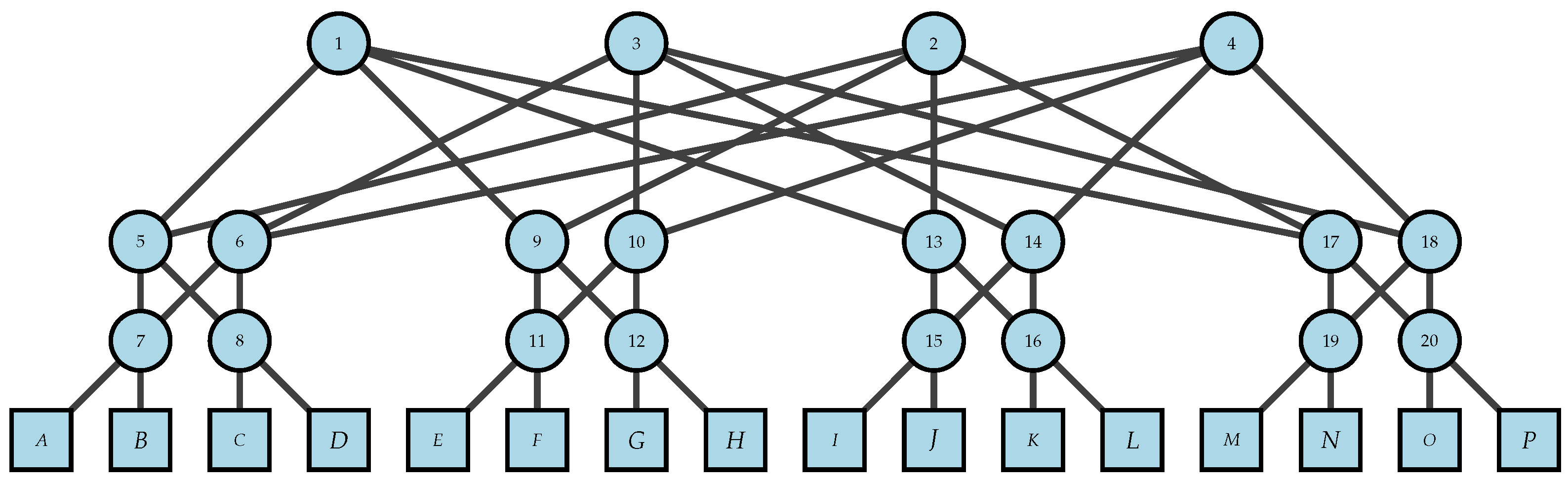
Figure 5.
Emulated fat-tree topology. The figure illustrates a fat-tree network where k represents the parameter that defines the number of switches and connections in the network. Specifically, indicates a topology with four levels of switches and a total of switches in the network. This topology is often used in data center networks to provide scalable and fault-tolerant network structures.
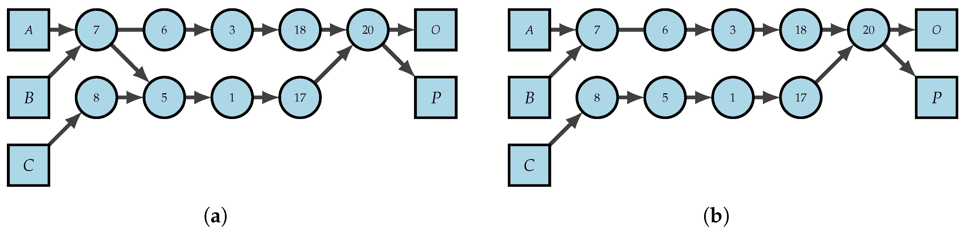
Figure 6.
Illustration of the active subset of the network graph, G, before (LHS window) and after (RHS window) a delay event triggered by congested real-time traffic. (a) Q-PoPS: active subset of the graph, G, before the delay event. (b) Q-PoPS, active subset of the graph, G, after the delay event.
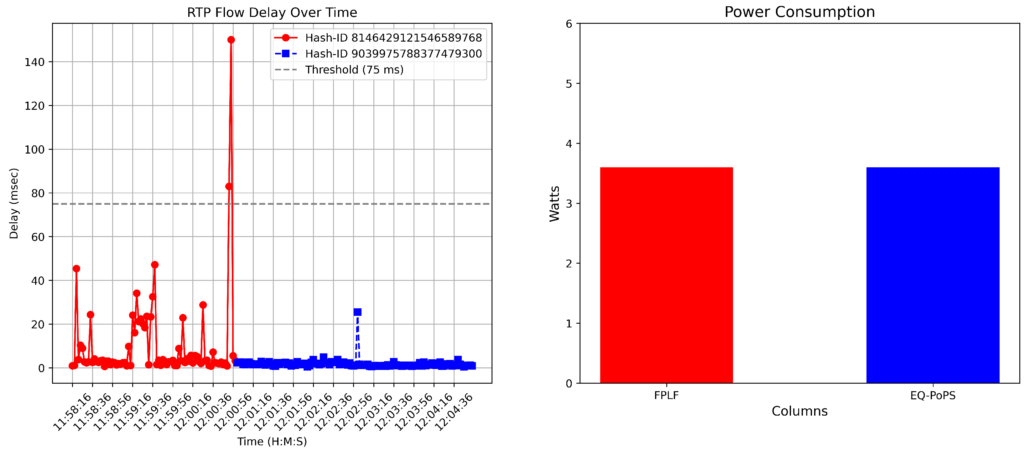
Figure 7.
Comparison of power consumption, using the pure FPLF algorithm proposed in [
10], and the Q-PoPS method (RHS window), along with delay value of the RTP Flow before and after the delay event (LHS window).
Figure 7.
Comparison of power consumption, using the pure FPLF algorithm proposed in [
10], and the Q-PoPS method (RHS window), along with delay value of the RTP Flow before and after the delay event (LHS window).
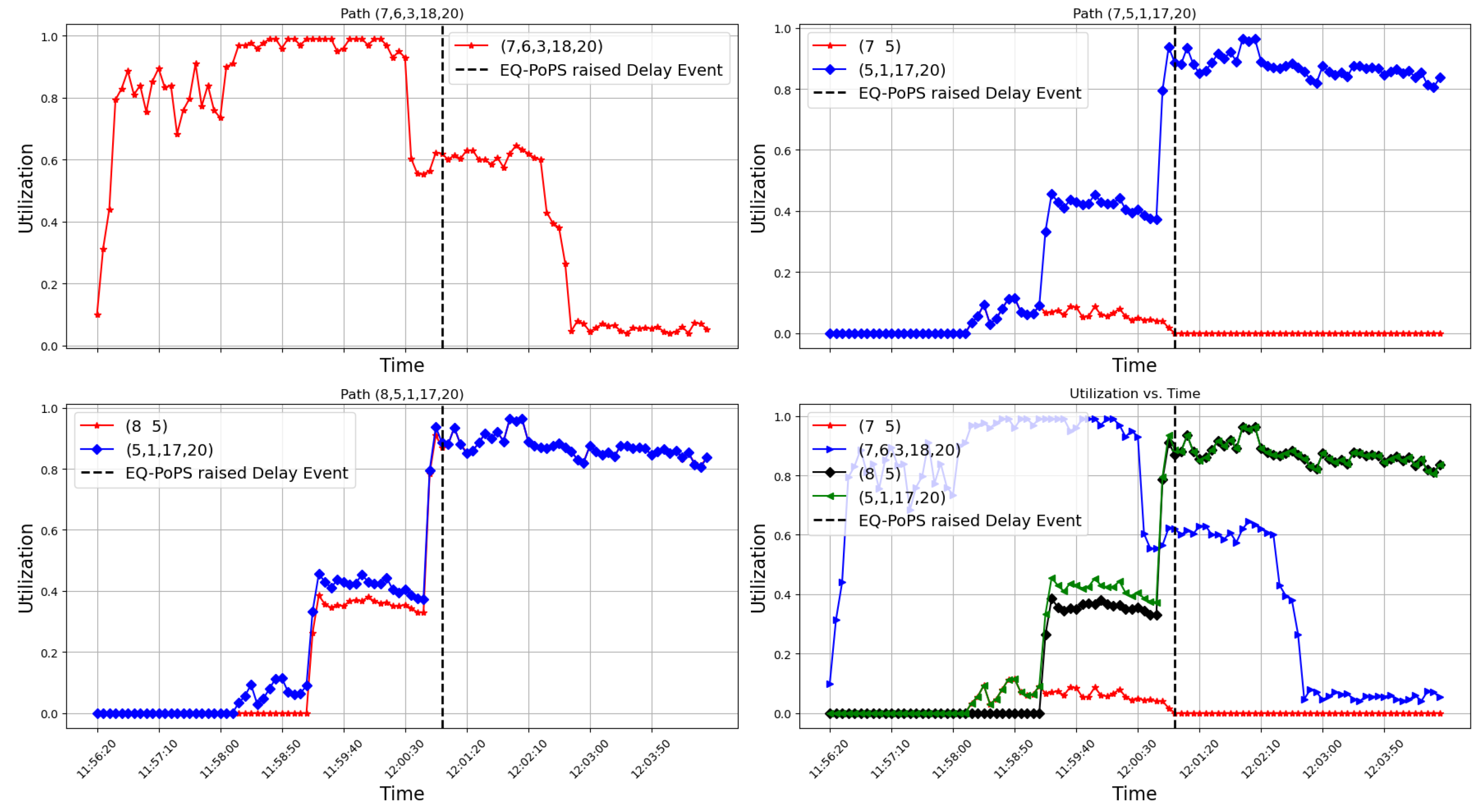
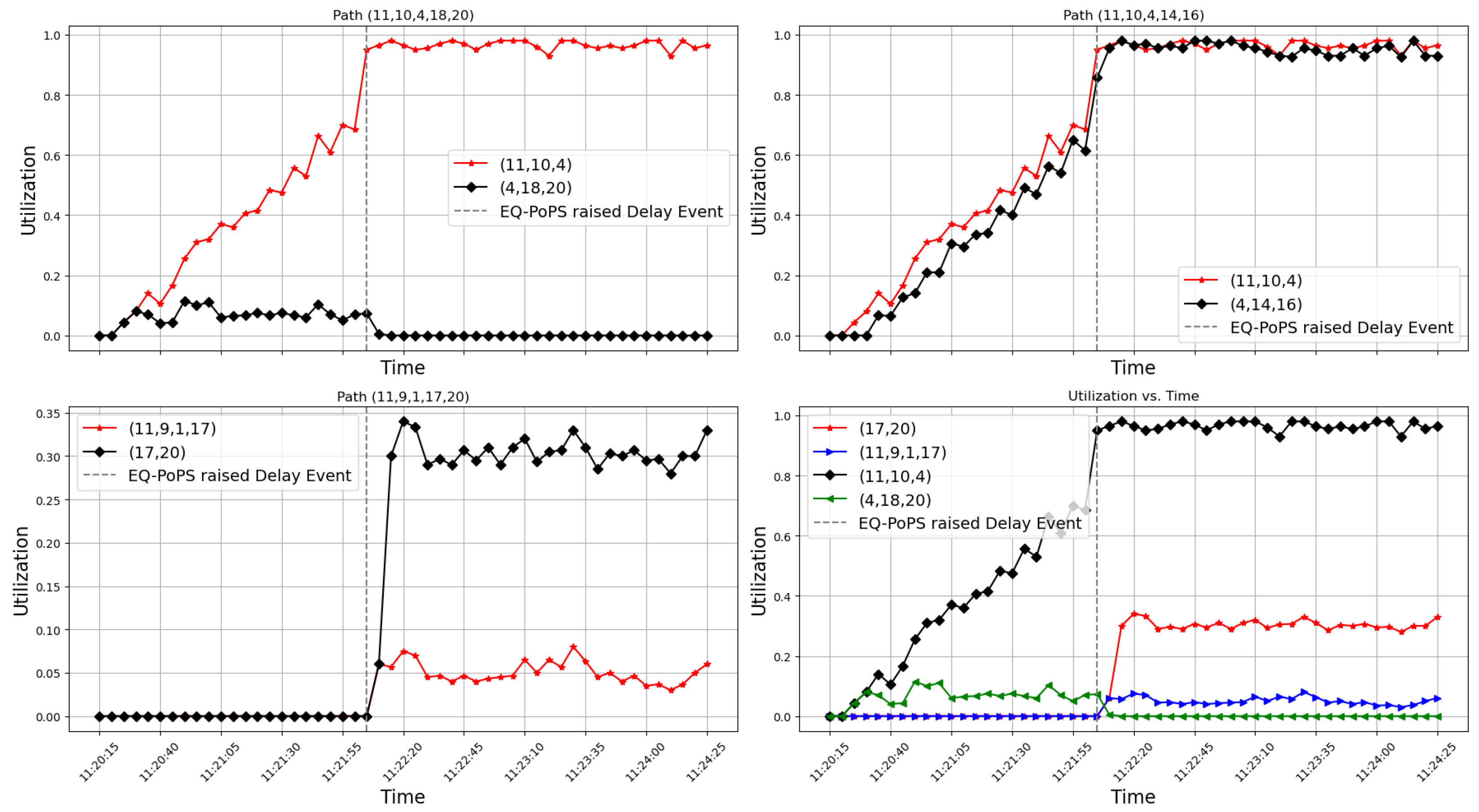
Figure 8.
Visualization of the active link path utilization as a function of simulation time. The upper LHS window displays the utilization for the path , where all the links in the path have the same utilization. In the upper RHS window, the path is shown, where all links have the same utilization except for link, , because it is not a shared link. The utilization of path is presented in the lower LHS window. The lower RHS window displays all the critical links that Q-PoPS relied on to make decisions about alternative paths.
Figure 9.
We illustrate how Q-PoPS optimizes power consumption for the midrange traffic scenario by showing the state of the graph, G, before and after the delay event. (a) Q-PoPS: active subset of graph, G, before the delay event. (b) Q-PoPS: active subset of graph, G, after the delay event.
Figure 9.
We illustrate how Q-PoPS optimizes power consumption for the midrange traffic scenario by showing the state of the graph, G, before and after the delay event. (a) Q-PoPS: active subset of graph, G, before the delay event. (b) Q-PoPS: active subset of graph, G, after the delay event.
Figure 10.
We compare the power consumption of SD-DCNs managed by FPLF and Q-PoPS. FPLF exhibits lower power usage (4 Watts). Q-PoPS consumes a larger power consumption ( Watts). Q-PoPS dynamically reroutes the real-time traffic flow when congestion occurs, requiring the activation of additional ports, 4 in this case. The primary result communicated is the trade-off between power efficiency and real-time traffic management.
Figure 11.
Visualization of active link path utilization as a function of simulation time. The upper LHS window shows the link utilization of the path as time evolves. The upper RHS second displays the path link utilization for the path . The path segment is utilized more because it supports both ICMP and RTP traffic before the delay event. Conversely, the link path carries only ICMP throughout the simulation. The lower LHS window presents the utilization of the link path . The lower RHS window showcases all the critical links that Q-PoPS relies on for decision-making regarding alternative paths.
Figure 12.
Q-PoPS optimizes delay in the worst-case scenario; however, due to a limited active subset (a), Q-PoPS finds a completely new path (b) to meet real-time traffic needs. (a) Q-PoPS: active subset of graph G before the delay event. (b) Q-PoPS: active subset of a graph, G, after the delay event.
Figure 13.
Comparison of power consumption between FPLF and Q-PoPS (RHS window), along with delay value for the RTP Flow before and after a delay event (LHS window), worst-case solution.
Figure 13.
Comparison of power consumption between FPLF and Q-PoPS (RHS window), along with delay value for the RTP Flow before and after a delay event (LHS window), worst-case solution.
Figure 14.
Visualization of paths utilization during the simulation. The path shared both ICMP and RTP traffic until 17:04:00, then it started carrying ICMP traffic only for the remaining simulation time, while the path served as the alternative path for transmitting the RTP flow.
Figure 14.
Visualization of paths utilization during the simulation. The path shared both ICMP and RTP traffic until 17:04:00, then it started carrying ICMP traffic only for the remaining simulation time, while the path served as the alternative path for transmitting the RTP flow.
Table 1.
Conventional names of parameters used in problem formulation.
Table 1.
Conventional names of parameters used in problem formulation.
| Parameters | Definitions |
|---|
| | Delay on link in ms. |
| | Flow delay, where the set of flow delays is , and . |
| | Identifies the flow based on the 3-tuple (transport layer,
network layer, link layer), where , where the set
of all flow ids is . |
| | Is the set of all flows. A flow consists of ths terms,
. The source is denoted . The flow destination
is denoted, . Its bit rate is denoted
. The flow ID is , and the flow delay is . |
| | The set of energy-efficient shortest paths is denoted
, where a path,
is represented by a set of switches between the servers of DCNs, where . |
| | The set of RTP flows is denoted as , where . |
| | Positive-valued variable,, represents the traffic
volume over the link . |
| Constant | Definitions |
| | Time delay threshold value. |
| | Bandwidth of link . |
| | |
| Decision Variable | Definitions |
| | |
| | |
Table 2.
Characteristics of the traffic used in the SD-DCN as outlined in [
1].
Table 2.
Characteristics of the traffic used in the SD-DCN as outlined in [
1].
| Characteristics | Type of Distribution | Shape () | Scale () |
|---|
| OFF periods | Weibull | 10 | 100 |
| ON periods | Pareto | 10 | 100 |
Table 3.
Flow delay analysis: We present a sample of the Q-PoPS flow delay analysis, focusing on monitoring traffic and its impact on delay, particularly for Real-time Transport Protocol (RTP) flows.
Table 3.
Flow delay analysis: We present a sample of the Q-PoPS flow delay analysis, focusing on monitoring traffic and its impact on delay, particularly for Real-time Transport Protocol (RTP) flows.
| Index | Time | | Flow Type | Flow Src and Dst | Path | Delay |
|---|
| 1 | 17:10:20 | 4.94 × 10¹⁸ | RTP | E P | 11 9 2 17 20 | 1.703501 |
| 2 | 17:10:29 | −1.24 × 10¹⁸ | RTP | A D | 7 5 8 | 1.057863 |
| 3 | 17:10:38 | 5.18 × 10¹⁸ | ICMP | F L | 11 9 2 13 16 | not applied |
| 4 | 17:10:42 | 5.84 × 10¹⁸ | ICMP | F L | 11 9 2 13 16 | not applied |
| 5 | 17:10:48 | −6.55 × 10¹⁸ | ICMP | F L | 11 9 2 13 16 | not applied |
| 6 | 17:10:58 | 1.57 × 10¹⁸ | ICMP | F L | 11 9 2 13 16 | not applied |
| 7 | 17:11:08 | −1.82 × 10¹⁸ | ICMP | F L | 11 9 2 13 16 | not applied |
| 8 | 17:11:18 | −1.59 × 10¹⁷ | ICMP | F L | 11 9 2 13 16 | not applied |
| 9 | 17:11:28 | −4.68 × 10¹⁸ | ICMP | F L | 11 9 2 13 16 | not applied |
| 10 | 17:11:38 | −3.00 × 10¹⁸ | ICMP | F L | 11 9 2 13 16 | not applied |
| 11 | 17:11:48 | −1.21 × 10¹⁸ | ICMP | F L | 11 9 2 13 16 | not applied |
| 12 | 17:11:58 | 6.60 × 10¹⁸ | ICMP | F L | 11 9 2 13 16 | not applied |
| 13 | 18:12:08 | 4.94 × 10¹⁸ | RTP | E P | 11 9 2 17 20 | 161.152601 |
| 14 | 19:12:08 | −1.24 × 10¹⁸ | RTP | A D | 11 9 2 17 20 | 1.467466 |
Table 4.
Paths and saturation states as a function of simulation time: The state of paths during periods of saturation and their impact on delay is described.
Table 4.
Paths and saturation states as a function of simulation time: The state of paths during periods of saturation and their impact on delay is described.
| Start Time | Path | Number of Flows | Saturated Period (s) | Start/End of Saturated Period | Delay of Saturated Period |
|---|
| 11:56:20 | | multiple ICMP | 120 | 11:58:30 to 12:00:30 | not applied |
| 11:58:20 | | single RTP | 60 | 12:01:00 to 12:02:00 | delay |
| 11:59:10 | | multiple ICMP | 60 | 12:01:00 to 12:02:00 | not applied |
| 12:01:00 | | multiple ICMP/single RTP | none | none | delay |
Table 5.
Paths and saturation states as a function of simulation time: In response to congestion changes as time evolves, Q-PoPS finds alternative paths.
Table 5.
Paths and saturation states as a function of simulation time: In response to congestion changes as time evolves, Q-PoPS finds alternative paths.
| Start Time | Path | Number of Flows | Saturated Period (s) | Start/End of Saturated Period | Delay of Saturated Period |
|---|
| 11:20:00 | | single RTP | 120 | 11:22:05 to 11:24:25 | delay |
| 11:20:10 | | multiple ICMP | 120 | 11:22:05 to 11:24:25 | not applied |
| 11:22:20 | | single RTP | none | none | delay |
| 11:22:20 | | multiple ICMP | none | none | not applied |
Table 6.
Path states in the worst case scenario simulation as a function of simulation time.
Table 6.
Path states in the worst case scenario simulation as a function of simulation time.
| Start Time | Path | Number of Flows | Saturated Period (s) | Start/End of Saturated Period | Delay of Saturated Period |
|---|
| 17:01:11 | | single RTP/multiple ICMP | 140 | 11:04:20 to 11:06:20 | delay |
| 17:04:01 | | single RTP | none | none | delay |


 ]: Represents the consolidation of three flows. [
 ]: Represents the consolidation of 4 flows on segment path from different sources. [
 ]: Signifies the sum of 2 flows. In sub-figure (b): [


