Article

Enhanced Text Classification with Label-Aware Graph Convolutional Networks

1
Department of Information Engineering and Computer Science, Feng Chia University, Taichung 407, Taiwan
2
Department of Information Management, Chaoyang University of Technology, Taichung 413, Taiwan
*
Author to whom correspondence should be addressed.
Electronics 2024, 13(15), 2944; https://doi.org/10.3390/electronics13152944
Submission received: 30 June 2024 / Revised: 18 July 2024 / Accepted: 25 July 2024 / Published: 25 July 2024

Abstract

:
Text classification is an important research field in text mining and natural language processing, gaining momentum with the growth of social networks. Despite the accuracy advancements made by deep learning models, existing graph neural network-based methods often overlook the implicit class information within texts. To address this gap, we propose a graph neural network model named LaGCN to improve classification accuracy. LaGCN utilizes the latent class information in texts, treating it as explicit class labels. It refines the graph convolution process by adding label-aware nodes to capture document–word, word–word, and word–class correlations for text classification. Comparing LaGCN with leading-edge models like HDGCN and BERT, our experiments on Ohsumed, Movie Review, 20 Newsgroups, and R8 datasets demonstrate its superiority. LaGCN outperformed existing methods, showing average accuracy improvements of 19.47%, 10%, 4.67%, and 0.4%, respectively. This advancement underscores the importance of integrating class information into graph neural networks, setting a new benchmark for text classification tasks.

1. Introduction

Text classification stands as a cornerstone task in natural language processing, aiming to algorithmically ascertain the class of a given document by analyzing its content. Traditional approaches have largely centered on feature computation to bolster classification efficacy, employing techniques such as Bag-of-Words (BoW) and Term Frequency-Inverse Document Frequency (TF-IDF). In contrast, deep learning methodologies, such as Convolutional Neural Networks (CNNs) [1] and Recurrent Neural Networks (RNNs), learn representations that capture contextual information to enhance classification. Notably, the Bidirectional Encoder Representations from Transformers (BERT) model [2] has shown its capability in considering the contextual information within documents comprehensively. However, due to their inability to utilize content information from similar documents in the same class, these methods may be constrained, potentially decreasing their classification accuracy. Graph Neural Networks (GNNs), with their capacity to incorporate the content of neighboring documents through graph convolution operations, present a promising solution to this limitation [3,4,5].
Recently, there has been a significant increase in exploring the application of graph neural networks for text classification. TextGCN [6] innovates by constructing a heterogeneous graph that includes both document and word nodes, effectively recasting text classification as a node classification problem. Text Level GNN [7] extends this paradigm by transforming node classification into graph classification, utilizing a global graph to access a more extensive corpus of textual information. TextING [8] takes a tailored approach by constructing individual graphs for each document, thereby enhancing the model’s generalization capabilities. TensorGCN [9] goes a step further by creating multiple word–word relation graphs, tapping into an even broader spectrum of textual data. Additionally, HDGCN [10], drawing on the principles of ChebNet, integrates an attention mechanism to refine graph updates and mitigate the issue of over-smoothing.
Despite recent advancements in text classification, a common oversight persists: the omission of class information for words within the text. This class information, referred to as the “label” of a word, is crucial for models to infer document classes from nuanced textual details. For example, consider a sample sentence “this athlete’s performance on the field is impressive”, from a news article classified under the SPORT category. The word “athlete” itself is more informative for the SPORT category than the POLITICS category. That is, the label of “athlete” for news text classification is SPORT. As another example, consider the sentence “this music performance is impressive” from a short text message classified as POSITIVE sentiment. The word ‘impressive’ itself is more informative for the POSITIVE class than the NEGATIVE class. In other words, the label of “impressive” for sentiment classification is POSITIVE.
Additionally, we can infer the class of a document by jointly referencing the “class” proportions of different words in the text. For instance, in the previously mentioned example “this music performance is impressive”, we have neutral words like “this”, “performance”, and “is”, where the positive-to-negative category ratio for these words is approximately 5:5. However, for the word “impressive”, the positive-to-negative ratio is 8:2. This key information determines that this text falls under the positive category. We found that previous literature did not incorporate word “class” information, leading past models to infer document classes merely based on the words contained within the document. They could not accurately infer the class of the document by jointly referencing the “class” proportions of all the words in the document.
By utilizing these word labels, graph neural networks can leverage this class information to potentially improve text classification accuracy. Specifically, awareness of the class associations of words could help graph neural networks better infer document classes from textual semantics. More research is needed to develop methods to effectively incorporate word labels into graph neural network models for text classification.
To address the lack of explicit label information in text classification, we propose the LaGCN (Label-aware Graph Convolutional Network) algorithm. LaGCN innovatively constructs a word–class graph to integrate class labels of words, thereby enriching the text classification process with this information. Experiments demonstrate the benefits of modeling word–class labels, with LaGCN achieving an average accuracy of 93.6% on well-known public datasets. This high accuracy highlights the value of equipping graph neural networks with an awareness of the class associations of words for text classification.
The key contributions of our work are as follows:
  • Introduction of label-aware nodes. We introduce label-aware nodes in the graph convolutional network to explicitly incorporate class information into the model, thereby enhancing the accuracy of text classification.
  • Enhanced graph convolution process. We refine the graph convolution process by capturing document–word, word–word, and word–class correlations through the integration of label-aware nodes.
  • Comprehensive evaluation. We conduct extensive experiments on public datasets (Ohsumed, Movie Review, 20 Newsgroups, and R8) to demonstrate the superiority of LaGCN over existing state-of-the-art models like HDGCN and BERT. Our results show significant accuracy improvements of 19.47%, 10%, 4.67%, and 0.4%, respectively.
  • Setting a new benchmark. Our study highlights the importance of integrating class information into graph neural networks, establishing a new benchmark for text classification tasks.

2. Related Work

Traditional text classification methods, such as Bag-of-Words (BOW) and Term Frequency-Inverse Document Frequency (TF-IDF), have mainly focused on word features [11,12,13,14]. BOW assesses the presence of words within an article, while TF-IDF computes the representation of a document based on word and document frequencies. Word2vec [12] employs the Continuous Bag of Words and Skip-gram models to learn word-level representations that encapsulate contextual information. GloVe [13] and fastText [11] also applied similar techniques for training. Despite their reasonable performance in text classification, these methods fall short in dealing with the complex document semantics.
Deep learning approaches to text classification, including Recurrent Neural Networks (RNNs) and Convolutional Neural Networks (CNNs) [1], have been developed to address these complexities. RNNs process sentences as sequences, utilizing memory cells to preserve sequential information. While they effectively capture contextual information, their dependence on previous state information makes the training and inference processes lengthy. Conversely, CNNs apply filters to capture contextual information more efficiently, avoiding the time-related limitations common in RNNs. However, both RNNs and CNNs encounter challenges in managing long-distance dependencies between words, risking information loss. BERT [2] leverages Self-Attention and Positional Encoding to mitigate these long-distance issues. However, BERT models require significant resources for training and inference, making them less accessible for applications with limited computational power.
Many studies have explored the application of Graph Neural Networks (GNNs) in text classification [15,16,17,18,19]. The primary strength of GNNs lies in their ability to form graph structures and learn the relationships among nodes within the graph. By delineating well-structured graphs with defined nodes and edge weights, GNNs facilitate the derivation of meaningful representations through message propagation [20]. Some well-known GNN methods for text classification are briefly reviewed below.
TextGCN [6] introduces a heterogeneous graph comprising document and word nodes, utilizing TF-IDF values as edge weights between document and word nodes, and Positive Pointwise Mutual Information (PPMI) values between word nodes. Graph convolutional networks enable the transmission of information across nodes, allowing for cross-referencing between not only words but also documents. Nonetheless, it may suffer from scalability issues when dealing with very large datasets of complex graph structure.
Text Level GNN [7] employs both local and global graphs, depicting documents as local graphs while drawing on a global graph for additional textual information. This dual-graph structure aids in referencing document content and external text sources for classification. Still, managing multiple graphs and integrating global context can increase computational complexity and require significant resources.
TextING [8] generates a distinct graph for each document, integrating an attention mechanism to prioritize key information within the graph. This method not only enhances the model’s generalization capacity but also refines classification precision by focusing on essential details. The limitation is that generating separate graphs for each document can be computationally intensive and may not scale well to very large datasets.
TensorGCN [9] constructs a network with varied edge relationships among text nodes, encompassing semantic, syntactic, and contextual links. By combining different perspectives, it offers a more complete consideration of the complex relationships between words, thereby enriching textual representations. Nevertheless, the complexity of handling multiple types of relationships can lead to increased computational demands and difficulties in model optimization.
Lastly, HDGCN [10] manages the information propagation in GCN models by controlling the volume of transmitted information during node transfers. This strategy effectively addresses the over-smoothing problem inherent in GCNs. However, the control adds an additional layer of complexity to the model, potentially increasing computational overhead. Table 1 summarizes the key features and limitations of recent GCN models.

3. Proposed Model

Figure 1 depicts the overall architecture of the proposed LaGCN model, which consists of the following. (1) Text-to-Graph: Constructing the document–word graph ( G d w ), the word–word graph ( G w w ), and the word–class graph ( G w c ) using all the documents. The three graphs will be merged into a heterogeneous graph ( G A ) of the three types of nodes (document, word, and class nodes). (2) Convolution computation: Applying graph convolution by using G A and the embedding matrix (X) of the document, word, and class embedding to aggregate information from the connected nodes. (3) Training and inference: Concurrent training for three distinct tasks, text classification to classify document nodes ( y d i ), word–class prediction to predict class associations of word nodes ( y w j ), and class prediction on class nodes ( y c k ). Note that ‘class node’ and ‘label-aware node’ are used interchangeably in the following context. The overall objective is to optimize document classification with the defined loss functions.

3.1. Text-to-Graph

First, we construct the document–word graph G d w . Given a set of documents D = { d 1 , d 2 , d D } , and the set of distinct words W = { w 1 ,   w 2 ,   w W }     i n   D , let document d i     b e     [ w 1 ,   w 2 , , w s ] , where w j   1 j s is the j-th word appearing in d i . Here, w 1 ,   w 2 , , w s represents the sequence of words in d i , and the order of words is important, as it captures the context within the document. This sequence is treated as a vector of words with a defined order. In the document–word graph G d w ,   an edge e d i ,   w j exists between d i and w j , with edge weight (TF-IDF) t f i j × i d f j . Here, t f i j = c o u n t d i ( w j ) | d i | , where c o u n t d i ( w j ) is the number of w j appearing in d i , and   | d i | is the length of di; i d f j = log | D | | d i     D   a n d   w j     d i | . The adjacency matrix of Gdw is represented by A d w R D × | W | . Such a design (using TF-IDF) allows the model to learn the relationship between words and documents after the following graph convolution. If certain words are used frequently in a document, the document node will have stronger information about these words, and thus, the document can be closer to these words in the vector space.
Figure 1. Overview of Label-Aware Graph Convolutional Network (LaGCN).
Electronics 13 02944 g001
Next, we construct the word–word graph G w w containing all the word nodes. We use a window of length L, and slide the words in document di. Given document d i = [ w 1 ,   w 2 , , w s ] , the sliding produces |s| − L + 1 text-windows, i.e., tw1 = [w1, w2, …, wL], tw2 = [w2, w3, …, wL+1], …, tw|s|−L+1 = [w|s|−L+1, w|s|−L+2, …, ws] . The sliding will be operated with respect to all the documents. Let Nw be the total number of text-windows. We calculate the total number of text-windows having wi, denoted as Nw(wi), and the total number of text-windows having the co-occurrence of wi and wj, denoted as Nw(wi, wj). A co-occurrence of wi and wj is represented as an edge e(wi, wj) in the word–word graph Gww. The edge weight of e(wi, wj) is the Positive Pointwise Mutual Information (PMI) between wi and wj, P M I w i , w j = log p ( w i , w j ) p ( w i ) p ( w j ) , where p w i = N W w i N W and p w i , w j = N W w i , w j N W . The adjacency matrix of Gww is represented by A w w R W × | W | . Such a design allows the model to learn the relationships among words after the graph convolution. If certain words co-occur frequently, the word nodes can be closer in the vector space. Thus, the model may learn relationships from the whole set of documents rather than from a single document.
Last, we build the word–class graph Gwc containing all the word nodes and the class nodes in the text classification tasks. The set of classes C = {Ck1, Ck2, …, C|C|}. Given document d i = [ w 1 ,   w 2 , , w s ] and its class Ck, we will have edges e(w1, Ck), e(w2, Ck), …, e(ws, Ck). Note that if word wj appears in both document di1 of class Ck1 and document di2 of class Ck2, and Ck1 is different from Ck2, then node wj will connect to the two class nodes Ck1 and Ck2 (via two edges). The edge weight of e(wj, ck), the edge between word wj and class ck, is described by the Term Frequency-Inverse Class Frequency (TF-ICF) t f k j × i c f j . Here, t f k j = c o u n t c k ( w j ) | c k | , where c o u n t c k ( w j ) is the number of w j appearing in c k , and   | c k | is the total number of word occurrences in ci; i c f j = log | C | | c k     C   a n d   w j     c k | . The adjacency matrix of Gwc is represented by A w c R W × | C | .
By merging the document–word, word–word, and word–class graphs, we construct an integrated graph GA that connects nodes of documents, words, and classes based on their associations. GA contains three types of nodes and three types of edges; the convolution of the graph allows aggregating relevant information from each node type for enhanced document classification. The merging is as follows. Both Gdw and Gww have word nodes, the nodes representing the same word are merged, i.e., G d w G w w . Then, G w c also has word nodes, and the nodes representing the same word in G d w G w w   are merged. The edge weights are kept intact. The final graph is GA.
GA has three types of nodes, and we may use a matrix of D × W × C × D × W × C to represent the adjacent information, denoted as Adwc. Adwc can be written as A d d A d w A d c A w d A w w A w c A c d A c w A c c . Add and Acc are zero matrices, since no connections exist between documents nor between classes. Adc and Acd are set to the zero matrix, since we should not build or reveal the connections between documents and classes. Therefore, A d w c = 0 A d w 0 A w d A w w A w c 0 A c w 0 , where A d w c R D + W + C × D + W + C , A d w = A w d , A w c = A c w , and ‘ 0 is a zero matrix. Adwc can facilitate the graph convolution process in Section 3.2.

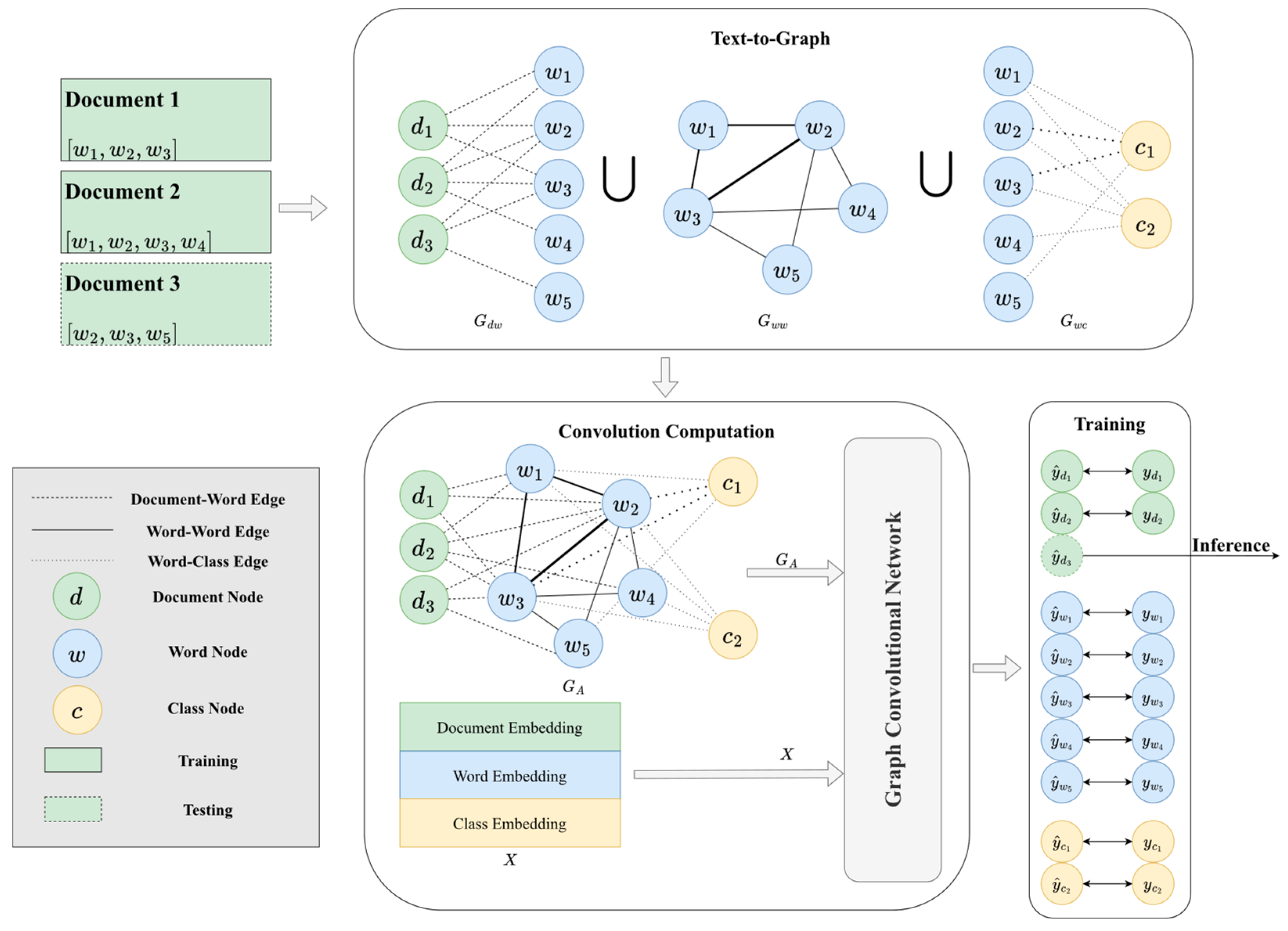
3.2. Convolution Computation

We apply GCN to the constructed heterogeneous graph to integrate relevant signals from the document, word, and class nodes. Given a graph G = ( V ,   E ) with adjacency matrix A , where A i j represent the edge weight between nodes i and j, graph convolution combines node features H l based graph structure; H l + 1 = A ~ H l W l , where A ~ = D 1 2 A D 1 2 is the normalized adjacency matrix, with D as the diagonal node degree matrix of A ( D i i = Σ j A i j ), and W l denotes the trainable weight matrix for layer l . Let the embedding dimension be d. Two GCN layers are implemented here. In the first layer, we propagate node features X by H 1 = R E L U ( A ~ X W 0 ) , where X represents the initial node feature matrix, the unit is an identity matrix, and R E L U ( ) is the activation function. In the second layer, node representations H 1 are further propagated and transformed into class probability distributions: Y ^ = S o f t m a x A ~ H 1 W 1 . Also, both Adwc and H 0 R D + W + C × ( D + W + C ) , W 0 R ( D + W + C ) × d , W 1 R d × C , and Y ^ R D + W + C × C . Y ^ is the predicted class probability distributions of all nodes.
Note that we have three types of nodes in GA so that there are three types of predictions, y ^ d , y ^ w , and y ^ c . y ^ d , y ^ w , and y ^ c are, respectively, the predicted class for document, word, and class. Thus, we have y ^ d i ( 1 i D ) , y ^ w j ( 1 j W ) , and y ^ c k ( 1 k C ) . Since y ^ d i R 1 × C , we have individual y ^ d i k   1 k C . Similarly, we have y ^ w j k ( 1 k C ) and y ^ c k k ( 1 k C ) . The class for document d is inferred as a r g m a x y ^ d i , the class having the maximum probability in the probability distributions. The training and the loss function are described in Section 3.3.

3.3. Loss Function and Training

To optimize the model parameters during training, we define loss functions to evaluate the prediction performance over the document, word, and class nodes. Specifically, we calculate separate per-node losses between the predicted probability distributions Y ^ and the target node class labels Y as follows:
L d = 1 D Σ i = 1 D Σ k = 1 C y d i k ln y ^ d i k
L w = 1 W Σ j = 1 W Σ k = 1 C y w j k ln y ^ w j k
L c = 1 C Σ k = 1 C Σ k = 1 C y c k k ln y ^ c k k
L d computes the cross-entropy loss between document node prediction y ^ d i k and class label y d i k , where D is the total number of documents and C is the total number of classes. L w is the cross-entropy loss between word node prediction y ^ w j k and the class label y w j k , where W is the vocabulary size. L c is the cross-entropy loss between class node y ^ c k k and class label y c k k . The ‘truth’ class labels of y d i , y w j , and y c k are described after the description of joint optimizations.
By combining these per-node losses as a weighted sum with balanced parameters η d , η w , and η c , we enable joint optimization over all node types:
L A = η d L d + η w L w + η c L c
Minimizing the aggregate loss L A allows learning node representations that produce accurate predictions over documents, words, and classes. This drives the heterogeneous graph convolution process for effective text classification.
As to the ‘truth’ of y d i , the class label of document di is simply the class obtained from the di-associated class in the training documents. The ‘truth’ of y w j and that of y c k are not available from the training set. We define them as follows: y w j k = c o u n t ( w j c k ) c o u n t ( w j ) , where c o u n t ( w j ) is the total occurrence number of wj, and c o u n t ( w j c k ) is the occurrence number of wj in class ck. The intuition is that y w j k indicates the proportion that word w j belongs to its associated class c k , leveraging the known class distribution. The label definition utilizing the proportions of word classes make the model aware of class preferences of words in the training process. As to y c k , it is defined as the original class, i.e., y c k = k, to enhance the (class) label awareness and the associations. For example, given |C| = 2 { c 1 = ‘Y’ and c 2 = ‘N’}, we have two class nodes; the class label of class node ‘Y’ is y Y = ‘Y’, that of class node ‘N’ y N = ‘N’.

4. Experiments

4.1. Experimental Datasets

To assess the performance of the proposed LaGCN model, comprehensive experiments using public datasets and baseline models for text classification were conducted. The commonly used datasets include Movie Review, Reuters-21758, 20NewsGroup (20NG), and Ohsumed, briefly described below.
  • Movie Review (MR): This dataset comprises user movie reviews, each limited to a single sentence. The objective is to classify these reviews into either positive or negative sentiment classes. It includes 5331 positive and 5331 negative reviews.
  • Reuters-21758 (R8 and R52): This dataset consists of various news articles. We focus on R8 and R52, which are subsets of Reuters-21758. R8 includes eight classes with 5485 training and 2189 testing news articles, while R52 encompasses fifty-two classes with 6532 training and 2568 testing news articles.
  • 20NewsGroup (20NG): This dataset contains over 20,000 news articles across 20 different classes, with 11,314 articles for training and 7532 for testing.
  • Ohsumed: Originating from the MEDLINE biomedical database, this dataset initially comprises over 10,000 abstracts related to various cardiovascular diseases. For single-label text classification, each article is classified into one of twenty-three cardiovascular disease types. The dataset includes 3357 training and 4043 testing samples.
The preprocessing of datasets follows the approach outlined in TextGCN [6], which removes stopwords using the NLTK package. Additionally, for the 20NG, R8, R52, and Ohsumed datasets, we removed words that appear fewer than five times. However, due to the limited volume of data in the MR dataset, we retained words appearing fewer than five times.
Table 2 lists the statistics of all datasets after graph construction, including the numbers of document nodes, training nodes, test nodes, distinct word nodes, total nodes, and class nodes. The last column is the average length of the documents in the dataset.
Unless specified otherwise, the parameter settings in our proposed model are as follows: η d , η w , and η c are all set to 1; the window size (L) is 20; the maximum epoch is 300; the number of hidden dimensions is 200. We utilize the Adam optimizer with a learning rate of 0.001. The remaining parameters are configured as described in the respective original papers. The operating system is Windows 11, equipped with RTX 3080, using Python 3.10.7, and Pytorch 1.13.1 + CUDA 11.7. The NLTK and DGL packages are used for pre-processing and graph construction. The performance values of other models are as described in their respective original papers.

4.2. Baseline Models

Several well-known methods for text classification are used as baseline models in the comparisons, including the following:
  • PTE [21]: It performs word embedding pre-training through a heterogeneous graph and then averages the word vectors as text vectors.
  • TextGCN [6]: A model that uses a heterogeneous graph with article and word nodes. Edge weights between articles and words are calculated using TF-IDF, while edge weights between word nodes are calculated using PMI.
  • TextING [8]: A method that treats each article as an independent graph. A Gated Graph Neural Network (GGNN) simulates word distance relationships in articles, and a soft attention mechanism calculates the attention levels of all words in the articles.
  • TensorGCN [9]: An extension of TextGCN that incorporates additional node edge weights for semantic, syntactic, and sequential relationships. It integrates information from article nodes.
  • HyperGAT [22]: It constructs hyper-edges and iteratively updates node and edge features in graph convolution, in the subsequent layer of the graph convolutional network.
  • T-VGAE [23]: It utilizes graph convolutional networks to transform node features into a lower-dimensional space, adds random noise, and reconstructs the graph structure through deconvolution operations. It uses the representations of document nodes for text classification.
  • TextSSL [24]: It creates individual graphs for each sentence within a document, and employs Gumbel-Softmax during the convolutional operation to decide whether connections between sentences should be established.
  • GCA2TC [25]: It employs data augmentation contrastive learning to simulate two distinct graph structures for comparison.
  • TextFCG [26]: It integrates semantic information and co-occurrence details from the text’s historical context to enhance textual representations. It also extracts document representations through the utilization of attention mechanisms.
  • HDGCN [10]: It attempts to address over-smoothing issues caused by multiple convolution layers using the Chebyshev approximation algorithm.

4.3. Experimental Results

4.3.1. Comparisons of Classification Accuracy

Table 3 shows that TextGCN achieves improvements to a certain extent by leveraging information from other document nodes. This result is reflected in the R8, R52, Ohsumed, and 20NG datasets. TextING, incorporating a structure similar to Gated Recurrent Unit (GRU) along with a soft attention mechanism, preserves positional information of the text and focuses on specific keywords within the document. As a result, it outperforms TextGCN. TensorGCN incorporates syntactic, semantic, and sequential relationships to enhance accuracy. However, the results indicate that the improvement from adding syntactic, semantic, and sequential edge relationships is limited.
Our proposed LaGCN achieves an average accuracy improvement of 5.2% over the second-best method. While 5.2% might seem modest, it is important to recognize that this improvement is substantial in the context of text classification. For example, for the MR dataset, the best accuracy in previous studies was 86.5%, and we improved it to over 90%, specifically to 90.54%. For the R8 dataset, where the best accuracy in previous studies was 98.45%, leaving little room for improvement, we still achieved an increase to 98.85%. For the Ohsumed dataset, the best accuracy in previous studies was 78.05%, and we made a significant breakthrough to 88.35%. Finally, for the 20NG dataset, the best accuracy in previous studies was 88.08%, and we improved it to over 90%, specifically to 94.98%.
These results demonstrate that the overall improvement is indeed significant and meaningful in practice, as even small percentage gains in accuracy can lead to much better performance in real-world applications. This is especially true for datasets with high baseline accuracies, where further improvements are increasingly difficult to achieve. Our LaGCN model’s ability to consistently outperform state-of-the-art models across various datasets highlights its robustness and effectiveness in enhancing text classification tasks.

4.3.2. Parameter Sensitivity

The loss function in LaGCN incorporates a balancing formula, L A = η d L d + η w L w + η c L c , that weighs the contributions of various tasks. The performance with respect to the weights of distinct task losses is presented in Figure 2. First, we fixed both η w and η c at 1.0; the accuracy decreases as the weight of document loss ( η d ) decreases for the 20NG dataset, as shown in Figure 2. However, the accuracy of LaGCN remains over 94% for all the settings of document loss weights. The resulting performances with respect to the other datasets are consistent.
Next, the effects of varying the weight of word loss ( η w ) are evaluated. Figure 3 indicates that as η w decreases, the accuracy also decreases accordingly for all four datasets. This demonstrates that the textual class information has a significant impact on LaGCN. We also conducted a separate analysis on the label-aware task, specifically the weight of class loss ( η c ) . The results are shown in Figure 4, indicating that the label-aware task has a significant impact on LaGCN, even for (class)-imbalanced datasets like Ohsumed and R52.
Note that we also investigate the effect when the weights are greater than 1.0. Figure 5 shows that the accuracy decreases as the weight of the word loss (ηw) increases for the 20NG dataset. The other datasets and the weights of document loss and class loss exhibit similar trends. Thus, weights are selected between 0.0 and 1.0 for our experiments.
With respect to the balance of the three weights, we have conducted an experiment on the 20NG dataset to justify the best weight combinations to achieve the highest accuracy. The best accuracy of 95.00% is produced at ηd = 0.6, ηw = 0.9, and ηc = 1.0. As shown in Table 3, the accuracy of 94.98% is produced by setting all three weights to 1.0. Like other studies, the best weight combinations in general correspond to the characteristics of the datasets. Thus, the optimal weight combinations require grid searches that minimize the loss function effectively and are diverse for different datasets.
The effects of varying the window size are analyzed next. The experiment was conducted on the MR dataset, whose average length (number of words) is about 20. Figure 6 shows the results for the MR dataset, with the lowest accuracy being 90.05% (L = 5) and the highest accuracy being 90.95% (L = 17). Increasing the window size generally increases the accuracy. In text classification for short documents, a larger window size associates more words within the text. Consequently, the convolution process yields richer textual information, leading to more accurate inference of the document class. However, window size does not clearly impact accuracy for other datasets with longer texts. The range of accuracy varies as follows: for R8, from 98.7% (L = 2) to 99% (L = 9); for R52, from 95.5% (L = 16) to 96.05% (L = 13); for Ohsumed, from 87.3% (L = 7) to 89.6% (L = 2); and for 20NG, from 94.6% (L = 6) to 95.05% (L = 2). Therefore, for longer texts, a very large window size is unnecessary; with a sufficient number of edges, accuracy does not significantly differ thereafter.

4.3.3. Ablation Study

To investigate the effectiveness of the node classification tasks in the model, we extracted and examined sub-tasks in LaGCN. Table 4 shows the differences when various modules of LaGCN are removed, including the following.
LaGCN w/o C (LaGCN w/o label-aware nodes): In this experiment, we removed the label-aware nodes, which are designed to explicitly integrate class information into the model. Except for the MR dataset, accuracy declined across all datasets. For instance, it decreased from 88.35% to 85.01% on the Ohsumed dataset.
LaGCN w/o L d (LaGCN w/o document–word graph): In this variant, we set η d to 0 to investigate the performance without considering the document–word associations. Removing this component led to a noticeable drop in accuracy across all datasets, highlighting its crucial role in capturing document–word relationships. The accuracy dropped the most on the R52 dataset, from 96.18% to 90.3%.
LaGCN w/o L w (LaGCN w/o word–word graph): In this variant, we set η w to 0 to investigate the performance without considering the word–word associations. Excluding the word–word graph also resulted in a decrease in performance, indicating that word co-occurrence information significantly contributes to the accuracy of the model. Except for the R52 dataset, accuracy declined across all datasets. For instance, it decreased from 88.35% to 74.42% on the Ohsumed dataset.
LaGCN w/o L c (LaGCN w/o word–class graph): In this variant, we set η c to 0 to investigate the performance without considering the word–class associations. The omission of the word–class graph showed a marked reduction in accuracy, demonstrating the value of incorporating word–class associations. Except for the MR dataset, accuracy declined across all datasets. For instance, it decreased from 96.18% to 93.61% on the R52 dataset.
Overall, the comprehensive ablation studies confirm that each component of the LaGCN model plays a significant role in enhancing text classification performance.

5. Conclusions

In this paper, we propose the LaGCN model, which enhances the relationship between documents and classes by incorporating word–class information. This enhancement is achieved by adding class nodes and integrating word–class and class tasks. Comprehensive experiments using well-known datasets show that LaGCN outperforms other GCN models in text classification. Notably, LaGCN achieves significant improvements of 13.1% on the Ohsumed dataset, 7.8% on the 20NG dataset, 4.67% on the MR dataset, and 0.4% on the R8 dataset.
These results demonstrate that the overall improvement is indeed significant and meaningful in practice, as even small percentage gains in accuracy can lead to much better performance in real-world applications. This is especially true for datasets with high baseline accuracies, where further improvements are increasingly difficult to achieve. Our LaGCN model’s ability to consistently outperform state-of-the-art models across various datasets highlights its robustness and effectiveness in enhancing text classification tasks.
We recognize the need for a more systematic approach to determine the optimal weights. In future work, we plan to explore automated methods such as hyperparameter optimization techniques (e.g., grid search, random search) to fine-tune the weights. Additionally, we will investigate adaptive weighting schemes where the model learns the weights dynamically during training. By incorporating these methods, we aim to further enhance the performance and generalization ability of our model. Future extensions of the study may explore the applicability of LaGCN in multi-label text classification.

Author Contributions

Conceptualization, M.-Y.L.; Formal analysis, M.-Y.L. and H.-C.L.; Investigation, M.-Y.L. and H.-C.L.; Methodology, M.-Y.L., H.-C.L. and S.-C.H.; Supervision, M.-Y.L.; Writing—original draft, H.-C.L. and M.-Y.L.; Writing—review and editing, S.-C.H. All authors have read and agreed to the published version of the manuscript.

Funding

This research was funded by National Science and Technology Council, Taiwan, under grant number NSTC 113-2221-E-035-062.

Data Availability Statement

Acknowledgments

We thank the reviewers for their suggestions, which have improved the quality of the paper.

Conflicts of Interest

The authors declare no conflicts of interest.

References

  1. Kim, Y. Convolutional neural networks for sentence classification. arXiv 2014. [Google Scholar] [CrossRef]
  2. Vaswani, A.; Shazeer, N.; Parmar, N.; Uszkoreit, J.; Jones, L.; Gomez, A.N.; Kaiser, Ł.; Polosukhin, I. Attention is all you need. Adv. Neural Inf. Process. Syst. 2017. [Google Scholar] [CrossRef]
  3. Gu, Y.; Wang, Y.; Zhang, H.-R.; Wu, J.; Gu, X. Enhancing Text Classification by Graph Neural Networks with Multi-Granular Topic-Aware Graph. IEEE Access 2023, 11, 20169–20183. [Google Scholar] [CrossRef]
  4. Li, X.; Wu, X.; Luo, Z.; Du, Z.; Wang, Z.; Gao, C. Integration of global and local information for text classification. Neural Comput. Appl. 2023, 35, 2471–2486. [Google Scholar] [CrossRef]
  5. Wang, K.; Ding, Y.; Han, S.C. Graph neural networks for text classification: A survey. Artif. Intell. Rev. 2024, 57, 190. [Google Scholar] [CrossRef]
  6. Yao, L.; Mao, C.; Luo, Y. Graph convolutional networks for text classification. In Proceedings of the AAAI Conference on Artificial Intelligence, Honolulu, HI, USA, 27 January–1 February2019; Volume 33, pp. 7370–7377. [Google Scholar]
  7. Huang, L.; Ma, D.; Li, S.; Zhang, X.; Wang, H. Text Level Graph Neural Network for Text Classification. In Proceedings of the 2019 Conference on Empirical Methods in Natural Language Processing and the 9th International Joint Conference on Natural Language Processing (EMNLP-IJCNLP), Hong Kong, China, 3–7 November 2019; Association for Computational Linguistics: Kerrville, TX, USA, 2019; pp. 3444–3450. [Google Scholar] [CrossRef]
  8. Zhang, Y.; Yu, X.; Cui, Z.; Wu, S.; Wen, Z.; Wang, L. Every Document Owns Its Structure: Inductive Text Classification via Graph Neural Networks. In Proceedings of the 58th Annual Meeting of the Association for Computational Linguistics, Online, 6–8 July 2020; Association for Computational Linguistics: Kerrville, TX, USA, 2020; pp. 334–339. [Google Scholar] [CrossRef]
  9. Liu, X.; You, X.; Zhang, X.; Wu, J.; Lv, P. Tensor graph convolutional networks for text classification. In Proceedings of the AAAI Conference on Artificial Intelligence, Philadelphia, PA, USA, 7–12 February 2020; Volume 34, pp. 8409–8416. [Google Scholar]
  10. Jiang, S.; Chen, Q.; Liu, X.; Hu, B.; Zhang, L. Multi-hop Graph Convolutional Network with High-order Chebyshev Approximation for Text Reasoning. In Proceedings of the 59th Annual Meeting of the Association for Computational Linguistics and the 11th International Joint Conference on Natural Language Processing, Online, 6 August 2021; Association for Computational Linguistics: Kerrville, TX, USA, 2021; Volume 1, pp. 6563–6573. [Google Scholar] [CrossRef]
  11. Bojanowski, P.; Grave, E.; Joulin, A.; Mikolov, T. Enriching Word Vectors with Subword Information. Trans. Assoc. Comput. Linguist. 2017, 5, 135–146. [Google Scholar] [CrossRef]
  12. Mikolov, T.; Chen, K.; Corrado, G.; Dean, J. Efficient estimation of word representations in vector space. arXiv 2013. [Google Scholar] [CrossRef]
  13. Pennington, J.; Socher, R.; Manning, C. GloVe: Global Vectors for Word Representation. In Proceedings of the 2014 Conference on Empirical Methods in Natural Language Processing (EMNLP), Doha, Qatar, 25–29 October 2014; Association for Computational Linguistics: Kerrville, TX, USA, 2014; pp. 1532–1543. [Google Scholar] [CrossRef]
  14. Shen, D.; Wang, G.; Wang, W.; Min, M.R.; Su, Q.; Zhang, Y.; Li, C.; Henao, R.; Carin, L. Baseline Needs More Love: On Simple Word-Embedding-Based Models and Associated Pooling Mechanisms. In Proceedings of the 56th Annual Meeting of the Association for Computational Linguistics (Volume 1: Long Papers), Melbourne, Australia, 15–20 July 2018; Association for Computational Linguistics: Kerrville, TX, USA, 2018; pp. 440–450. [Google Scholar] [CrossRef]
  15. Dai, Y.; Shou, L.; Gong, M.; Xia, X.; Kang, Z.; Xu, Z.; Jiang, D. Graph fusion network for text classification. Knowl.-Based Syst. 2022, 236, 107659. [Google Scholar] [CrossRef]
  16. Kipf, T.N.; Welling, M. Semi-supervised classification with graph convolutional networks. arXiv 2016. [Google Scholar] [CrossRef]
  17. Ragesh, R.; Sellamanickam, S.; Iyer, A.; Bairi, R.; Lingam, V. Hetegcn: Heterogeneous graph convolutional networks for text classification. In Proceedings of the 14th ACM International Conference on Web Search and Data Mining, Jerusalem, Israel, 8–12 March 2021; pp. 860–868. [Google Scholar]
  18. Wang, G.; Li, C.; Wang, W.; Zhang, Y.; Shen, D.; Zhang, X.; Henao, R.; Carin, L. Joint Embedding of Words and Labels for Text Classification. In Proceedings of the 56th Annual Meeting of the Association for Computational Linguistics (Volume 1: Long Papers), Melbourne, Australia, 15–20 July 2018; Association for Computational Linguistics: Kerrville, TX, USA, 2018; pp. 2321–2331. [Google Scholar] [CrossRef]
  19. Ying, R.; He, R.; Chen, K.; Eksombatchai, P.; Hamilton, W.L.; Leskovec, J. Graph Convolutional Neural Networks for Web-Scale Recommender Systems. In Proceedings of the 24th ACM SIGKDD International Conference on Knowledge Discovery & Data Mining, London, UK, 19–23 August 2018; Association for Computing Machinery: New York, NY, USA, 2018; pp. 974–983. [Google Scholar] [CrossRef]
  20. Joulin, A.; Grave, E.; Bojanowski, P.; Mikolov, T. Bag of Tricks for Efficient Text Classification. In Proceedings of the 15th Conference of the European Chapter of the Association for Computational Linguistics, Valencia, Spain, 3–7 April 2017; Association for Computational Linguistics: Kerrville, TX, USA, 2017; Volume 2, pp. 427–431. Available online: https://aclanthology.org/E17-2068 (accessed on 12 June 2023).
  21. Tang, J.; Qu, M.; Mei, Q. Pte: Predictive text embedding through large-scale heterogeneous text networks. In Proceedings of the 21st ACM SIGKDD International Conference on Knowledge Discovery and Data Mining, Sydney, NSW, Australia, 10–13 August 2015; pp. 1165–1174. [Google Scholar]
  22. Ding, K.; Wang, J.; Li, J.; Li, D.; Liu, H. Be More with Less: Hypergraph Attention Networks for Inductive Text Classification. In Proceedings of the 2020 Conference on Empirical Methods in Natural Language Processing (EMNLP), Online, 8–10 November 2020; Association for Computational Linguistics: Kerrville, TX, USA, 2020; pp. 4927–4936. [Google Scholar] [CrossRef]
  23. Xie, Q.; Huang, J.; Du, P.; Peng, M.; Nie, J.-Y. Inductive topic variational graph auto-encoder for text classification. In Proceedings of the 2021 Conference of the North American Chapter of the Association for Computational Linguistics: Human Language Technologies, Online, 6–11 June 2021; pp. 4218–4227. [Google Scholar]
  24. Piao, Y.; Lee, S.; Lee, D.; Kim, S. Sparse structure learning via graph neural networks for inductive document classification. In Proceedings of the AAAI Conference on Artificial Intelligence, Pennsylvania, PA, USA, 22 February–1 March 2022; Volume 36, pp. 11165–11173. [Google Scholar]
  25. Yang, Y.; Miao, R.; Wang, Y.; Wang, X. Contrastive graph convolutional networks with adaptive augmentation for text classification. Inf. Process. Manag. 2022, 59, 102946. [Google Scholar] [CrossRef]
  26. Wang, Y.; Wang, C.; Zhan, J.; Ma, W.; Jiang, Y. Text FCG: Fusing contextual information via graph learning for text classification. Expert Syst. Appl. 2023, 219, 119658. [Google Scholar] [CrossRef]
Figure 2. Effects of varying the weight of document loss task.
Electronics 13 02944 g002
Figure 3. Effects of varying the weight of word loss task.
Electronics 13 02944 g003
Figure 4. Effects of varying the weight of class loss task.
Electronics 13 02944 g004
Figure 5. Effects of varying ηw > 1.
Electronics 13 02944 g005
Figure 6. Effects of varying the window size.
Electronics 13 02944 g006
Table 1. Summary of key features and limitations of existing GCN studies.
StudyKey FeaturesLimitations
TextGCN [6]Heterogeneous graph with document and word nodes, TF-IDF and PPMI edge weights.Scalability issues with large datasets and complex graphs.
Text Level GNN [7]Local and global graphs for document classification, references external text sources.Increased computational complexity and resource requirements.
TextING [8]Distinct graph for each document, attention mechanism prioritizes key information.Computationally intensive, poor scalability with large datasets.
TensorGCN [9]Network with varied edge relationships (semantic, syntactic, contextual).High computational demands and model optimization challenges.
HDGCN [10]Controls information propagation to address over-smoothing.Adds complexity and potential computational overhead.
Table 2. Statistics of the datasets.
Dataset#Doc#Train#Test#Word#Node#ClassAVG.LEN
20NG18,84611,314753242,75761,60320221.26
R8767454852189768815,362865.72
R52910065322568889217,9925269.82
Ohsumed74003357404314,15721,55723135.82
MR10,6627108355418,76429,426220.39
Table 3. Accuracy of text classification (%).
ModelMRR8R52Ohsumed20NG
PTE70.2396.6990.7153.5876.74
TextGCN76.7497.0793.5668.3686.34
TextING79.8298.0495.4870.42NA
TensorGCN77.9198.0495.0570.1187.74
HyperGAT78.3297.9794.9869.9086.62
T-VGAE78.0397.6895.0578.0588.08
TextSSL79.7497.8195.4870.5985.26
GCA2TC77.8097.7694.4770.62NA
TextFCG80.7898.2296.2371.6585.18
HDGCN86.5098.4596.5773.97NA
LaGCN90.5498.8596.1888.3594.98
Improvement4.67%0.4%−0.05%13.1%7.8%
Table 4. Accuracy of removing nodes/tasks.
ModelMRR8R52Ohsumed20NG
LaGCN w/o C90.7998.5893.1085.0194.64
LaGCN w/o L d 88.1895.8490.3086.0093.25
LaGCN w/o L w 80.0297.9896.3774.4288.27
LaGCN w/o L c 90.6098.5393.6186.4794.74
LaGCN90.5498.8596.1888.3594.98
Disclaimer/Publisher’s Note: The statements, opinions and data contained in all publications are solely those of the individual author(s) and contributor(s) and not of MDPI and/or the editor(s). MDPI and/or the editor(s) disclaim responsibility for any injury to people or property resulting from any ideas, methods, instructions or products referred to in the content.

