
An Improved Large Planar Point Cloud Registration Algorithm


Abstract
1. Introduction
2. Materials and Methods
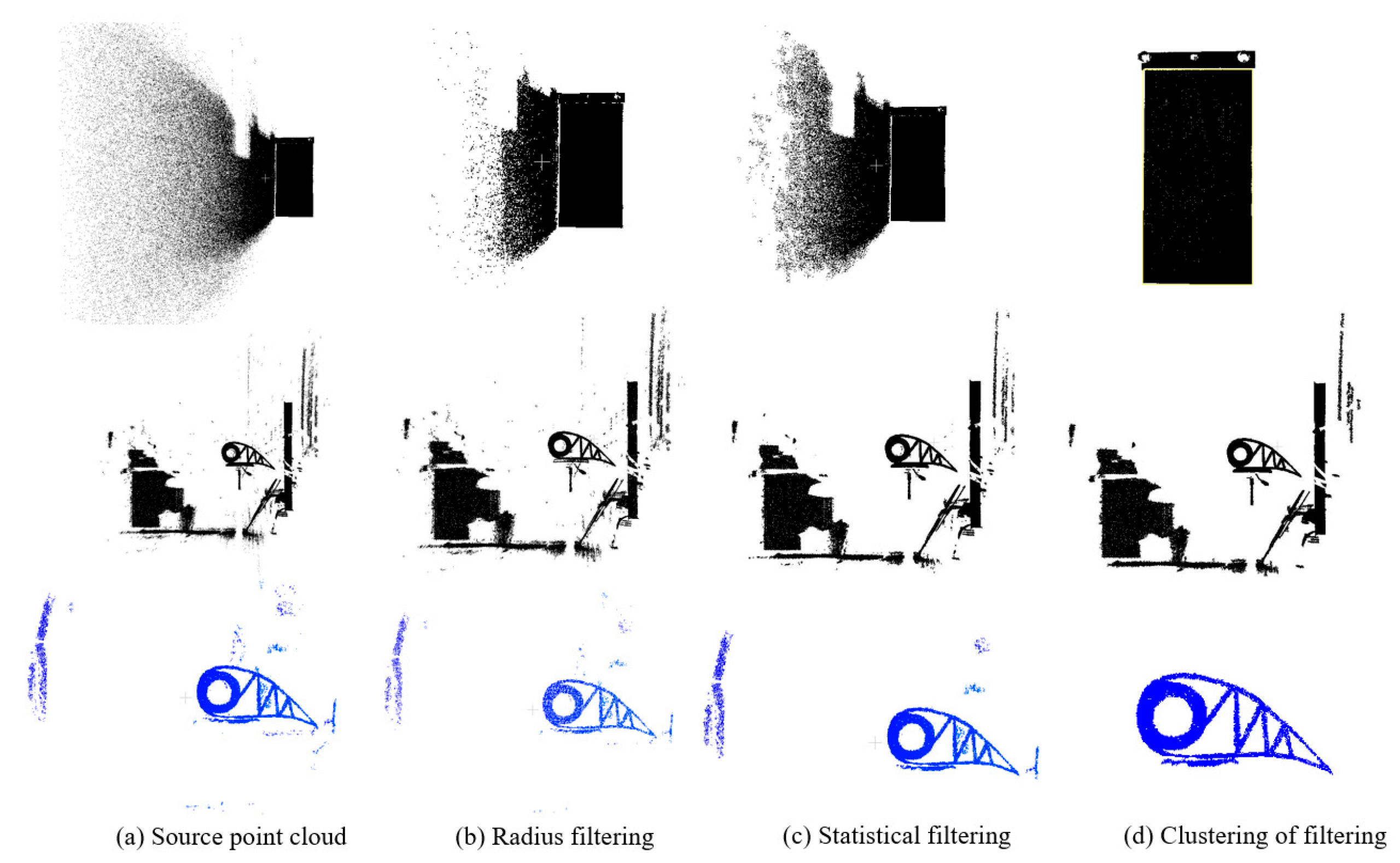
2.1. Point Cloud Preprocessing Part
- (1)
- Firstly, the average distance to the n neighboring points of each point is calculated for point , from which a Gaussian distribution is derived. Next, the mean μ and standard deviation σ of this distribution are determined, the point cloud’s threshold density is set as ρ = n/(μ + σ), and the noise point cloud’s density threshold is established, typically at 18.7% of the point cloud’s density threshold ρ.
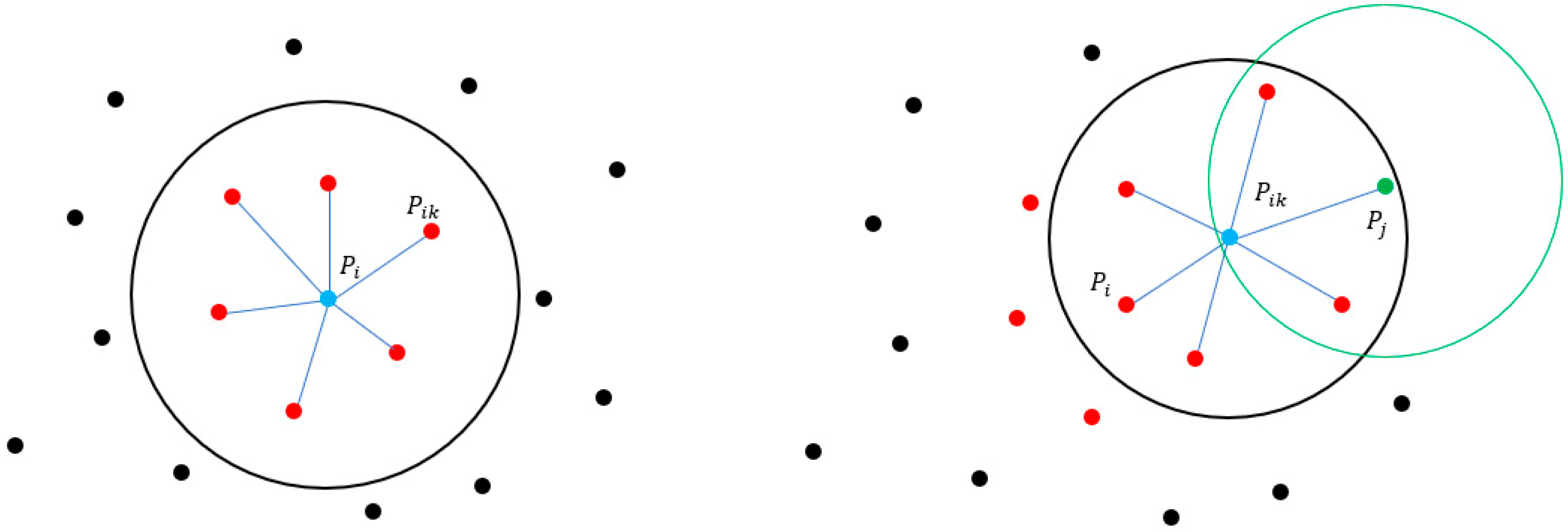
- (2)
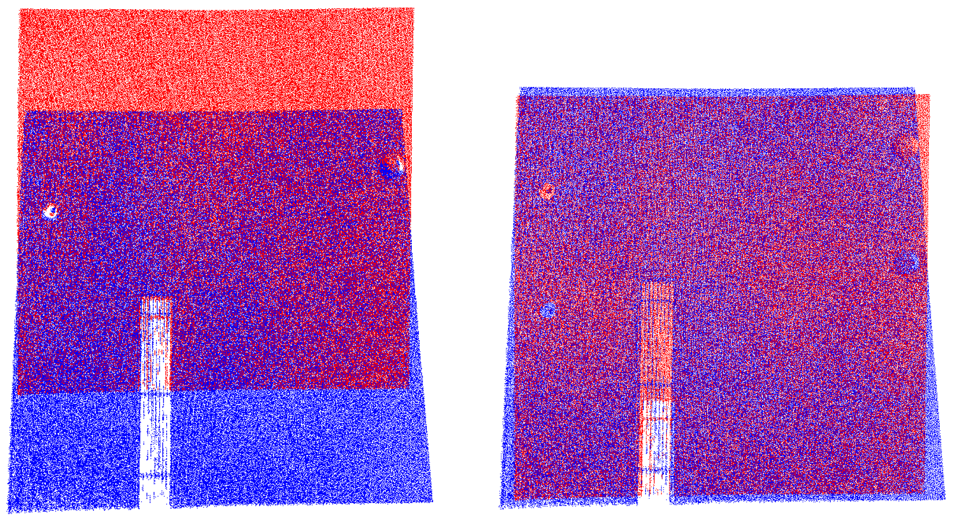
- From the point cloud dataset , select any point and identify the number k (related to the point cloud’s resolution) of points within the search radius around . Calculate the point cloud density ρ = k/R, if ρ exceeds the set threshold for point cloud density, classify as a key point and establish a direct density relationship with associated with . If ρ is below the threshold for point cloud density but above the threshold for noise point density, classify as an edge point. If ρ falls below the noise point density threshold, classify as a noise point. Continue this classification process until all points in the point cloud have been categorized, such as Figure 3 and Figure 4.
- (3)
- Next, select any point from the point cloud, excluding the point already chosen in Step (1), and repeat the process of Step (1). A point , that lies within the neighborhood of but not within the neighborhood of is considered to have a density reachability relationship with . Continue this process as described in Step (3) until the relationships for all neighborhood points of identified in Step (1) are established.
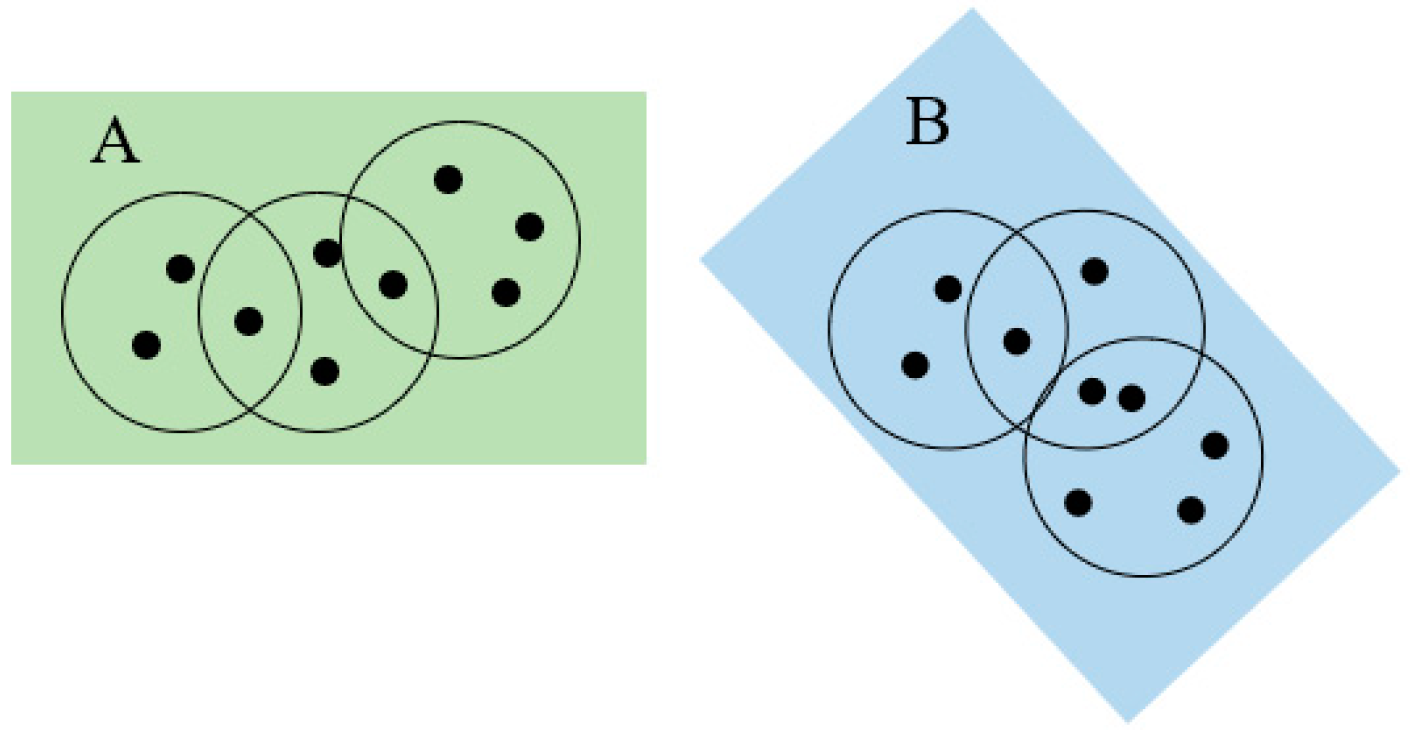
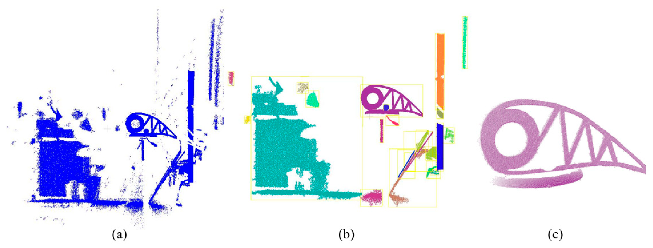
- (4)
- Traverse the point cloud dataset to cluster each point, and group all points that are density-connected into the same cluster, continuing this process until the entirety of the point cloud data have been searched.
2.2. Rough Point Cloud Registration
2.2.1. Normal Vector Estimation
- (1)
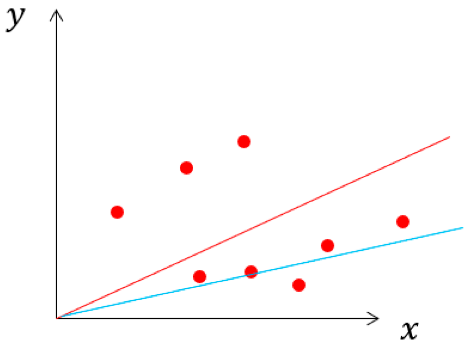
- Calculate the mean value of the point cloud dataset P, where . Given that PCA is highly sensitive to the variance in the initial data variables, de-meaning is essential to prevent distortion of the principal components. Subsequently, project each point onto the plane fitted by least squares, calculate the distance from each point to this plane, and transform the normal vector estimation into the extremum problem as formulated in Equation (6), as Figure 6.where d represents the distance from the centroid point to the best-fit plane.
- (2)
- The covariance matrix M is calculated to represent the correlation between points in a given direction.
- (3)
- The covariance matrix is decomposed into its eigenvalues, which are then ordered from largest to smallest, yielding three distinct eigenvalues , , and . The eigenvector associated with the smallest eigenvalue represents the normal vector to the fitting plane, which is also the normal vector for the point .
- (4)
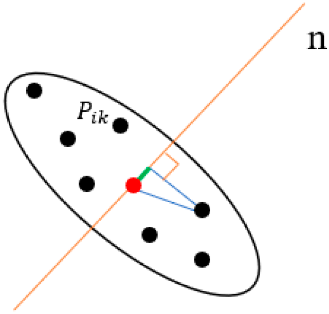
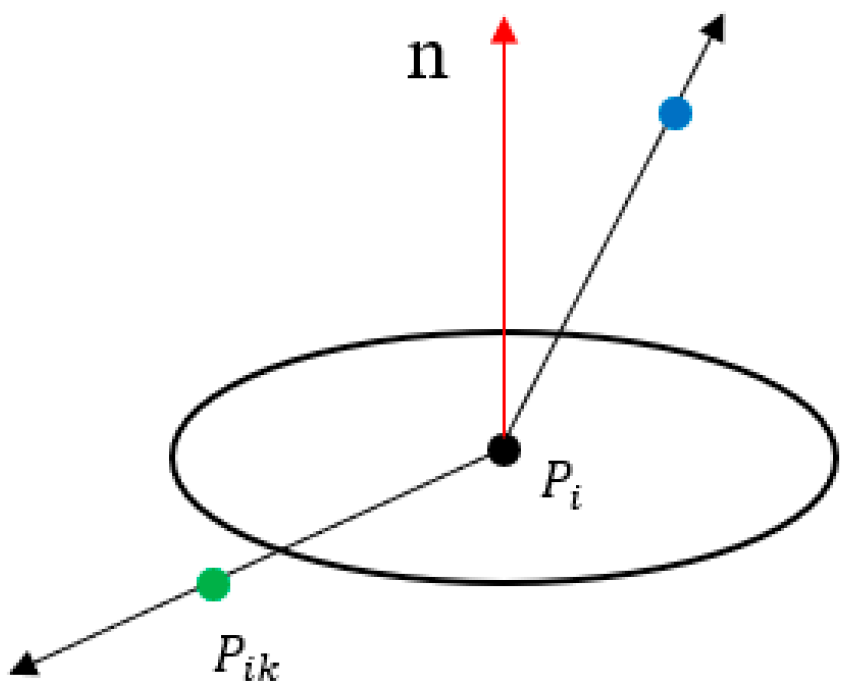
- After the normal vector calculation is completed, its accuracy should be verified by measuring the angle between the estimated normal vector and a reference direction at each point. If this angle significantly deviates from the expected value ideally around 90° then, as depicted in Figure 7, the estimation for that point is deemed inaccurate. In such cases, the outlier point is excluded, and the normal vector is recalculated without its influence.
- (5)
- Given that the normal vector can point in two opposite directions, its orientation must be determined based on the angle it forms with the vector from the centroid to point .The direction of the normal vector is ascertained using this method.
2.2.2. Normal Vector Estimation
- (1)
- Step 1, select n points from the source point cloud dataset . Ensure the distance between each pair of points exceeds a specified threshold to ensure a more uniform sampling that captures a diverse set of features.
- (2)
- Step 2, for each point selected in Step 1, identify a corresponding point in the target point cloud with a similar feature descriptor value, such as a feature histogram eigenvalue.
- (3)
- Calculate the rigid transformation matrix for the corresponding points identified in Step 2. Use the change in the sum of distances between these point pairs after the transformation as a measure of the current transformation’s quality. Continuously refine the matrix, iterating until either the maximum number of iterations is reached or the convergence criteria are satisfied.
2.3. Precise Point Cloud Registration
- (1)
- Firstly, select an arbitrary point from the source point cloud dataset , and calculate the square of the distance to its nearest corresponding point in the target point clouds.
- (2)
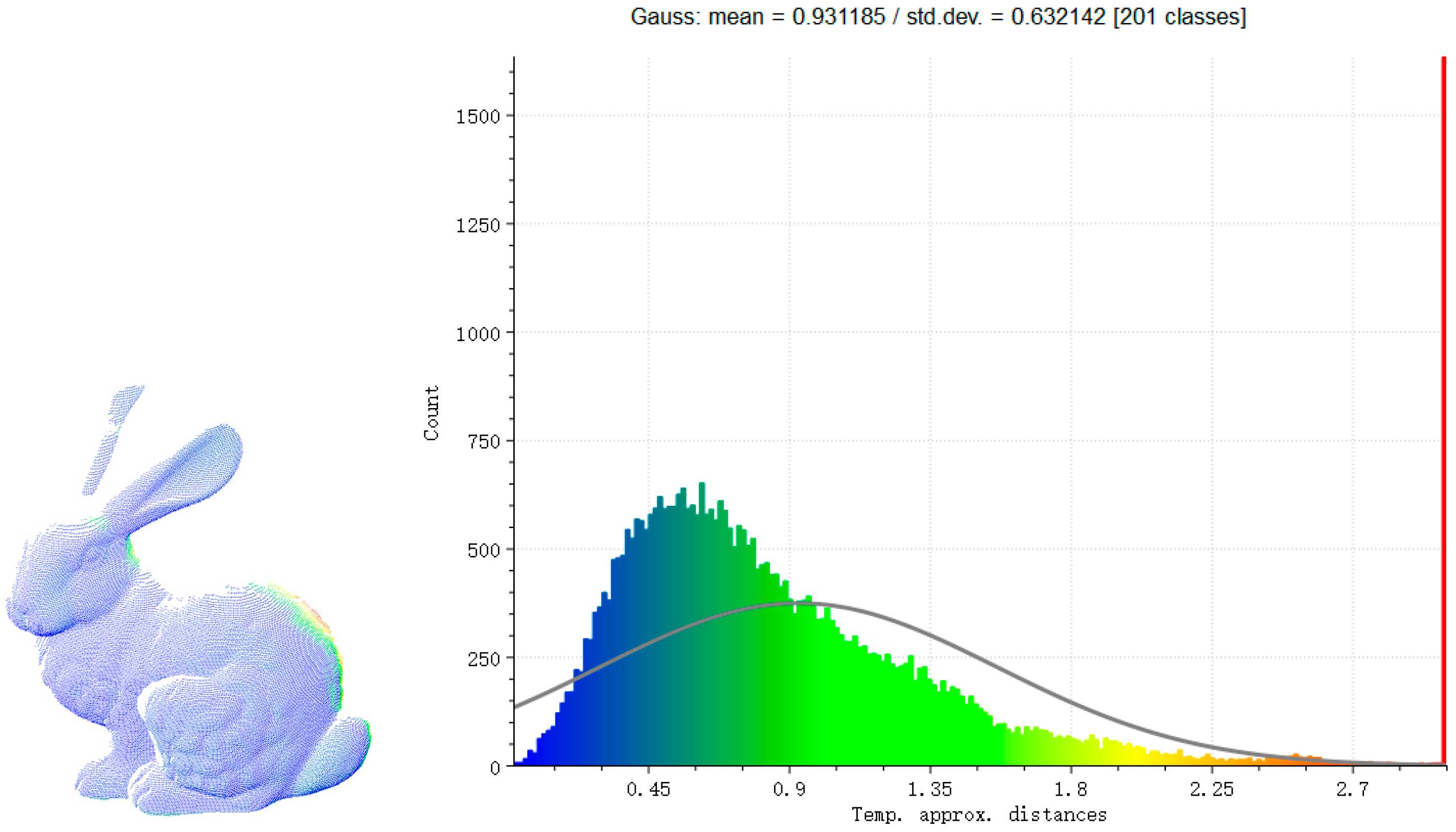
- Calculate the square of the distance between the point and their nearest corresponding points , sort these distances in descending order, and perform a statistical analysis (Figure 10). Establish a threshold at α%, identified from the inflection point relating to the size of the overlap region and the distribution of distances. Select the point pairs that correspond to the first hundredth of α% of the distances, and designate this subset as representing the overlap between the source and target point clouds.
- (3)
- By minimizing the objective function, determine the rotation matrix R and the translation vector t that best align the point clouds.
- (4)
- Apply the 3D transformation matrix to the point . Recalculate the square of the distances between all points in the source point cloud and their nearest points in the target point cloud, sort these distances, and iteratively repeat steps (2), (3), and (4) until the desired accuracy is achieved.
- (1)
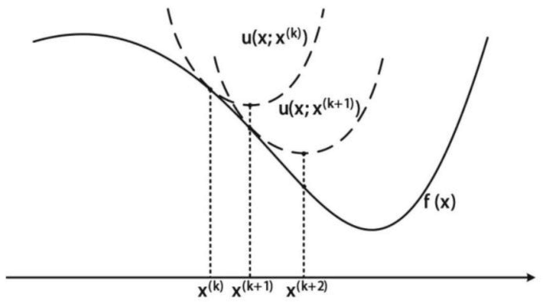
- Identify a surrogate function at the current iteration point that majorizes the original function , ensuring that provides an upper bound for at each point x.
- (2)
- Compute the minimum value of the surrogate function to determine the next iteration point , such that .
- (3)
- Evaluate by substituting into the original function , then proceed with step (1) using the updated surrogate function in place of .
- (4)
- Repeat step (2) to identify the minimum of the surrogate function and continue iterating; this process gradually converges to the minimum of the original function.
3. Results
3.1. Experimental Process
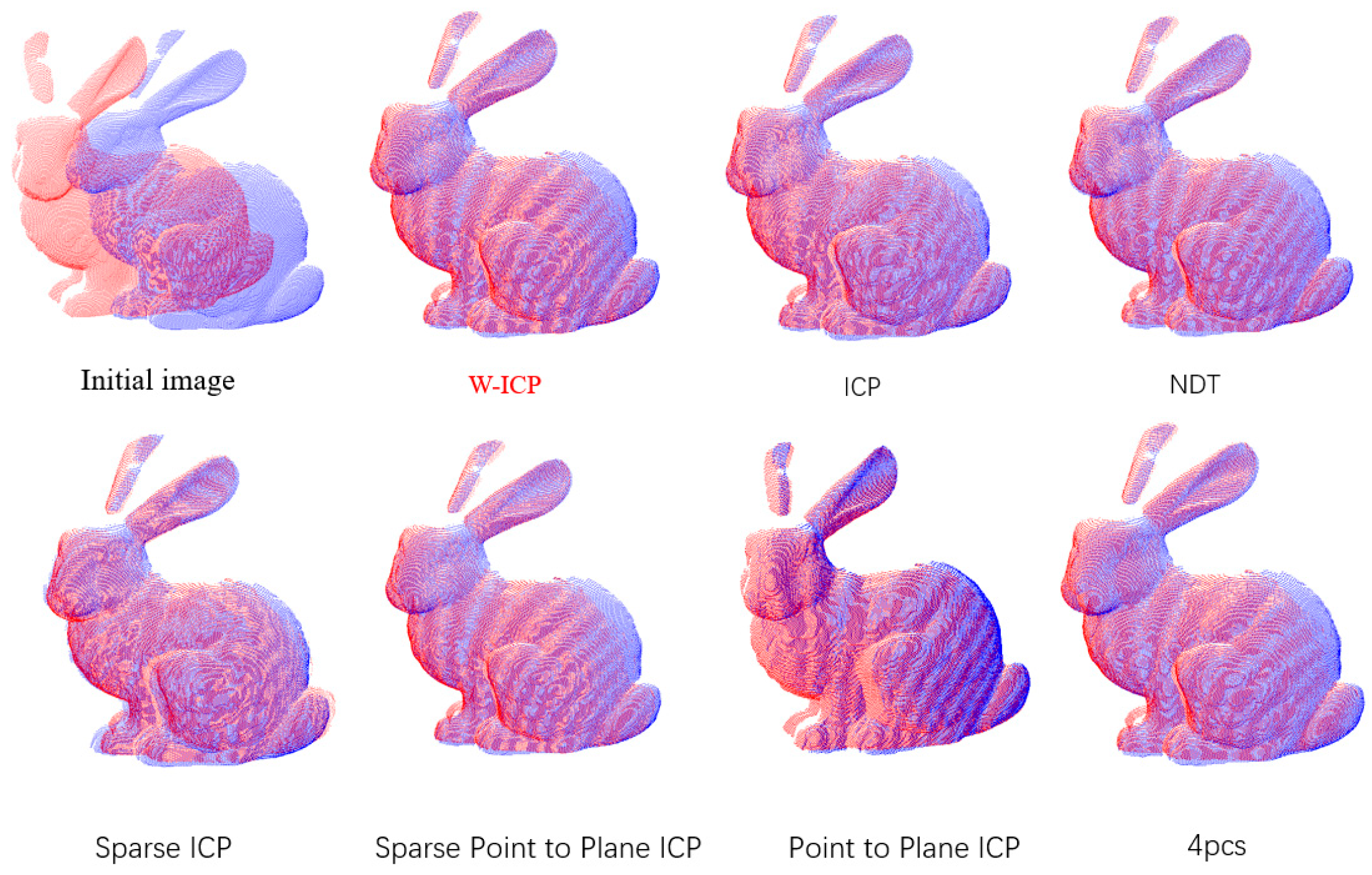
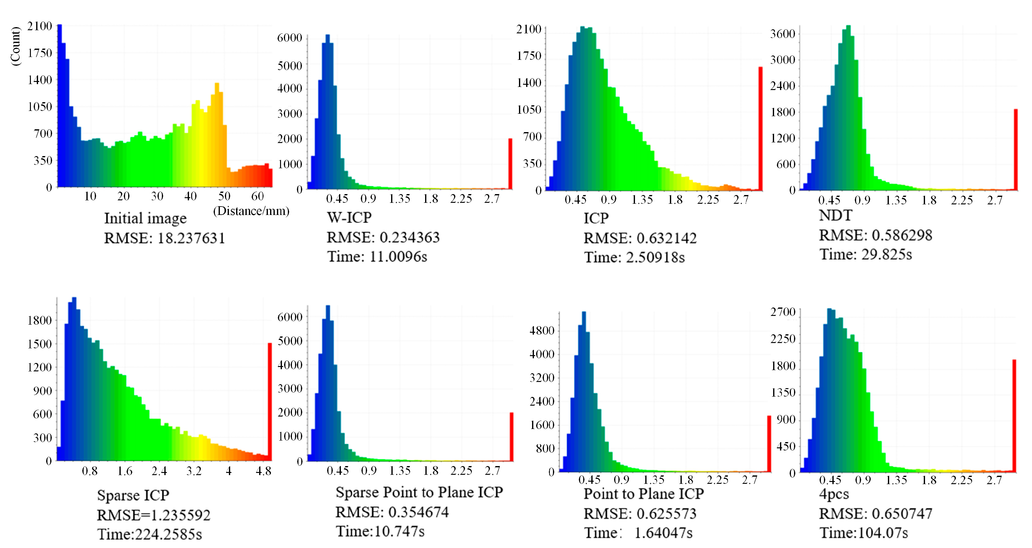
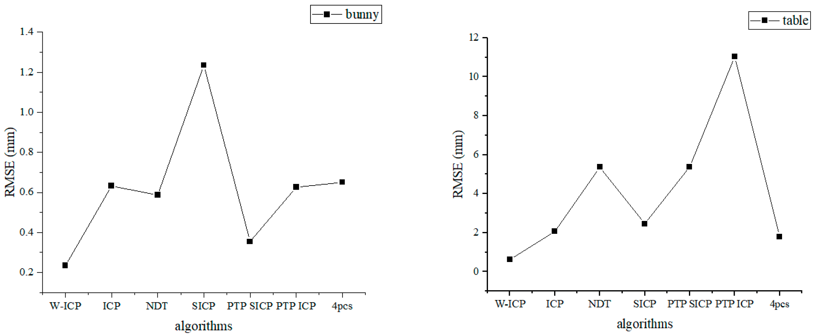
3.2. Dataset Verification
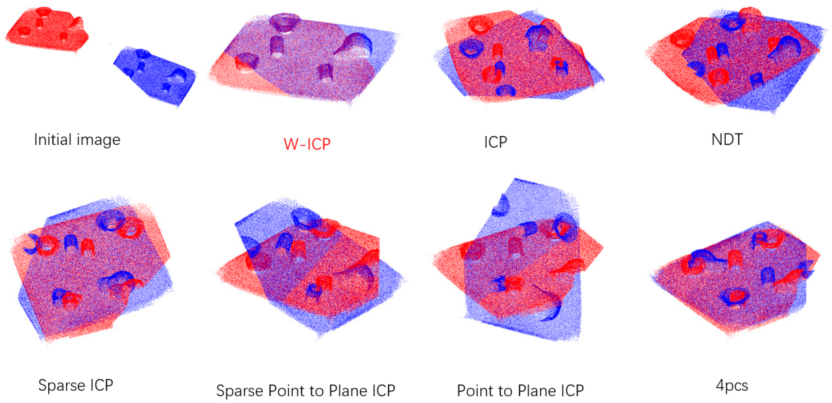
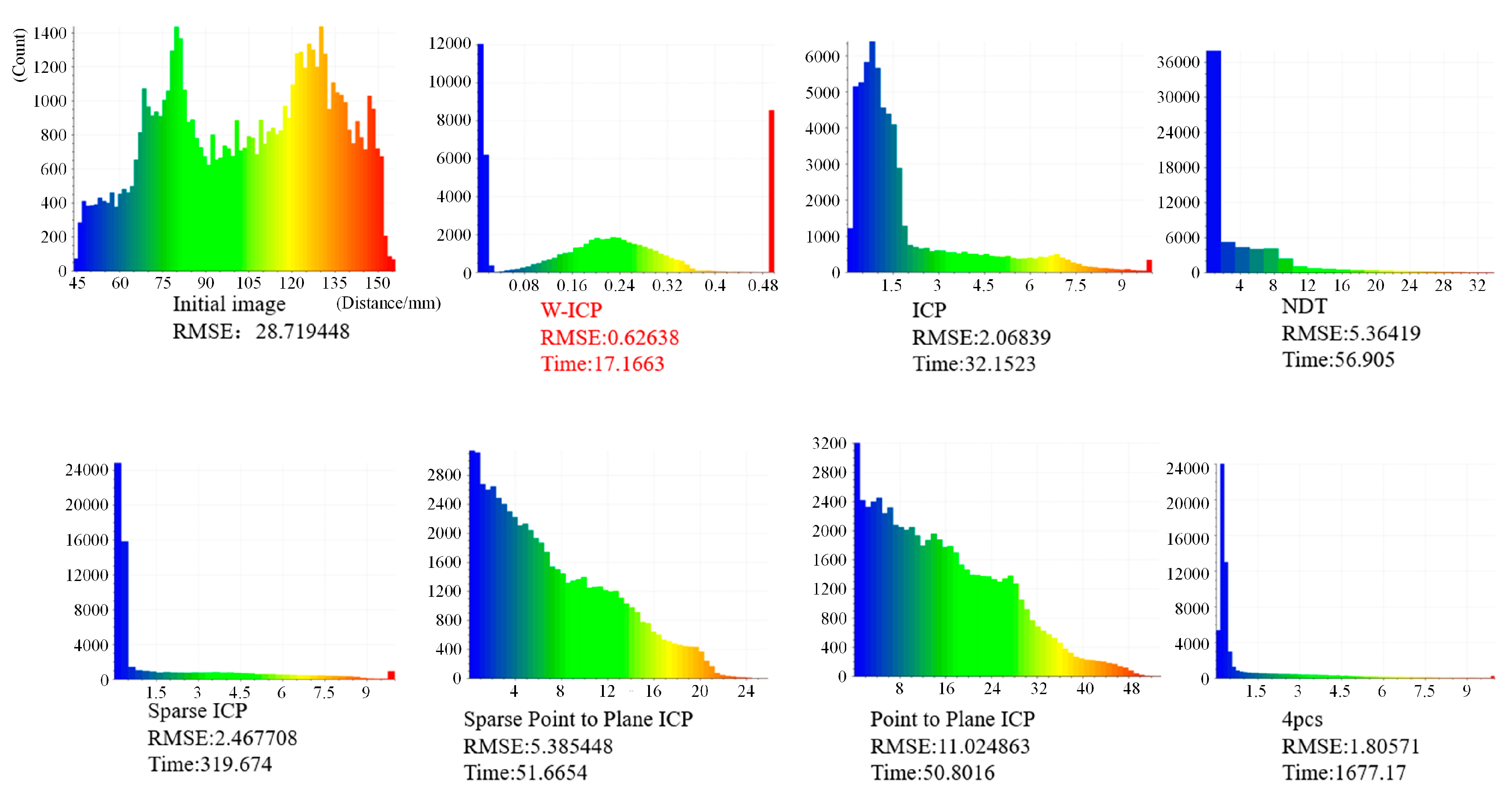
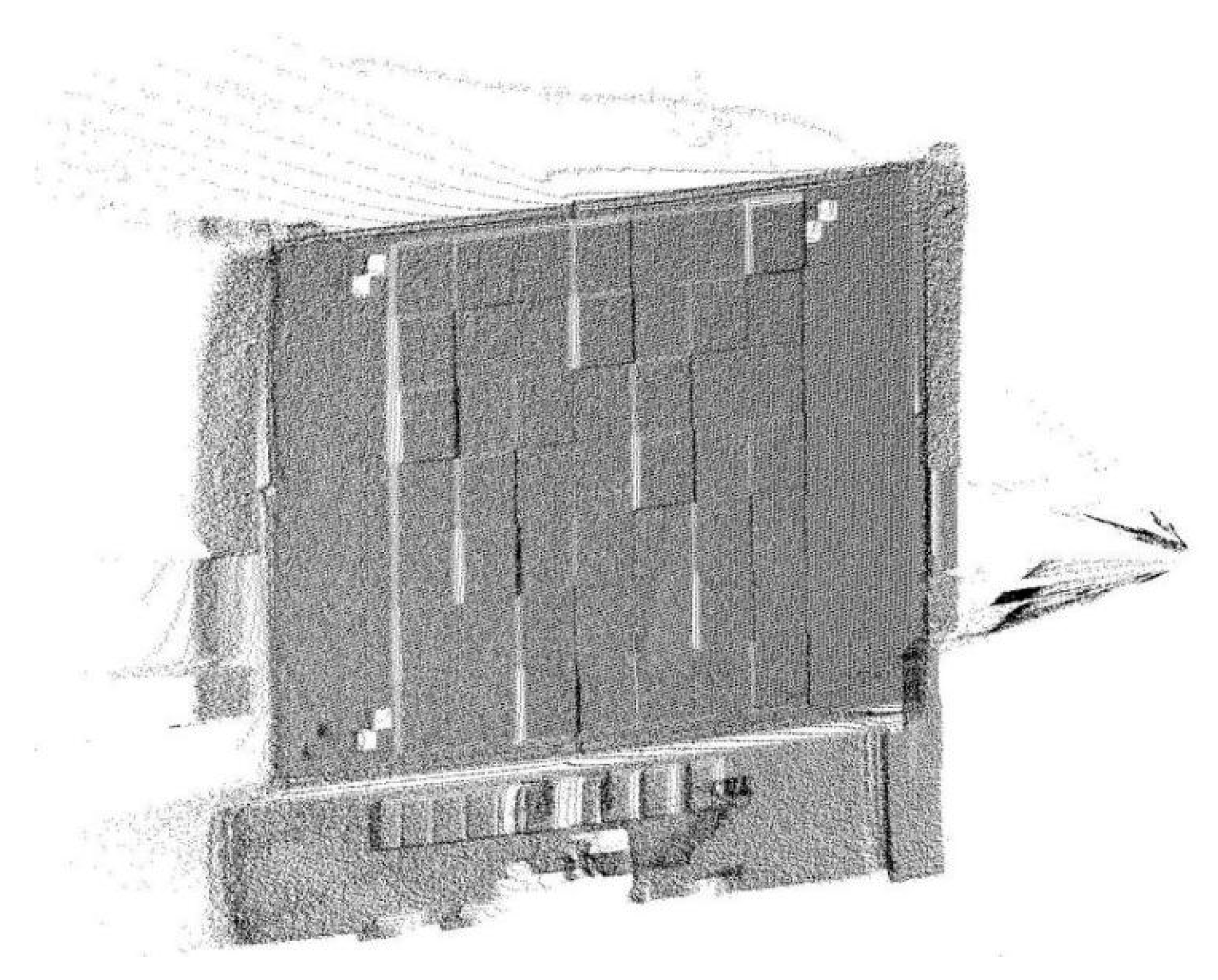
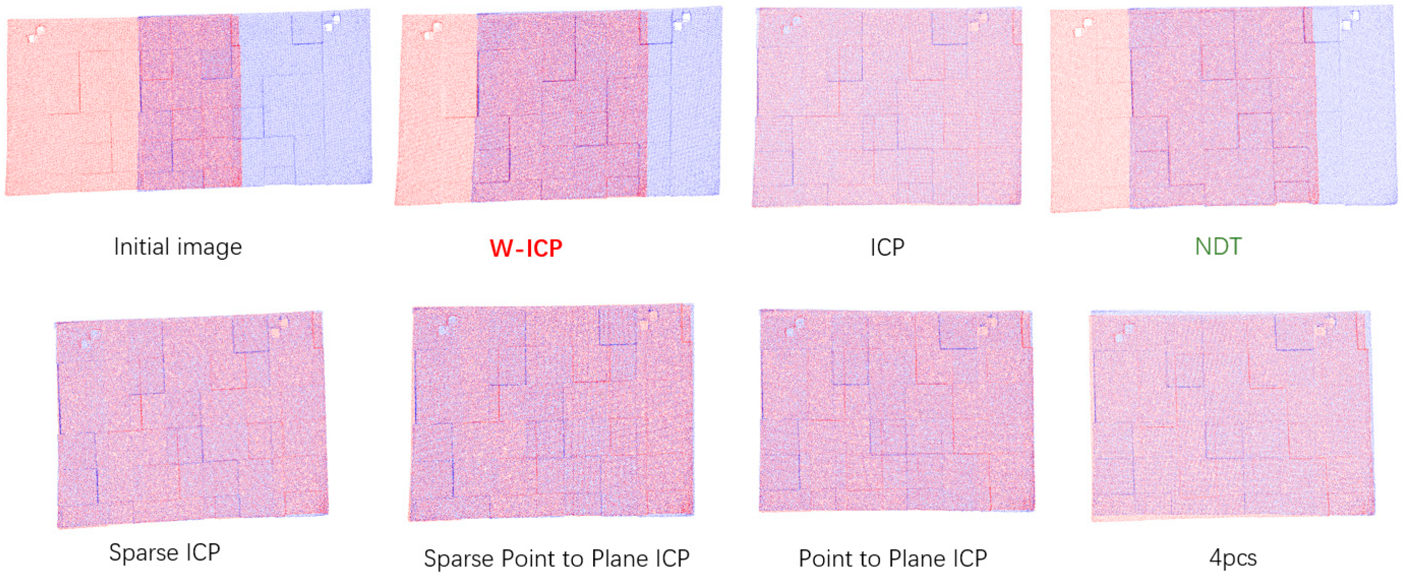
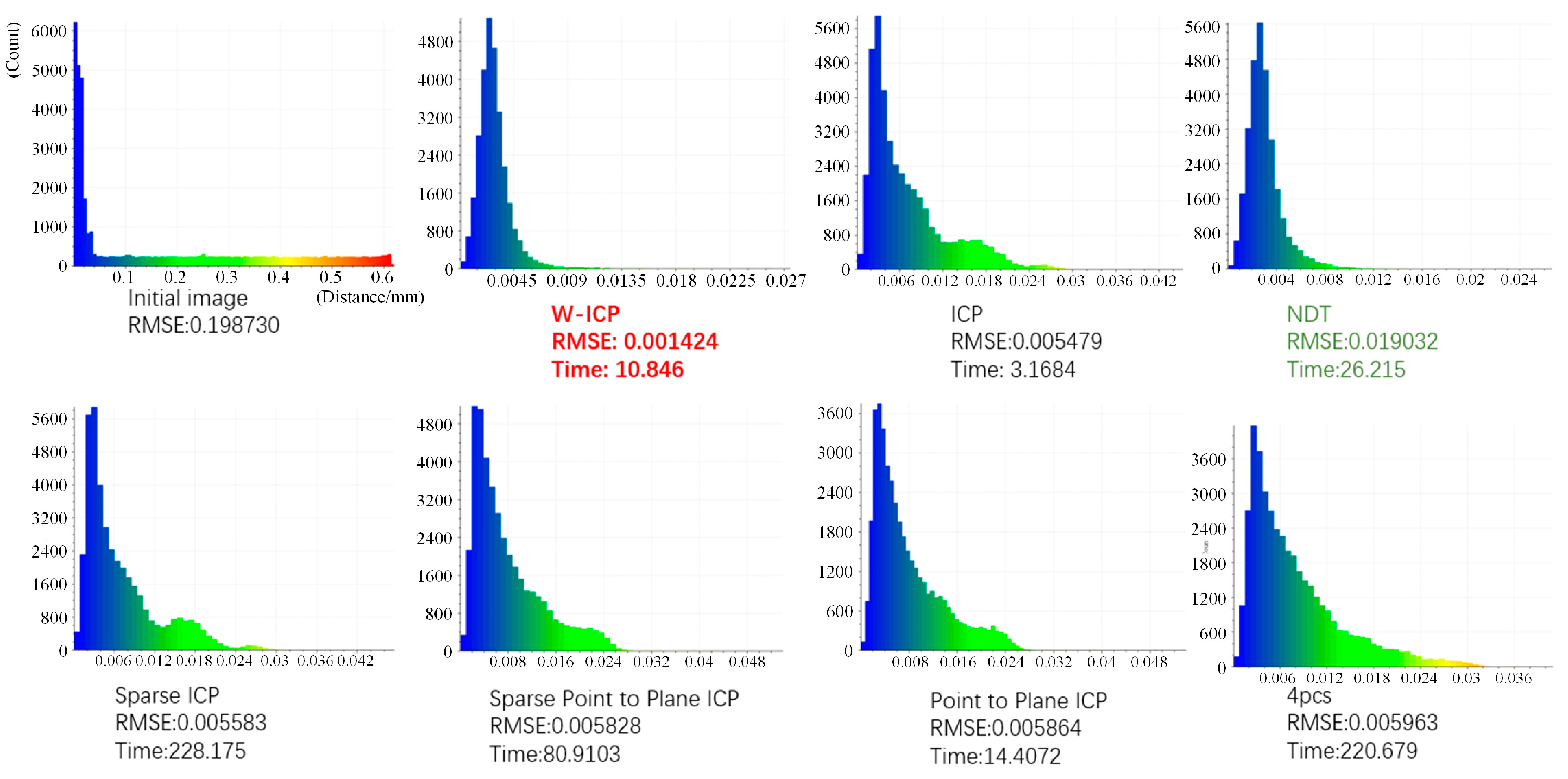
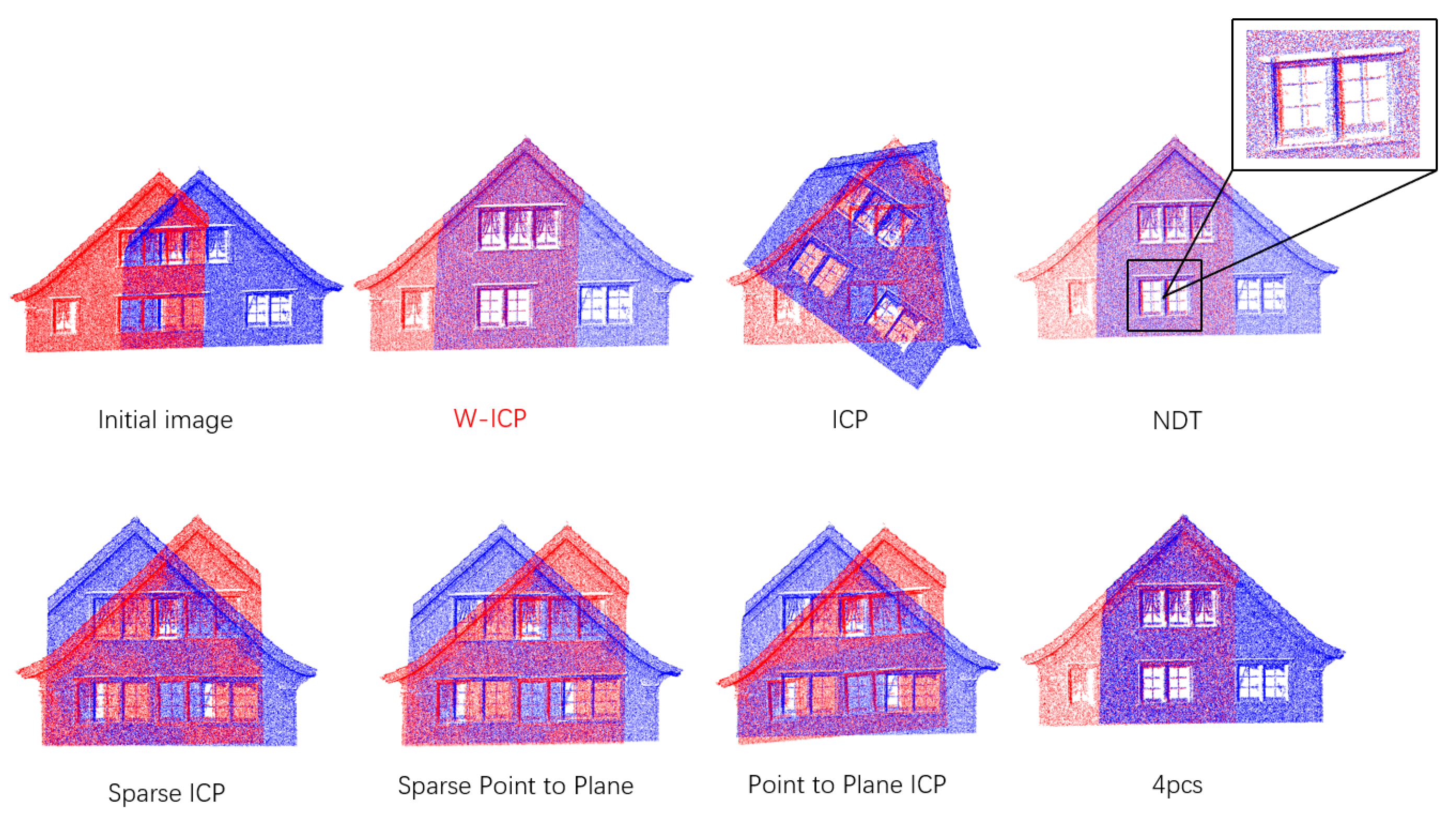
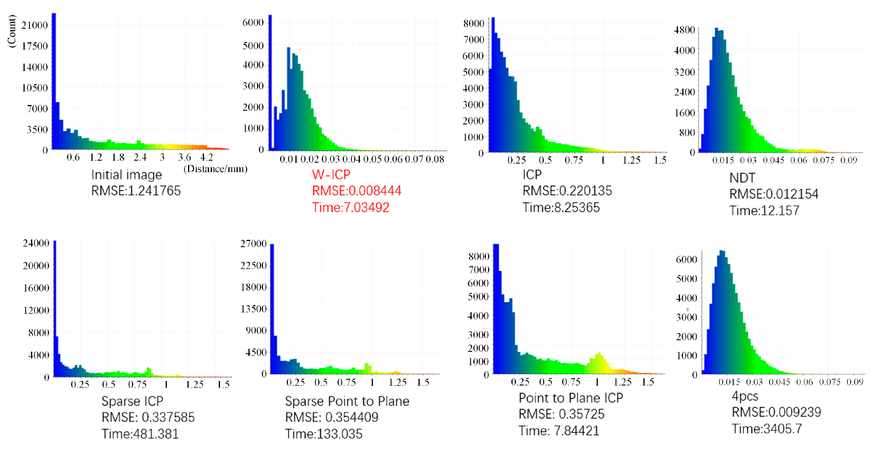
3.3. Verification of Real Shooting Point Cloud Data
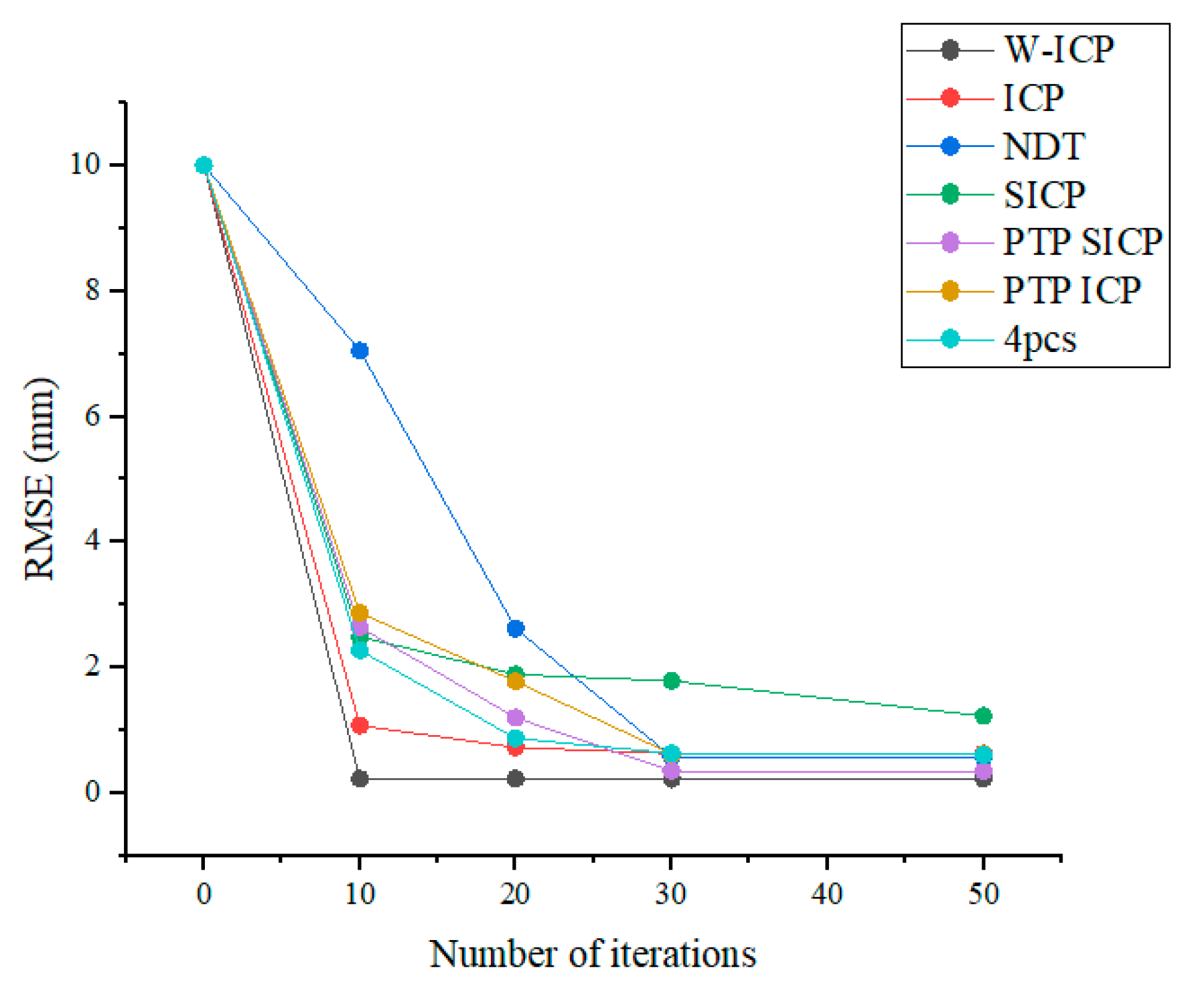
3.4. Comparison of Iterative Convergence Rates
4. Conclusions and Summary
Author Contributions
Funding
Data Availability Statement
Conflicts of Interest
References
- Nurunnabi, A.; Sadahiro, Y.; Laefer, D.F. Robust statistical approaches for circle fitting in laser scanning three-dimensional point cloud data. Pattern Recognit. J. Pattern Recognit. Soc. 2018, 81, 417–431. [Google Scholar] [CrossRef]
- Su, Y.; Hou, M.; Li, S. Three-dimensional point cloud semantic segmentation for cultural heritage: A comprehensive review. Remote Sens. 2023, 15, 548. [Google Scholar] [CrossRef]
- Shen, Y.; Ren, J.; Huang, N.; Zhang, Y.; Zhang, X.; Zhu, L. Surface form inspection with contact coordinate measurement: A review. Int. J. Extrem. Manuf. 2023, 5, 022006. [Google Scholar] [CrossRef]
- Besl, P.J.; Mckay, N.D. A method for registration of 3-D shapes. IEEE Trans. Son Pattern Anal. Mach. Intell. 1992, 14, 239–256. [Google Scholar] [CrossRef]
- Chen, Y.; Medioni, G. Object modeling by registration of multiple range images. In Proceedings of the IEEE International Conference on Robotics and Automation, Sacramento, CA, USA, 9–11 April 1991; pp. 145–155. [Google Scholar]
- Yang, J.; Lih, J. Go-ICP: Solving 3D Registration Efficiently and Globally Optimally. In Proceedings of the 2013 IEEE International Conference on Computer Vision, Sydney, Australia, 1–8 December 2013. [Google Scholar]
- He, Y.; Lee, C.H. An improved ICP registration algorithm by combining PointNet++ and ICP algorithm. In Proceedings of the 6th International Conference on Control, Automation and Robotics (ICCAR), Singapore, 20–23 April 2020; pp. 741–745. [Google Scholar]
- Simon, D.A.; Hebert, M.; Kanade, T. Techniques for Fast and Accurate Intrasurgical Registration. J. Image Guid. Surg. 1995, 1, 17–29. [Google Scholar] [CrossRef]
- Pavlov, A.L.; Ovchinnikov, G.W.; Derbyshev, D.Y.; Tsetserukou, D.; Oseledets, I.V. AA-ICP: Iterative Closest Point with Anderson Acceleration. In Proceedings of the 2018 IEEE International Conference on Robotics and Automation (ICRA), Brisbane, QLD, Australia, 21–25 May 2018; pp. 3407–3412. [Google Scholar]
- Ren, Y.; Zhou, F.C. A 3D point cloud registration algorithm based on feature points. In Proceedings of the 1st International Conference on Information Sciences, Machinery, Materials and Energy, Chongqing, China, 11–13 April 2015; Atlantis Press: Chongqing, China, 2015; pp. 802–806. [Google Scholar]
- Yang, J.; Wang, C.; Luo, W.; Zhang, Y.; Chang, B.; Wu, M. Research on point cloud registering method of tunneling roadway based on 3D NDT-ICP algorithm. Sensors 2021, 21, 4448. [Google Scholar] [CrossRef] [PubMed]
- Zhu, J.; Jin, C.; Jiang, Z.; Xu, S.; Xu, M.; Pang, S. Robust point cloud registration based on both hard and soft assignments. Opt. Laser Technol. 2019, 110, 202–208. [Google Scholar] [CrossRef]
- Zhao, H.; Tang, M.; Ding, H. HoPPF: A novel local surface descriptor for 3D object recognition. Pattern Recognit. 2020, 103, 107272. [Google Scholar] [CrossRef]
- Li, P.; Wang, R.; Wang, Y.; Gao, G. Fast method of registration for 3D RGB point cloud with improved four initial point pairs algorithm. Sensors 2019, 20, 138. [Google Scholar] [CrossRef] [PubMed]
- Yang, J.; Li, H.; Campbell, D.; Jia, Y. Go-ICP: A Globally Optimal Solution to 3D ICP Point-Set Registration. IEEE Trans. Pattern Anal. Mach. Intell. 2016, 38, 2241–2254. [Google Scholar] [CrossRef]
- Wu, Z.; Chen, H.; Du, S.; Fu, M.; Zhou, N.; Zheng, N. Correntropy based scale ICP algorithm for robust point set registration. Pattern Recognit. 2019, 93, 14–24. [Google Scholar] [CrossRef]
- Wu, P.; Li, W.; Yan, M. 3D scene reconstruction based on improved ICP algorithm. Microprocess. Microsyst. 2020, 75, 103064. [Google Scholar] [CrossRef]
- Marchel, Ł.; Specht, C.; Specht, M. Testing the accuracy of the modified ICP algorithm with multimodal weighting factors. Energies 2020, 13, 5939. [Google Scholar] [CrossRef]
- Salti, S.; Tombari, F.; Stefano, L.D. SHOT: Unique signatures of histograms for surface and texture description. Comput. Vis. Image Underst. 2014, 125, 251–264. [Google Scholar] [CrossRef]
- Justusson, B.I. Median filtering: Statistical properties. In Two-Dimensional Digital Signal Prcessing II: Transforms and Median Filters; Springer: Berlin/Heidelberg, Germany, 2006; pp. 161–196. [Google Scholar]
- Pan, J.-J.; Tang, Y.-Y.; Pan, B.-C. The algorithm of fast mean filtering. In Proceedings of the 2007 International Conference on Wavelet Analysis and Pattern Recognition, Beijing, China, 2–4 November 2007; Volume 1. [Google Scholar]
- Tsirikolias, K. Low level image processing and analysis using radius filters. Digit. Signal Process. 2016, 50, 72–83. [Google Scholar] [CrossRef]
- Han, X.-F.; Jin, J.S.; Wang, M.-J.; Jiang, W.; Gao, L.; Xiao, L. A review of algorithms for filtering the 3D point cloud. Signal Process. Image Commun. 2017, 57, 103–112. [Google Scholar] [CrossRef]
- Hoppe, H.; DeRose, T.; Duchamp, T.; McDonald, J.; Stuetzle, W. Surface reconstruction from unorganized points. ACM SIGGRAPH Comput. Graph. 1992, 26, 71–78. [Google Scholar] [CrossRef]
- Rusu, R.B.; Blodow, N.; Marton, Z.C.; Beetz, M. Aligning point cloud views using persistent feature histograms. In Proceedings of the 2008 IEEE/RSJ International Conference on Intelligent Robots and Systems, Nice, France, 22–26 September 2008; pp. 3384–3391. [Google Scholar]
- Rusu, R.B.; Blodow, N.; Beetz, M. Fast point feature histograms (FPFH) for 3D registration. In Proceedings of the 2009 IEEE International Conference on Robotics and Automation, Kobe, Japan, 12–17 May 2009; pp. 1848–1853. [Google Scholar]
- Sorkine-Hornung, O.; Rabinovich, M. Least-squares rigid motion using svd. Computing 2017, 1, 1–5. [Google Scholar]


| RMSE (mm) | Time (s) | |
|---|---|---|
| W-ICP | 0.23436 | 11.009 |
| ICP | 0.63214 | 2.509 |
| NDT | 0.58630 | 29.825 |
| 4PCS | 0.65075 | 104.070 |
| Sparse ICP | 1.23559 | 224.258 |
| Sparse Point-to-Plane ICP | 0.35467 | 10.747 |
| Point-to-Plane ICP | 0.62557 | 1.640 |
| RMSE (mm) | Time (s) | |
|---|---|---|
| W-ICP | 0.62638 | 12.856 |
| ICP | 2.06839 | 32.152 |
| NDT | 5.36419 | 56.905 |
| 4PCS | 1.80571 | 1677.170 |
| Sparse ICP | 2.46771 | 319.674 |
| Sparse Point-to-Plane ICP | 5.38545 | 51.665 |
| Point-to-Plane ICP | 11.02486 | 50.802 |
| RMSE (m) | Time (s) | |
|---|---|---|
| W-ICP | 0.001424 | 10.846 |
| ICP | 0.005479 | 3.168 |
| NDT | 0.019032 | 26.215 |
| 4PCS | 0.005963 | 220.679 |
| Sparse ICP | 0.005583 | 228.175 |
| Sparse Point-to-Plane ICP | 0.005828 | 80.910 |
| Point-to-Plane ICP | 0.005864 | 14.407 |
| RMSE (m) | Time (s) | |
|---|---|---|
| W-ICP | 0.008444 | 7.035 |
| ICP | 0.220135 | 8.254 |
| NDT | 0.012154 | 12.157 |
| 4PCS | 0.009239 | 3405.7 |
| Sparse ICP | 0.337585 | 481.381 |
| Sparse Point-to-Plane ICP | 0.354409 | 133.035 |
| Point-to-Plane ICP | 0.357250 | 7.844 |
| RMSE (mm)/Time (s) | ||||
|---|---|---|---|---|
| 10 (Number of Iterations) | 20 | 30 | 50 | |
| W-ICP | 0.65544/8.180 | 0.23437/8.339 | 0.23437/9.808 | 0.23437/10.735 |
| ICP | 1.08041/0.618 | 0.73169/1.189 | 0.63644/1.591 | 0.63644/2.377 |
| NDT | 7.04746/2.787 | 2.62302/6.477 | 1.90987/7.277 | 0.58630/8.237 |
| 4PCS | 2.27900/262.872 | 0.87899/535.570 | 0.64038/59.202 | 0.61628/1346.594 |
| Sparse ICP | 4.09899/10.808 | 3.89407/22.064 | 3.79135/35.430 | 3.62544/56.304 |
| Sparse Point-to-Plane ICP | 4.20625/20.419 | 4.31974/42.142 | 4.80921/66.075 | 4.80921/66.075 |
| Point-to-Plane ICP | 2.87403/0.768 | 2.78403/1.467 | 2.78400/1.766 | 2.78400/1.792 |
Disclaimer/Publisher’s Note: The statements, opinions and data contained in all publications are solely those of the individual author(s) and contributor(s) and not of MDPI and/or the editor(s). MDPI and/or the editor(s) disclaim responsibility for any injury to people or property resulting from any ideas, methods, instructions or products referred to in the content. |
© 2024 by the authors. Licensee MDPI, Basel, Switzerland. This article is an open access article distributed under the terms and conditions of the Creative Commons Attribution (CC BY) license (https://creativecommons.org/licenses/by/4.0/).
Share and Cite
Geng, H.; Song, P.; Zhang, W. An Improved Large Planar Point Cloud Registration Algorithm. Electronics 2024, 13, 2696. https://doi.org/10.3390/electronics13142696
Geng H, Song P, Zhang W. An Improved Large Planar Point Cloud Registration Algorithm. Electronics. 2024; 13(14):2696. https://doi.org/10.3390/electronics13142696
Chicago/Turabian StyleGeng, Haocheng, Ping Song, and Wuyang Zhang. 2024. "An Improved Large Planar Point Cloud Registration Algorithm" Electronics 13, no. 14: 2696. https://doi.org/10.3390/electronics13142696
APA StyleGeng, H., Song, P., & Zhang, W. (2024). An Improved Large Planar Point Cloud Registration Algorithm. Electronics, 13(14), 2696. https://doi.org/10.3390/electronics13142696