Abstract
We found that a second-order ideal memristor [whose state is the charge, i.e., in ] degenerates into a negative nonlinear resistor with an internal power source. After extending analytically and geographically the above local activity (experimentally verified by the two active higher-integral-order memristors extracted from the famous Hodgkin–Huxley circuit) to other higher-order circuit elements, we concluded that all higher-order passive memory circuit elements do not exist in nature and that the periodic table of the two-terminal passive ideal circuit elements can be dramatically reduced to a reduced table comprising only six passive elements: a resistor, inductor, capacitor, memristor, mem-inductor, and mem-capacitor. Such a bounded table answered an open question asked by Chua 40 years ago: Are there an infinite number of passive circuit elements in the world?
1. Introduction: Chua’s Periodic Table of Ideal Circuit Elements
In 1971, Chua defined the memristor in his seminal paper [1] as a fourth basic two-terminal circuit element, which is characterized by a φ-q curve and an input–output Lissajous figure . Chua also proved a passivity criterion: A memristor characterized by a differentiable charge-controlled φ-q curve is passive if, and only if, its incremental memristance M(q) is nonnegative, i.e., [1]. This criterion shows that only memristors characterized by a monotonically increasing φ-q curve can exist in a device form without internal power supplies [1].
In 1976, Chua and Kang defined a broad generalization of memristors (memristive systems) [2] by
where v, i, and x denote the voltage, current, and state (incorporating the memory effect), respectively. Chua and Kang also provided a passivity criterion (the input–output Lissajous figure always passes through the origin) if and only in for any admissible input current i(t) [2]. In this study, we will use the same passivity criterion (to simply test whether the input–output Lissajous figure passes through the origin, i.e., if or vice versa) for the ideal memristor [1,2].
In 1982, Chua and Szeto introduced higher-order and mixed-order nonlinear circuit elements in a periodic table of all two-terminal nonlinear circuit elements (α, β), that is, periodic modulo ± 4 [3], as shown in Figure 1. They presented that a two-terminal circuit element characterized by a constitutive relation in the v(α)-versus-i(β) plane is called an (α, β) element, where v(α) and i(β) are complementary variables derived from the voltage v(t) and current i(t), respectively [3]. α and β can be any positive integer (representing αth-order or βth-order integral with respect to time), any negative integer (representing αth-order or βth-order integral with respect to time), or zero [3]. They demonstrated that most of the circuit elements in the table are active and not lossless [3]. They predicted that the only nonlinear candidates for passivity are the elements that lie on the three diagonals (in yellow and red), as shown in Figure 1 [3].
In 1984, Chua and Szeto further demonstrated that any higher nonlinear n-port element with a defined constitutive relation can be realized using a mixture of linear elements, nonlinear elements, and power sources [4].

Figure 1.
Chua’s periodic table of all two-terminal nonlinear ideal circuit elements (α, β), that is, periodic modulo ± 4. This table is unbounded since Chua thought he could use his four-element torus (resistor, inductor, capacitor, and memristor) as a seed to generate all other elements endlessly [5]. Chua and Szeto predicted that most of the higher-order circuit elements are active, and the only passive nonlinear candidates are on the three diagonals (in yellow and red) [3].
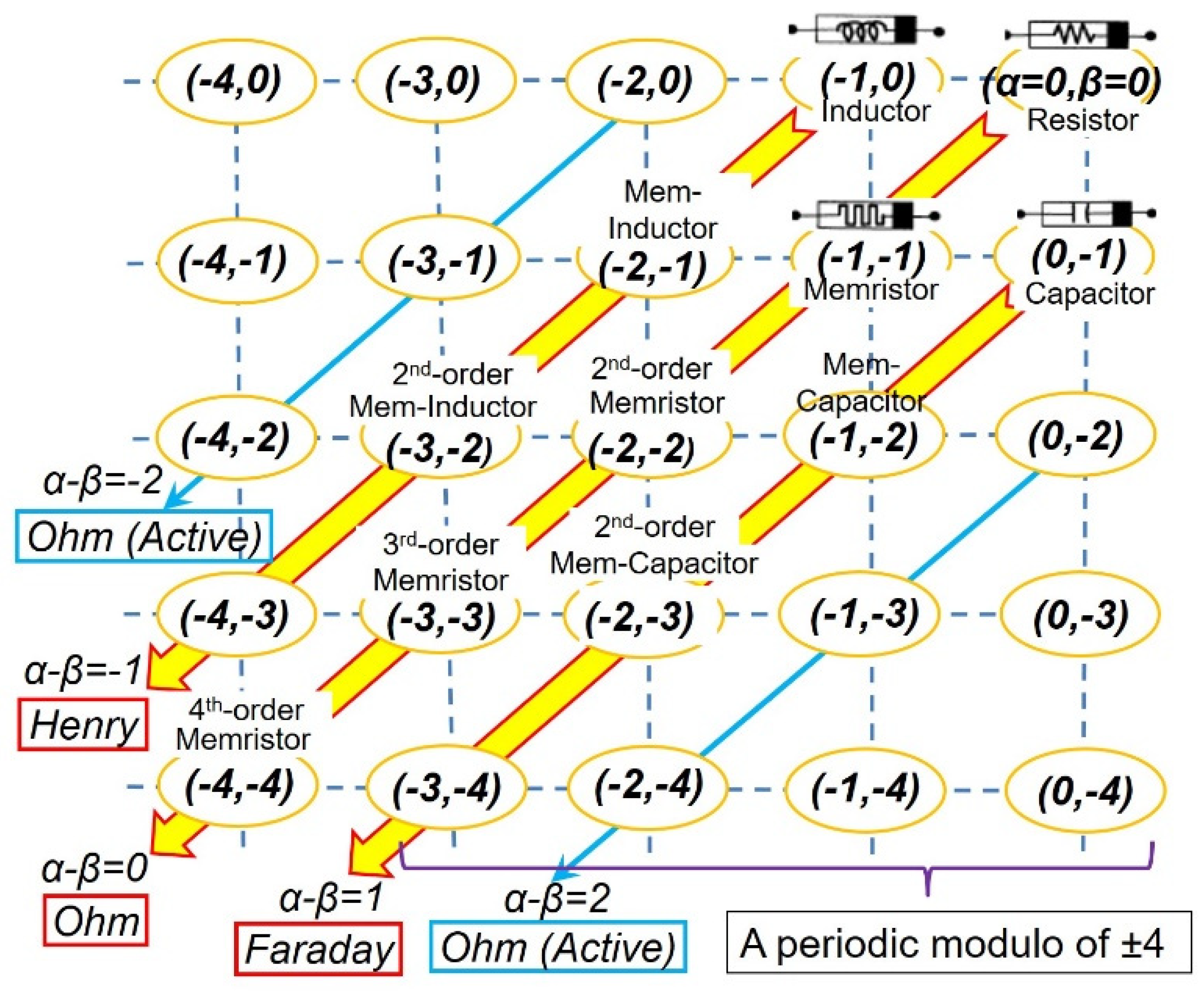
In 2003, Chua defined memristor by the flux as a single-valued function of the charge , namely, [5]. He picked a resistor (α = 0, β = 0), inductor (−1, 0), capacitor (0, −1), and memristor (−1, −1) [1,5] to form a four-element torus and used it as a seed to generate all other (α, β) elements in his periodic table of circuit elements, including higher-order memory circuit elements [memristor (α ≤ −2, β ≤ −2), higher-order inductor (α ≤ −3, β ≤ −2), and higher-order capacitor (α ≤ −2, β ≤ −3)]. Note that this definition associated with his periodic table echoes his original 1971 definition [1] rather than his 1976 definition [2].
In 2009, Biolek, Biolek, and Biolkova defined second-order devices by introducing a pair of new integral variables, namely, and , where φ is the magnetic flux and q is the electric charge [6].
In 2009, Pershin, Ventra, and Chua studied charge-controlled mem-capacitors and flux-controlled meminductors [7]. They defined a general class of u-controlled memory devices by the following relations:
where x denotes a state variable describing the internal state of the system, u(t) and y(t) are any two complementary constitutive variables (i.e., current, charge, voltage, or flux) denoting the input and output of the system, g is a generalized response, and f is a continuous vector function [7].
In 2011, Chua pointed out that the ideal memristor (whose memristance is a function of the charge only) can be expressed by letting “” in state-dependent Ohm’s law [8]. That is, Chua’s ideal memristor in his 1971 definition [1] is a special case of his 1976 generic definition [2]. He also stated that a nonlinear memristor is charge-controlled (or flux-controlled) if its constitutive relation can be expressed by , where is continuous and piecewise-differentiable functions with bounded slopes [8]. Again, Chua presented his periodic table of circuit elements [5] in this paper [8]. Obviously, Chua’s (α, β) elements in his periodic table of circuit elements refer to the ideal ones that can be described by a monotonically increasing, continuous, and piecewise-differentiable constitutive curve with bounded slopes and thereby an input–output Lissajous figure . It is worth mentioning that the three ideality criteria summarized by Georgiou [9] agree with Chua’s statement in this paper [8].
In 2012, Chua, et al. demonstrated that the time-varying sodium conductance in the Hodgkin–Huxley circuit is a second-order active sodium memristor with an internal battery [10,11].
In 2013, Riaza demonstrated that the corresponding second order mem-circuits based on those second-order elements yield rich dynamic behavior (e.g., bifurcation phenomena) [12].
In 2013, Mainzer and Chua characterized local activity/local passivity in their book “Local Activity Principle: The Cause of Complexity and Symmetry Breaking” [13]. Actually, this “local passivity” definition is equivalent to the origin-crossing signature used by Chua in 1976 [2] for an ideal memristor. In principle, local activity can be used in a mathematically rigorous way to explain the emergence of complex patterns in a homogeneous medium, such as nonlinear electronic circuits.
In 2014, Georgiou et al. used a non-ideal model to extend Chua’s set of ideality criteria (nonlinear, continuously differentiable, and monotonically increasing) [1] to a new set (nonlinear, continuously differentiable, and strictly monotonically increasing) [9] for the ideal memristor characterized with a φ-q curve [1].
In 2019, Biolek, Biolek, and Biolkova proved that Hamilton’s variational principle still holds true for circuits consisting of (α, β) elements from Chua’s periodical table [14].
In 2019, Chua classified all memristors into three classes called Ideal, Generic, or Extended memristors [15].
In 2021, Corinto, Forti, and Chua further characterized passivity (for any shape of the signal) in their book “Nonlinear Circuits and Systems with Memristors” [16].
The paper is structured as follows. In Section 1, we have chronically reviewed the two definitions of the memristor (the ideal memristor and the memristive systems as a broad class) and highlighted the fact that Chua’s periodic table comprises only the ideal circuit elements ( or for the ideal memristor) [15,17]. In Section 2, we will use a first-order ideal memristor as an example to demonstrate the local passivity concept. In Section 3, we will use a generic analytical proof with any possible signals and general constitutive variables (x, y) to investigate whether a second-order memristor (α = −2, β = −2) is locally active. In Section 4, we will use a graphic method to verify the analytically verified local activity of a higher-order memristor in the preceding section. In Section 5, we will demonstrate that a higher-order ideal inductor is locally active. In Section 6, we will demonstrate that a higher-order ideal capacitor is locally active. In Section 7, we will provide an experimental verification based on the famous Hodgkin–Huxley circuit to support our new theory. In Section 8, we will answer an open question in circuit theory: Is a single-valued, nonlinear, continuously differentiable, and monotonically increasing constitutive curve locally active?
2. A First-Order Ideal Memristor Is Locally Passive
Notwithstanding the common knowledge that a first-order ideal memristor is locally passive [1], this section is intended to list all the relevant facts for information integrity and prepare some necessary prerequisites for the following sections.
First-order circuit elements are those defined by their constitutive attributes φ and q [1,2,3,4,5,8]. The memristor, with memristance M, provides a constitutive relation between the charge q and the flux φ as given under dφ/dq = M(q, t) memristance. The conformal differential transformation [5] from the original φ-q plane to the v-i plane is shown in Figure 2.
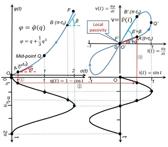
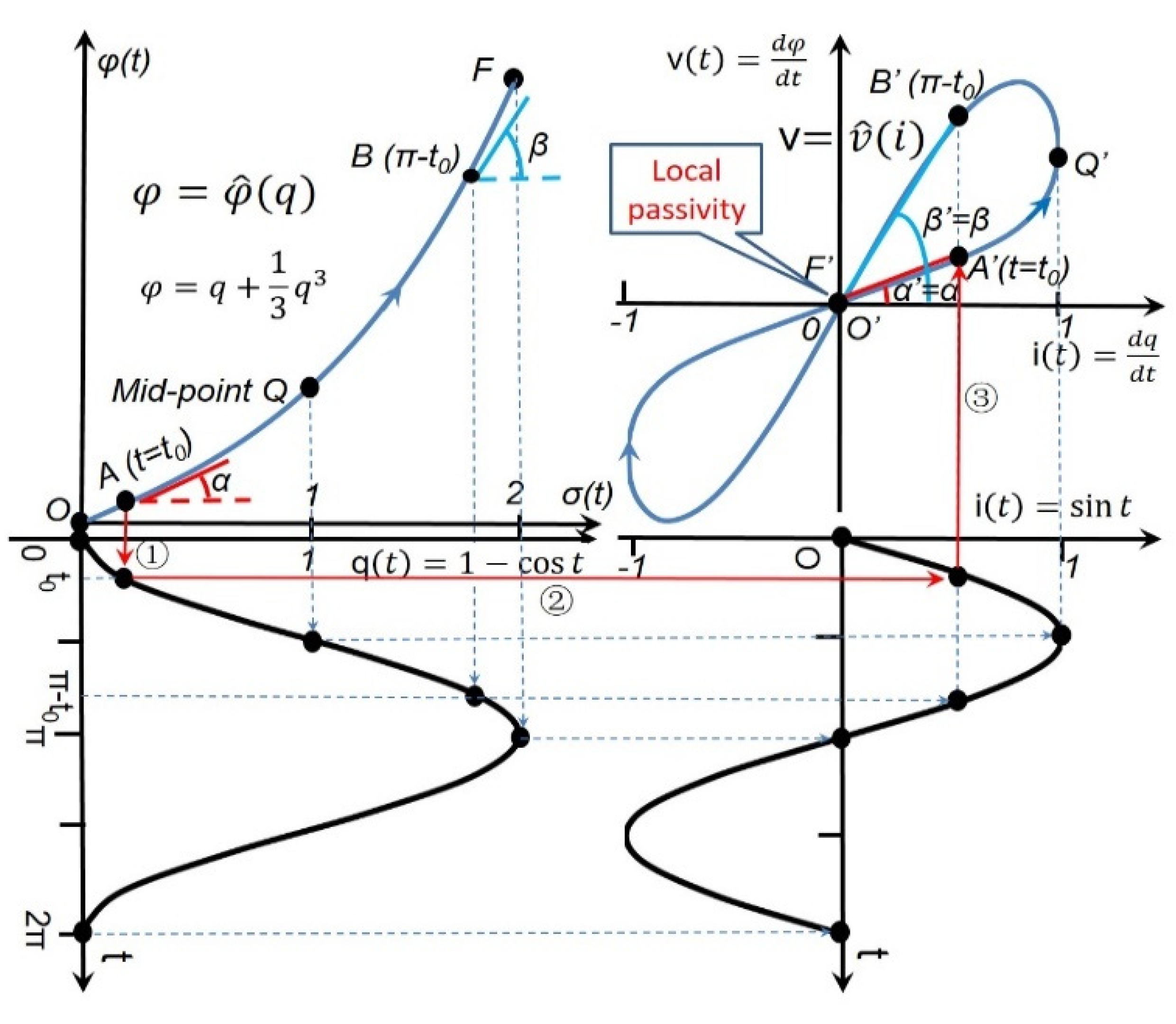
Figure 2.
First-order ideal memristor with a single-valued, differentiable, monotonically increasing curve and an odd-symmetric pinched v-i hysteresis loop against the origin. Based on a “conformal differential transformation” that preserves angles between and , projection lines 1, 2, and 3 denote a simple graphic method to project a given curve in the φ–q plane onto the v-i plane. A′ denotes A’s projected point after one transformation, and so on. A small region (e.g., the short arc above Q′) with a negative slope does not imply that there is an internal power source inside this first-order memristor [8]. Rigorously speaking, this graphic approach is vivid but inadequate since the passivity of a circuit element refers to any possible shape of the excitation. A strict, generic analytical proof for any possible shape of the excitation can be found in Section 3.
As shown in Figure 2, an arbitrary curve in the φ-q plane represents an ideal memristor. This curve goes through the origin as . Note that the memristor shown in Figure 2 is charge-controlled, but the principles found here should be applicable to another type of flux-controlled memristor. In Figure 2, and are continuous and piecewise-differentiable functions with bounded slopes [8]. Note that the voltage v is a function not only of i but also of q; therefore, should be a double-valued function of the current i because every pair of points A(t0) and B(π-t0) on the curve (that are subject to the same amplitude of an excitation current) are separated vertically by following their own chord slopes in the v-i plane (to be detailed later).
A cosine charge function is used to cover the full operating range {0, 2}, as used by Chua [8]. Note that only full-range scanning can expose a distinctive “fingerprint”; otherwise, the obtained fingerprint is incomplete. This function is defined by
where the initial charge q(0) = 0.
The corresponding current, i(t), as a testing signal across the memristor, is as follows:
The coordinates of the v-i plane are the differential (with respect to time) of the coordinates of the φ-q plane [5]; hence, we have the following:
That is, the slope (α) of the line tangent to the curve at an operating point A(t = t0) in the φ-q plane equals the slope (α′) of a straight line connecting the projected point A′(t = t0) to the origin in the plane (on the same scale as the φ-q plane) [8].
This conformal differential transformation can be deduced as follows. Linearizing at A(φ0, q0) at t0 (Figure 2) via series expansion, we obtain for the tangent at A(φ0, q0). Differentiating the above equation with respect to time, we obtain that describes the line joining the origin to A′ at t0 in the v-i plane. So, the slopes match.
In Figure 2, we use a graphic method to draw the voltage-current loci corresponding to . (1) We obtain α at an operating point A(t = t0) in , and then draw a straight line through the origin in the v-i plane, whose slope is α′ = α. (2) We project point A(t = t0) from the φ-q plane onto the v-i plane by following Projection Lines ①, ②, and ③, and end up with the same time point A′(t = t0) in the v-i plane by meeting Projection Line ③ with the drawn line in the first step.
As shown in Figure 2, from an arbitrary curve, we obtain an ideal memristor meeting the distinctive fingerprint/signature [8]. 1. Zero-crossing or pinched ( whenever i = 0). 2. Double-valued Lissajous figure.
If the curve is split into two branches (the outgoing path does not overlap the returning path), the pinched figure becomes asymmetric with respect to the origin, as shown in Figure 3. This represents a wide range of real-world non-ideal memristors with an asymmetric bipolar or unipolar pinched Lissajous figure [9].
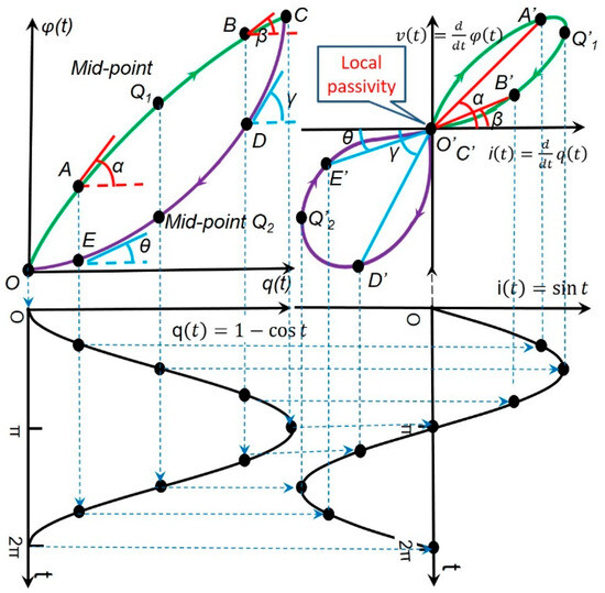
Figure 3.
Georgiou et al. used a real-world memristor with two φ-q characteristic branches (in different colors) and an asymmetric pinched v-i hysteresis loop as a non-ideal example to highlight their set of requirements (nonlinear, continuously differentiable, and strictly monotonically increasing) for the ideal memristor [9]. Note that each branch of the φ-q curve generates only one loop of the Lissajous figure (i). Local passivity [13,15,16] is validated by the origin-crossing fingerprint/signature of the v-i loci. This simple passivity criterion (to simply test whether the input–output Lissajous figure passes through the origin, i.e., if or vice versa) was originally proposed by Chua and Kang in 1976 [2].
A first-order ideal memristor is characterized by a time-invariant φ-q curve complying with the following four criteria:
- Single-valued*;
- Nonlinear;
- Continuously differentiable;
- Strictly monotonically increasing.
Criteria 2–4 for the ideality were extracted from references [1,9]. The only exception is that we added the “single-valued” criterion. *Strictly speaking, if a curve is strictly monotonically increasing, it is single-valued. Listing the “single-valued” criterion separately is performed to clearly exclude the special case (Figure 3), in which a non-ideal memristor has a double-valued, strictly monotonically increasing φ-q curve. In addition, zero initial states [] are assumed as Chua did [1,2,5,8].
The following passivity theorem for a first-order ideal memristor is, therefore, reasoned:
Theorem 1. (Local Passivity Theorem).
A first-order ideal memristor is locally passive.
Proof.
Criteria 4 (strictly monotonically increasing) means that if A < B and f(A) < f(B) by monotonicity, the slope of is nonnegative; hence, this ideal memristor is locally passive at each point on the φ-q curve. This theorem is generic for any possible shape of the excitation. □
This theorem is important for small-signal circuit analysis since a locally active memristor may give rise to oscillations, and even chaos [8]. On the other hand, such passivity leads to energy efficiency in green computing because one does not have to keep supplying power to make a passive circuit element function (in contrast, an active-transistor-based memory cell will lose its stored information after the power supply is switched off).
The coincident zero-crossing signature [15,18,19] is well used for identifying passive devices and it is equivalent to Chua’s local passivity [13] for an ideal circuit element.
Such local passivity should be applicable to both first-order inductors and capacitors. The proof is omitted here due to similarity and simplicity. The reader should perform a deduction similar to that described in Figure 2.
3. A Higher-Order Ideal Memristor Should Be Locally Active: An Analytical Proof with Any Possible Shape of the Excitation
In this section, we will use a second-order memristor (α = −2, β = −2) as an example to study whether it has to be locally active. Rigorously, the passivity of a circuit element refers to any possible shape of the excitation, as originally defined by Chua [13,15,16]. A generic analytical proof with the two general constitutive variables (x, y) for any possible signals will be provided. We will first present the reader with a generic proof (for any form of excitation) and then exemplify it with a sinusoidal signal in the next section.
A cell is said to be locally passive at a cell equilibrium point if, and only if, it is not locally active at that point [13]. Here, a proof is provided as below: a cell is said to be locally active at a cell equilibrium point if, and only if, there exists a continuous input time function , such that at some finite time , and there is net energy flowing out of the cell at , assuming the cell has zero energy at t = 0. Namely, the energy transmitted by the external power supply to the cell is defined as , which means that there is a net energy flowing out of the cell. For all continuous input time functions and for all , is a solution of the linearized cell state equation about with zero initial state and [13]. If or vice versa, there should be an intersectional point crossing either the axis or the axis, which implies that the v-i curve must inevitably enter either the second or the fourth quadrant of the v-i plane. Therefore, a cell with or vice versa must be locally active: .
In order to deal with any possible signals that can be applied, we will use general constitutive variables (x, y). An analytical proof begins with a basic axiom or definition (in this case, it is the definition of the ideal memristor) and reaches its conclusion through a sequence of deductions and mathematical reasoning. As can be seen later, the so-called analytical method will provide a mathematically different and independent proof from a graphical method to be conducted in Section 4.
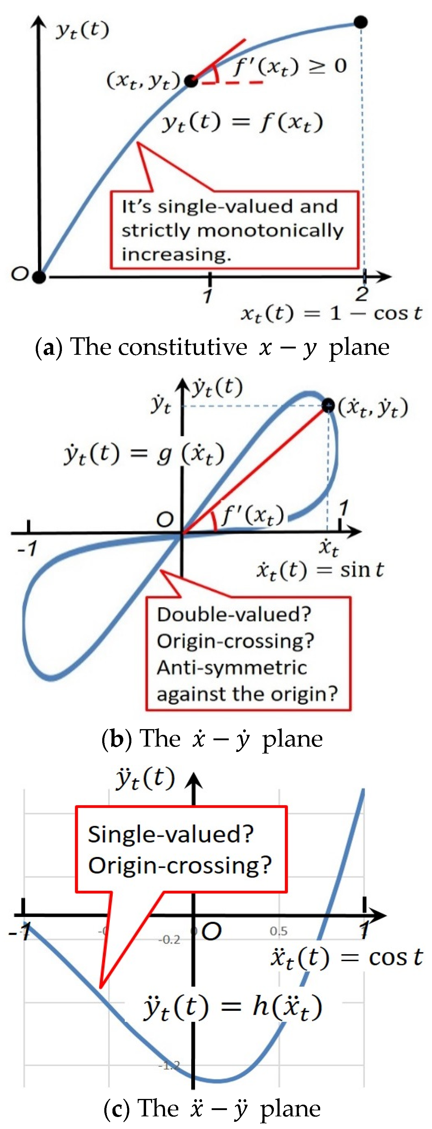
As shown in the constitutive plane in Figure 4a, a second-order ideal memristor is characterized by a time-invariant constitutive curve that is single-valued, nonlinear, continuously differentiable, and strictly monotonically increasing [8,9].
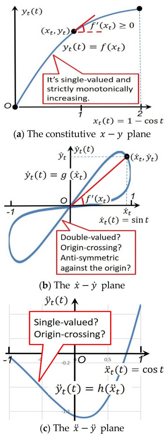
Figure 4.
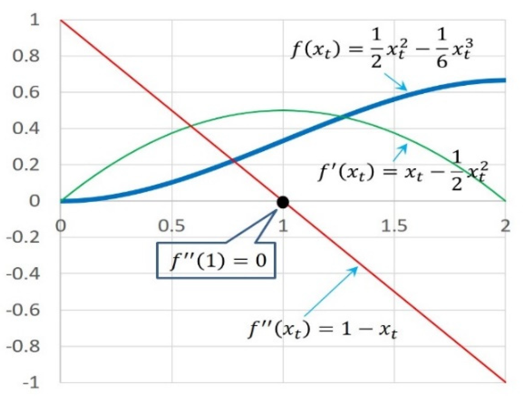
An analytical method is used to verify the local activity of a second-order ideal memristor with general constitutive variables (x, y). The use of a subscript t means that xt is a function of t and so on. Although an excitation condition [), and ] was used to draw an exemplified graph in this figure, the analytical proof in the main text in Section 3 was in a generic form with any possible shape of the excitation. In mathematics, a function f is called monotonically increasing if for all and , such that , one has . If the order “≤” in the definition of monotonicity is replaced by the strict order “<”, then one obtains a strictly monotonically increasing function. Note that is only at those isolated points rather than a continuous range; otherwise, it violates the definition of monotonicity.
In Figure 4a, we should have
is clearly depicted in Figure 4b. Actually, Equation (6) verifies the so-called conformality between the x-y plane and the plane. The line tangent to the curve at any operating point () in the x-y plane is equal to the (chord) slope of a straight line connecting the projected point () to the origin in the plane [1,5,8].
As a visual example without losing the generality, if , there must be a pair of corresponding time variables (t and π − t) for each . Accordingly, , which implies that , must take two different values for each . In other words, the curve in the plane in Figure 4b must be double-valued.
Observing Equation (6), we should obviously have when . That is, the curve in the plane in Figure 4b must cross the origin.
As another visual example without losing the generality, if and , we should obtain
which implies that the curve in the plane in Figure 4b must be anti-symmetric against the origin.
Furthermore, we can use differentiation-by-parts to obtain
That is, when , we obtain
Equation (9) is a key finding of this study, which bridges the constitutive (x, y) plane and the second-order differential () plane of a second-order memristor.
As another visual example without losing the generality, if , there must be a pair of corresponding time variables (t and −t). Accordingly, we have
which implies that the curve in the plane in Figure 4c must be single-valued.
Next, let us use proof-by-contradiction [20] to prove in a generic case. If at every operating point, we should have , where k is an arbitrary constant and, consequently, , where C is another arbitrary constant. Obviously, is a linear function, which is in contradiction to Criterion 2 (nonlinearity) for an ideal circuit element defined in Section 2. Therefore, under any excitation .
Only under a very special circumstance could the second-order derivate at the mid-point of the constitutive curve be zero. For example, if , we should have and , so that , as shown in Figure 5. Nevertheless, in most cases, we still have .
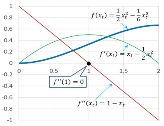
Figure 5.
Only under a very special circumstance could the second-order derivate at the mid-point of the constitutive curve be zero. In most cases, we still have .
Hence, the curve in the plane in Figure 4c must not go through the origin in a generic case. That is, the corresponding circuit element is active.
Furthermore, in Equation (8), we can deduce a formula for a third-order circuit element as below:
Observing Equations (8) and (11), we have a generic formula for a n-order circuit element as below:
where and is a polynomial function whose value is not equal to zero unless .
In order to examine whether the curve goes through the origin of the plane (that is the i-v plane for a memristor, the i-φ plane for an inductor, and the q-v plane for a capacitor, respectively), we let and examine the value of . Observing Equation (12) carefully, if the tested n-order element is locally passive, we must have and , …, for arbitrary nonzero excitations and . We have already proved that leads to , which is in contradiction to Criterion 2 (nonlinearity) for an ideal circuit element defined in Section 2. Thereby, we must have when , which implies that the tested higher-order element must be locally active.
The following activity theorem for a second-order or higher-order ideal memristor is therefore proven:
Theorem 2. (Local Activity Theorem).
A second-order or higher-order ideal memristor is locally active.
As can be seen in Section 7, this theorem is experimentally verified by the two active higher-integral-order memristors extracted from the Hodgkin-Huxley circuit [2,10,11].
4. A Second-Order Ideal Memristor Degenerates into a Negative Nonlinear Resistor: A Graphic Proof with a Sinusoidal Signal
So far, we have analytically verified the local activity of a second-order or higher-order ideal memristor with any possible shape of the excitation. In this section, we will use a graphic method based on the conformal differential transformation [5] to verify the above analytically verified local activity of a higher-order memristor. In scientific research, it is a common practice for a theorem to be established using different or complementary techniques and methods in terms of double-checking (or multi-checking) the conclusion independently.
An exemplified sinusoidal excitation will be conveniently used to draw a sample graph. Rigorously, this graphic approach is inadequate since the passivity of a circuit element refers to any possible shape of the excitation, as originally defined by Chua [13,15,16]. Nevertheless, this graphic proof complements the analytical proof in Section 3. The former provides a strict, generic proof for any possible shape of the excitation, whereas the latter visually and vividly depicts the local activity under a sinusoidal excitation as an example.
Beyond the first-order setting, second-order circuit elements require double-time integrals of voltage and current, namely, and . With the use of these additional variables [6], we may accommodate a second-order memristor and its nonlinear counterparts.
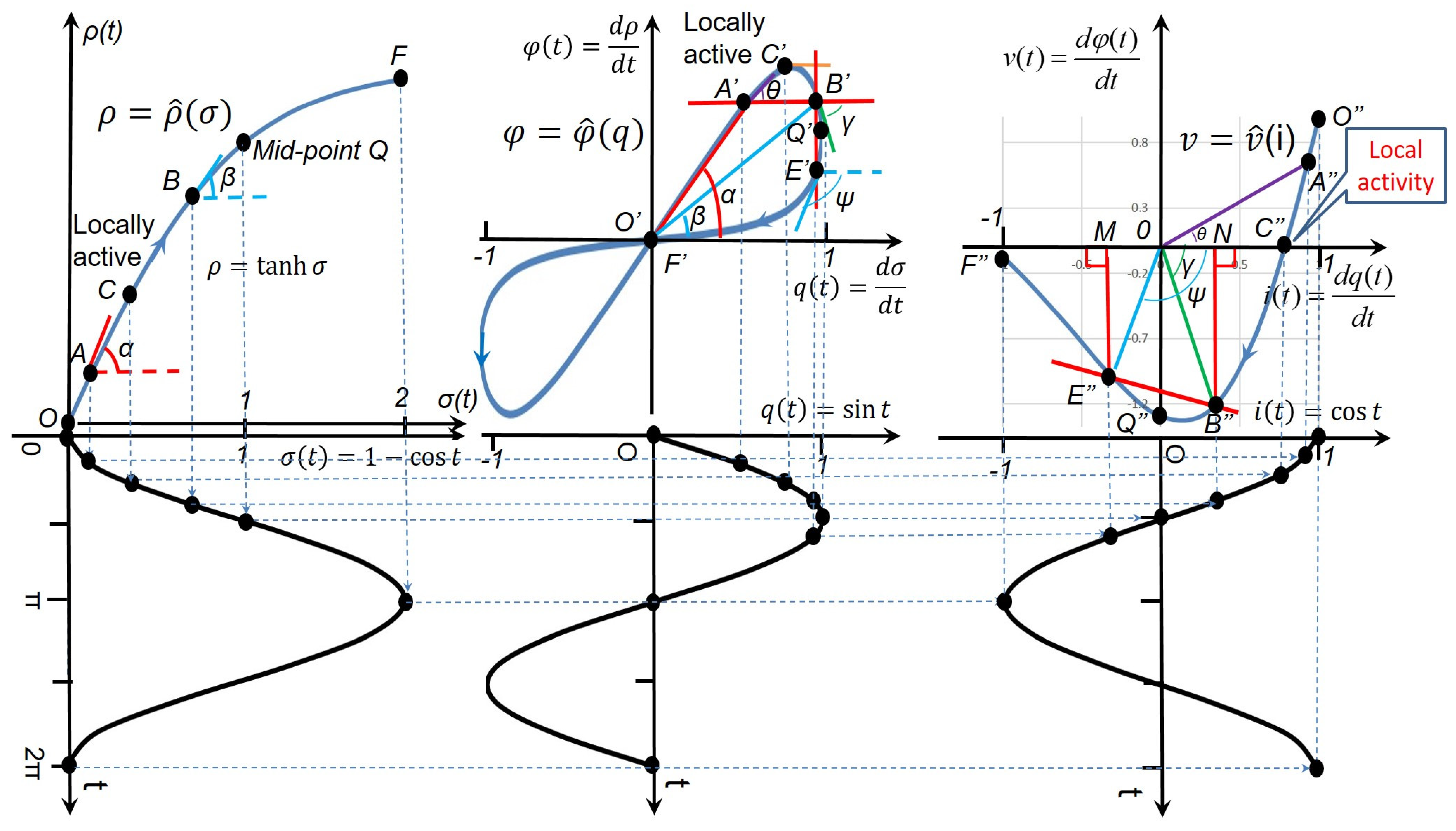
In the same way to define a first-order ideal memristor in Section 2, a second-order ideal memristor should be characterized by a time-invariant ρ-σ curve (Figure 6) complying with the same set of four criteria (as well as the same zero initial states) as mentioned in Section 2.
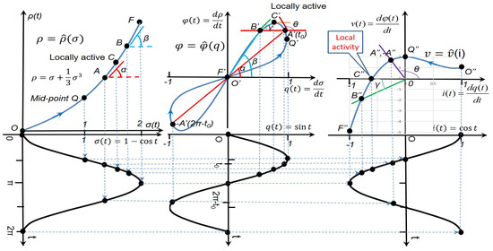
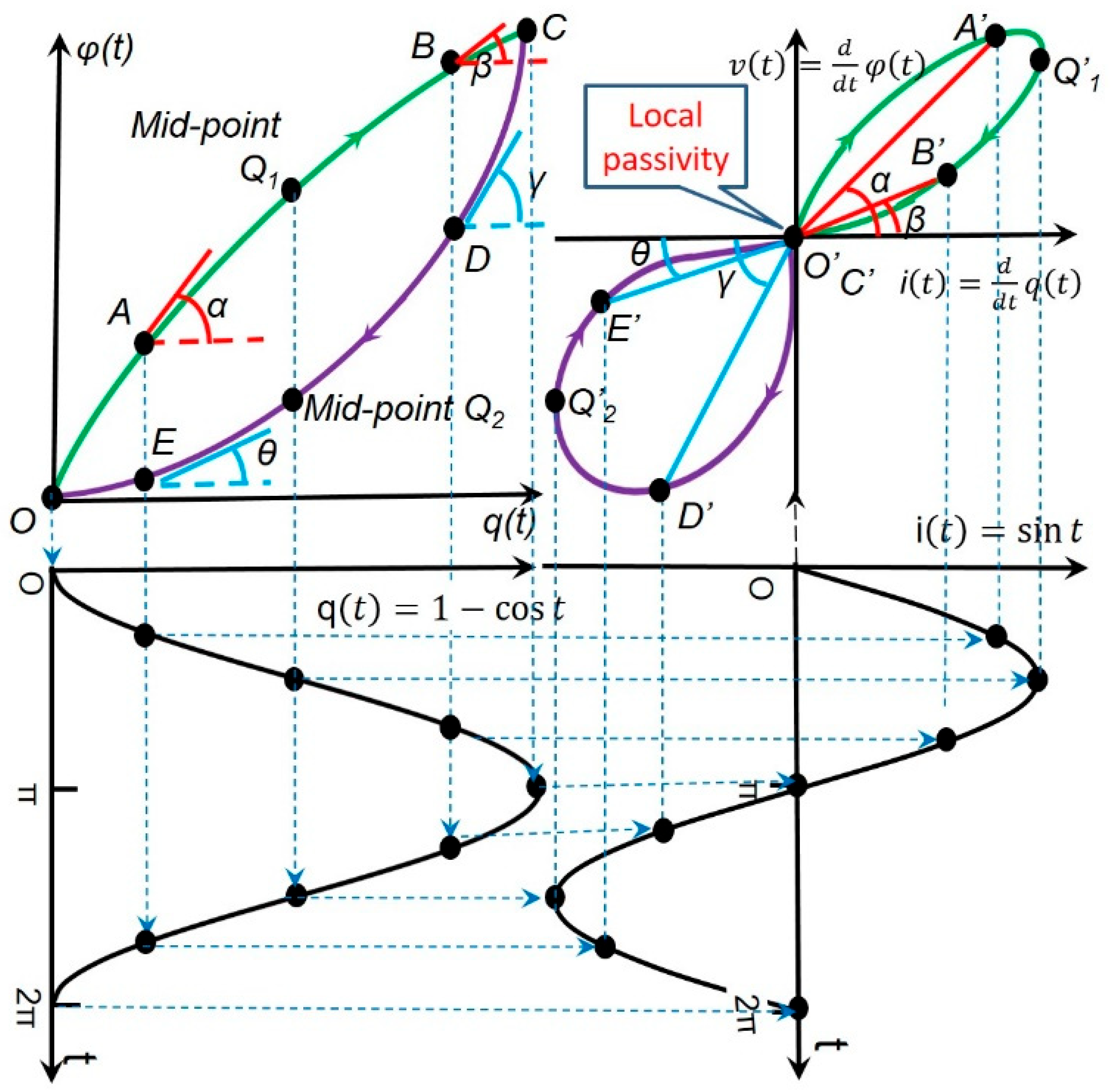
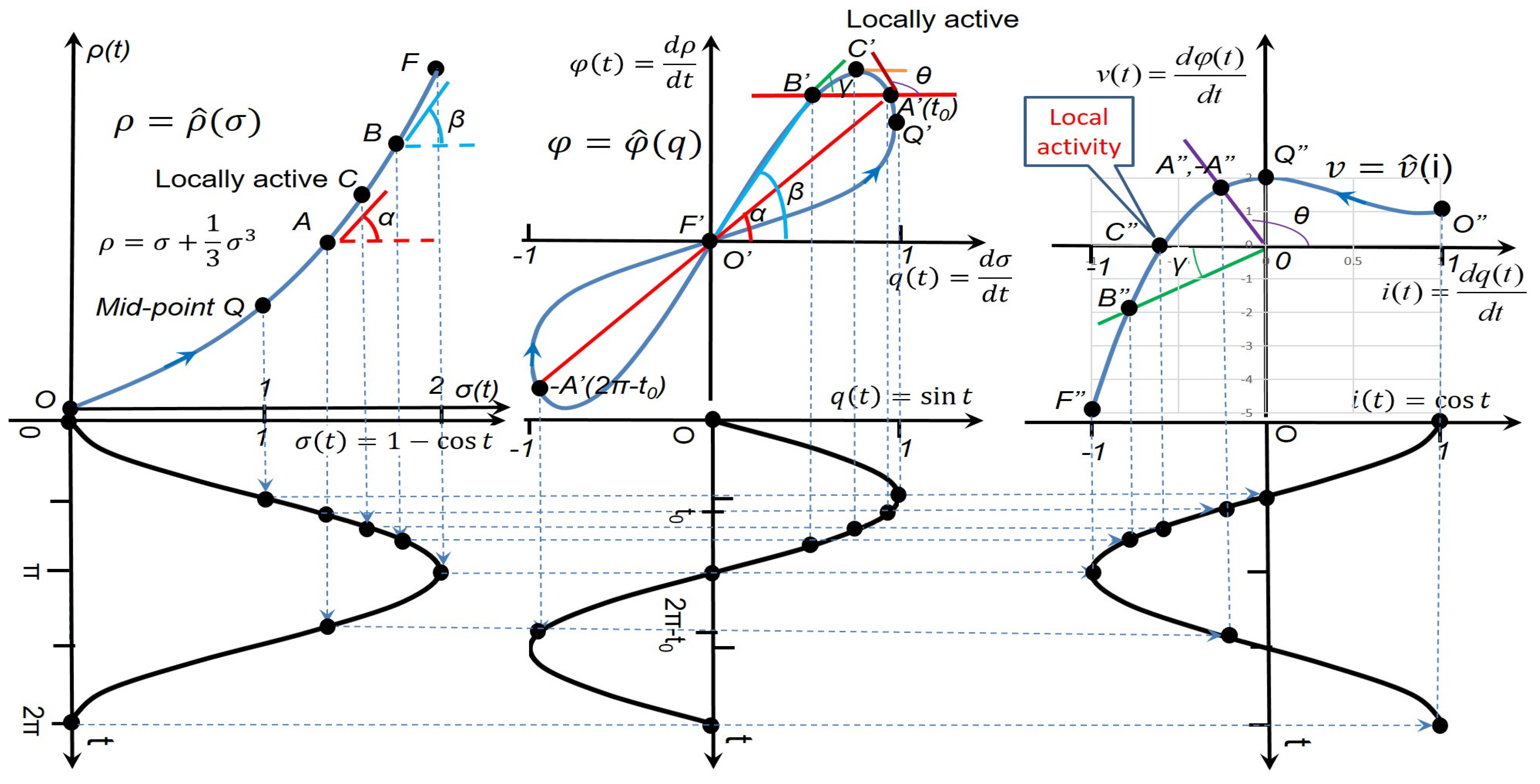
Figure 6.
A second-order ideal memristor requires double-time integrals of voltage and current, namely, σ = ∫qdt = ∬idt and ρ = ∫φdt = ∬vdt, as its constitutive attributes [6]. The constitutive ρ-σ curve should be time-invariant, single-valued, nonlinear, differentiable, and monotonically increasing to ensure its ideality. Two consecutive conformal differential transformations are required to generate a v-i locus that exhibits local activity and manifests itself as a negative nonlinear resistor with an internal power source. A″ denotes A’s projected point after two transformations. A polynomial is used here as an example to draw this graph.
With the aid of the aforementioned conformal differential transformation, a curve in the constitutive ρ-σ plane is transformed into a zero-crossing, double-valued Lissajous figure in the φ-q plane. As shown in Figure 6, following the O-Q-A-B-F path during the first half cycle (0 ≤ t ≤ π) in the ρ-σ plane, the chord (a straight line connecting a point to the origin) sweeps in a counterclockwise direction in the O′-Q′-A′-B′-F′ order in the first quadrant of the φ-q plane and then repeats the sweep in an asymmetric manner in the third quadrant during the second half cycle (π ≤ t ≤ 2π), resulting in an anti-symmetric pinched hysteresis loop . Because the ρ-σ curve is single-valued, the outgoing path (0 ≤ t ≤ π) overlaps the returning path (π ≤ t ≤ 2π) in and the corresponding pinched Lissajous figure is anti-symmetric with respect to the origin of the φ-q plane.
Consequently, another conformal differential transformation is performed, resulting in the slope (θ) of the line tangent to the curve at an operating point A′(t = t0) in the φ-q plane being equal to the same slope (θ) of a straight line connecting the projected point A″(t = t0) to the origin in the v-i plane. Because the φ-q curve is anti-symmetric with respect to its mid-point of the operating range (in this case, it is the origin), the corresponding v-i locus is single-valued, as shown in Figure 6.
The mathematical proof for being a single-valued function is as follows.
By the definition of anti-symmetry [f(−y, −x) = −f(x, y)] and q(t0) = sin t0 = −sin(2π − t0) = −q(2π − t0), i(t0) = cos t0 = cos(2π − t0) = i(2π − t0), we have
for a pair of points A′(t0) and −A′(2π − t0) that are anti-symmetric against the mid-point of the φ-q loop (overlapping the origin of the φ-q plane in Figure 6). We then obtain
and
The above two anti-symmetric points A′(t0) and –A′(2π − t0) in the φ-q plane are projected onto the v-i plane as one single point A″(−A″); therefore, the loci collapse into another single-valued function without passing through the origin. The above deduction can be summarized as follows:
Theorem 3. (Single-Value Theorem).
A single-valued function becomes another single-valued function after two consecutive conformal differential transformations.
It is easy to prove that this theorem is generic for any possible shape of the excitation, although Figure 6 is exemplified with a sinusoidal signal.
The circuit element with such a single-valued v-i curve (as shown in Figure 6) that does not go through the origin manifests itself as a nonlinear negative resistor [5], in which there must be an internal power source (either a current source or a voltage source). On the other hand, this single-value theorem ensures the zeroth-order of a negative nonlinear resistor, into which a second-order memristor degenerates.
An examination of the loci in Figure 6 reveals that this pinched hysteresis loop contains a small region (e.g., the short arc C′A′Q′) with a negative slope, which results in the projected points A″ being located in the second quadrant of the v-i plane. This observation also leads to the same conclusion that a second-order ideal memristor is locally active at the origin.
The mathematical proof of passivity is as follows.
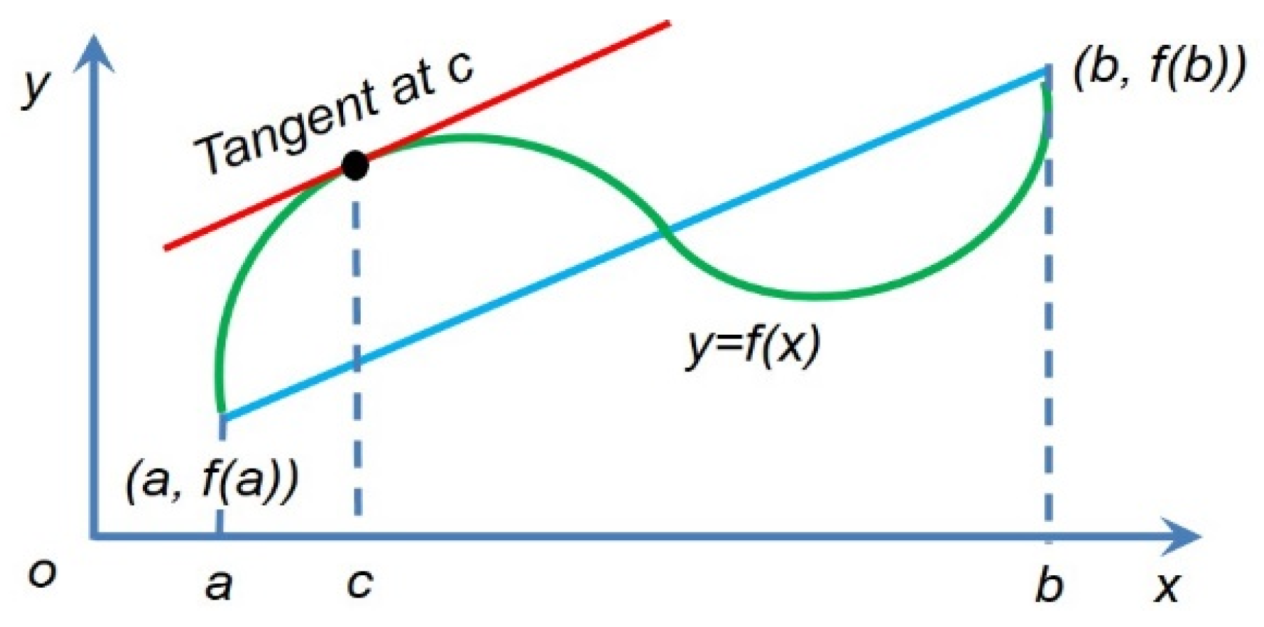
As shown in Figure 7, the mean value theorem [21] in mathematics states that if f is continuous on the closed interval [a, b] and differentiable on the open interval (a, b), then there must be a point c in (a, b) such that the tangent at c is parallel to the secant line joining the end-points (a, f(a)) and (b, f(b)); that is
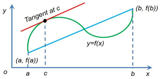
Figure 7.
Cauchy’s mean value theorem [21]. For any function that is continuous and differentiable, a point c on (a,b) must exist such that the secant joining the end-points of [a,b] is parallel to the tangent at c.
Now, let us go back to Figure 6. As proved in Section 2, the curve is a pinched Lissajous figure. Therefore, we can draw a horizontal secant to have two intersecting points A′ and B′ with the loop, as shown in Figure 6. According to the mean value theorem, a point C′ in (A′, B′) must exist such that the tangent at C′ is zero. With the aid of the second conformal differential transformation, C′ is projected onto the v-i plane as C″, which is located on the i axis and apart from the origin (). This is typically local activity [13,15,16].
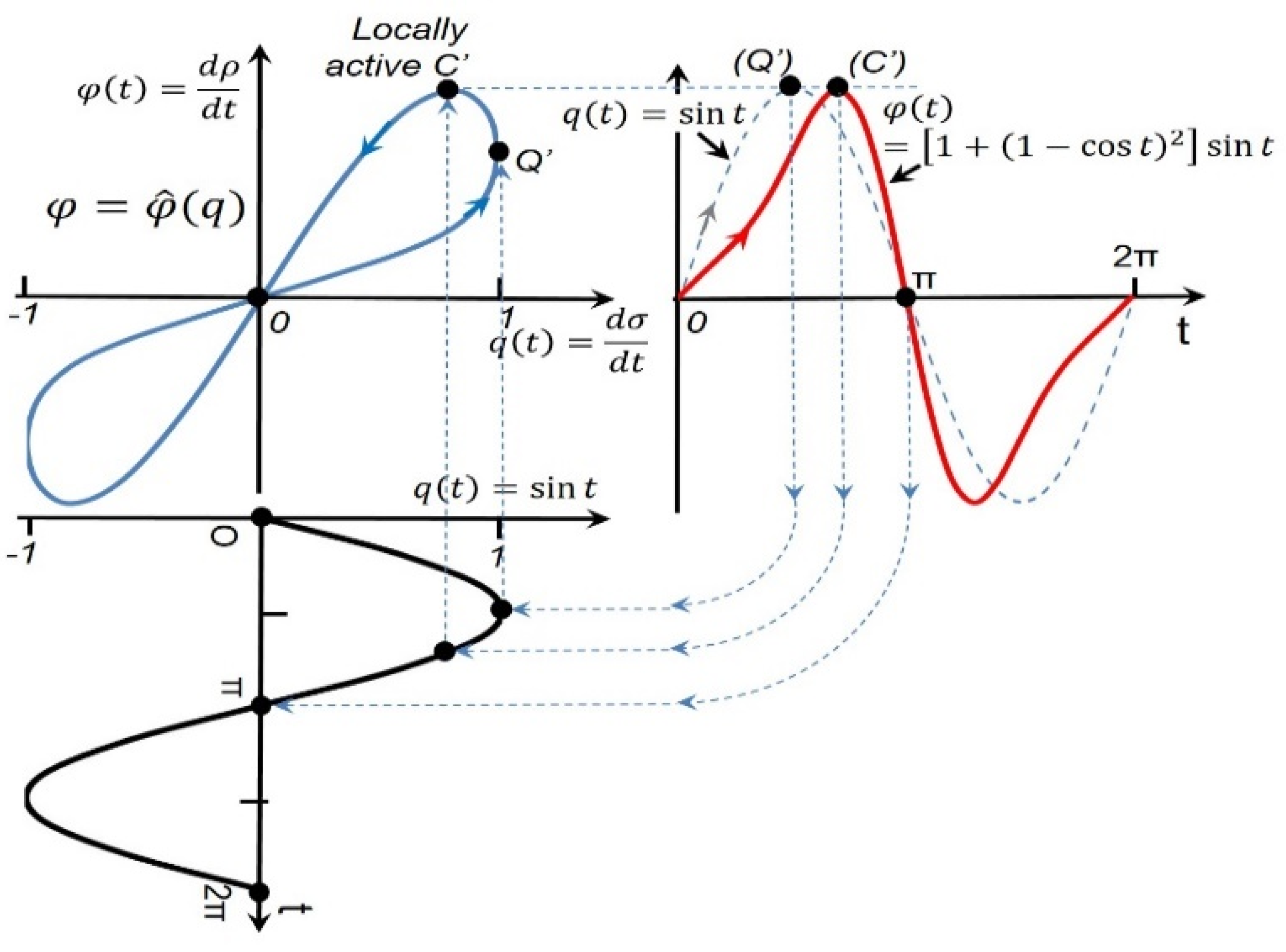
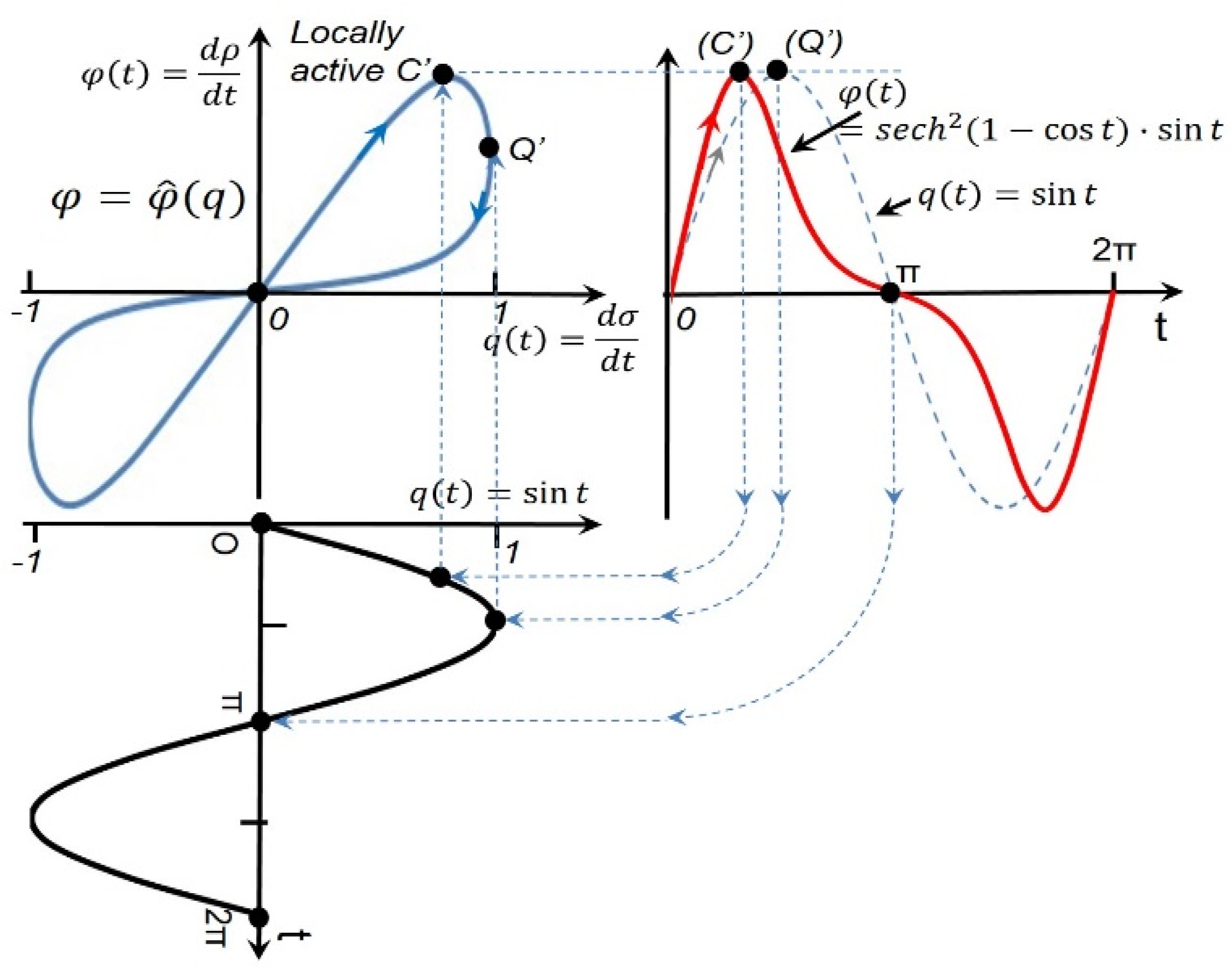
Point C′ exhibits local activity clearly. The origination of C′ in Figure 6 is illustrated in Figure 8, which corresponds to a maxima () of φ(t). The phase lag between the peak of the φ(t) waveform and the peak of the q(t) waveform can be clearly seen in this figure, which generates a small region (Q′, C′) with a negative slope in the φ-q plane. The end-point Q′ is projected from the mid-point Q of the constitutive ρ-σ curve as shown in Figure 6.

Figure 8.
The local activity point C’ in Figure 6 [] is originated from the peak of φ(t), which lags behind the peak of q(t), generating a small region (Q’, C’) with a negative slope. Since we obtain To facilitate the phase comparison, the height of the dashed q(t) waveform is scaled up to be aligned with that of φ(t).
Figure 6 and Figure 8 show an exemplified polynomial , which is the same as that used in Chua’s tutorial [5,8]. To a certain extent, this type of polynomial with unbounded slopes means “uncontrolled inflation” between the two variables, which may imply that an internal power source is always needed to support such an “unnatural” behavior, i.e., an internal power source is able to move C″ in Figure 9 to the origin (see Section 7 for details). Figure 9 uses a logistic function , which represents another type of “self-limiting” constitutive relation. is a logistic function [22,23]: . For values of x from −∞ to +∞, the S-curve shown in Figure 9, with the graph of f approaching 1 as x approaches +∞ and approaching zero as x approaches −∞.
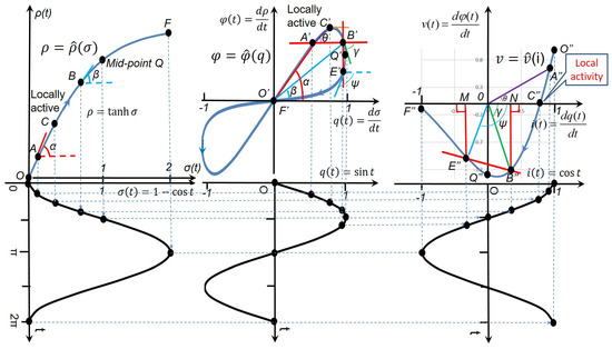
Figure 9.
A logistic function is used to draw the graph for a second-order ideal memristor, representing another type of constitutive relation in terms of self-limiting. Local activity can also be seen after two conformal differential transformations in this case, and this second-order memristor still degenerates into a negative nonlinear resistor with an internal power source.
The logistic function used in Figure 9 vividly depicts a self-limiting interaction between ρ and σ in a circuit element, where ρ responds to σ sensitively at the beginning and the saturation of ρ occurs while σ approaches +∞. We remark that self-limiting logistic q-φ curves were well observed in magnetic cores that are typically passive without any internal power source [24,25,26].
In contrast, Figure 9 exhibits local activity at the origin since the projected point C″ is located on the i axis and apart from the origin (). There must be an internal current source.
A similar examination of the loci in Figure 9 reveals that the pinched hysteresis loop contains a small region (e.g., the short arc C′B′Q′) with a negative slope, which results in the projected points B″ being located in the fourth quadrant of the v-i plane. This observation also leads to the same conclusion that a second-order ideal memristor is locally active.
The origination of C′ in Figure 9 () is illustrated in Figure 10, which corresponds to a maxima (dφ/dt = 0) of φ(t). The phase advance between the peak of the φ(t) waveform and the peak of the q(t) waveform can be clearly seen in this figure, which generates a small region (C′, Q′) with a negative slope in the φ-q plane.

Figure 10.
The local activity point C′ in Figure 9 [] is originated from the peak of φ(t), which leads the peak of q(t), generating a small region (C′, Q′) with a negative slope. Since we obtain . To facilitate the phase comparison, the height of the dashed q(t) waveform is scaled up to be aligned with that of φ(t).
A careful comparison of Figure 8 and Figure 10 reveals that the concave-convex orientation of the constitutive relation (as displayed in Figure 6 and Figure 9) plays two roles. On the one hand, it determines the winding direction of the loop; on the other hand, the former () causes a phase-lag between φ(t) and q(t) [accordingly, the local activity point is located in the second half of the constitutive curve], whereas the latter () causes a phase-advance [accordingly, the local activity point is located in the first half of the constitutive curve].
An even-higher-order memristor (α ≤ −3, β ≤ −3) can be studied by relaying a sequence of conformal differential transformations from the second-order memristor. As shown in Figure 9, a pair of consecutive points B′ and E′ in the φ-q plane (E′ leads B′) are projected onto the v-i plane as B″ and E″ that are subject to the same amplitude of an excitement current i. The height B″M of the laggard point B″ is found to be even lower than the height E″N of the leading point E″ as . The existence of such a pair of points obviously violates the fourth criterion (strictly monotonically increasing) of the ideality stated in Section 2. This trajectory makes it impossible for a third-order memristor to be ideal, in which another transformation is needed, in addition to the two transformations shown in Figure 9, to further project a v-i curve with a mixture of monotonically increasing and decreasing regions onto a sub-v-i plane. Intuitively, even if a single-valued, monotonically increasing constitutive curve cannot guarantee a passive v-i curve for a third-order memristor, an even-higher-order circuit element should exhibit a v-i behavior that is more complex than that exhibited in a nonlinear negative resistor with an internal power source [5].
5. A Higher-Order Ideal Mem-Inductor Is Locally Active
In the same way, to define a second-order ideal memristor in Section 3 and Section 4, a second-order ideal mem-inductor should be characterized by a time-invariant ∫ρ-σ curve complying with the same set of four criteria (as well as the same zero initial states) as mentioned above.
Intuitively, after the first conformal differential transformation from the original ∫ρ-σ plane, the curve is a pinched Lissajous figure. Similarly, we can draw a horizontal secant to intersect the loop at the two intersecting points A’ and B’. According to the mean value theorem [21], a point C′ in (A′, B′) must exist such that the tangent at C′ is zero. After the second conformal differential transformation, C′ is projected onto the φ-i plane as C″. This projected point C″ is located on the i axis and apart from the origin (), which indicates that there exists an internal current source; hence, a second-order mem-inductor is locally active.
By repeating the analytical proof with the two general constitutive variables (x, y) in Section 3, the following activity theorem (generic for any possible shape of the excitation) for a second-order or higher-order mem-inductor can be proven:
Theorem 4. (Local Activity Theorem).
A second-order or higher-order ideal mem-inductor is locally active.
It is worth mentioning that we used a computational amplifier and built an active inductor with memory to track an ameba’s time constant () in an adaptive neuromorphic architecture.
6. A Higher-Order Ideal Mem-Capacitor Is Locally Active
In the same way to define a second-order ideal memristor in Section 3 and Section 4, a second-order ideal mem-capacitor should be characterized by a time-invariant ρ-∫σ curve complying with the same set of four criteria (as well as the same zero initial states) as mentioned above.
Intuitively, after the first conformal differential transformation from the original ρ-∫σ plane, the curve is a pinched Lissajous figure. In contrast, we now draw a vertical secant to intersect the loop at the two intersecting points A′ and B′. According to the mean value theorem [21], there must exist a point Q′ in (A′, B′) such that the tangent at Q′ is . After the second conformal differential transformation, Q′ is projected onto the v-q plane as Q″. This projected point Q″ is located on the v axis and apart from the origin (), which indicates that there exists an internal voltage source; hence, a second-order mem-capacitor is locally active.
By repeating the analytical proof with the two general constitutive variables (x, y) in Section 3, the following activity theorem (generic for any possible shape of the excitation) for a second-order or higher-order mem-capacitor can be proven:
Theorem 5. (Local Activity Theorem).
A second-order or higher-order ideal mem-capacitor is locally active.
Both passive and active mem-capacitive systems were studied, in which the energy added to/removed from the system was found to be associated with some internal degree of freedom (some physical elastic or inelastic processes accompanying the change in conductance) [7].
7. Experimental Verification
We stress that the studied periodic table is for the ideal circuit elements with a single state variable [1]. However, in reality, most real-world circuit elements [24,25,26] are not ideal but have additional state variables, and they are called a broad class, such as memristive systems [2]. Hence, it is worth clarifying the relationship between an ideal circuit element (normally in theory) and those real devices (in practice) belonging to the same family led by that ideal circuit element. Without having direct relevance to the technical content of this study, an analog in chemistry is that Mendeleev predicted the existence of the (pure, ideal) chemical elements in his periodic table of chemical elements [17,27], and other chemists kept claiming they had found those predicted elements one by one in spite of their purities being less than 100% in the real world.
In 1971, to link the flux φ and the charge q, Chua predicted an ideal memristor with a single state variable that is either q or φ [1] after resistor [28], capacitor [29], and inductor [29]. Thirty-seven years later, HP announced that “The missing memristor found” [30]. As a real device, the HP memristor is not related to q or φ in an ideal way, as its state variable is the width “w” of the active TiO2 domain [30]. However, since the active TiO2 domain is doped with positively charged ions, the width "w" is still a function of the charge q as shown below [30]:
where is average ion mobility, is (low) resistance of a region with a high concentration of dopants (positive ions) that can drift under an external bias v(t), and D is the full length of the HP memristor. Separated by the boundary (moved by v), the two regions include the above-mentioned one with and the other with a low dopant concentration and much higher resistance [30].
In Equation (16), the state variable of the HP memristor can still be viewed as q (but with a “purity” of less than 100%). Despite its non-ideality, the HP memristor is still recognized as the first physical (first-order) memristor since it exhibits the distinctive zero-crossing fingerprint or signature [2], i.e., it is passive (without being constructed from active components). The (memory) resistance of the HP memristor is [30] as follows:
which squares with the form for the first-order memristor defined by Chua [1,2].
Similar to the above physical HP memristor [30], the second-(state-)order sodium memristor in the Hodgkin-Huxley circuit is not ideal, as its two (independent) state variables are the ionic gate-activation probability m and the ionic gate-inactivation probability h, respectively [2,10,11], rather than the (pure) charge q. The sodium ion-channel memductance function is a two-variable fourth-order polynomial (mentioned in Section 4) as shown below:
where [11]. However, these two state variables are still related to q (but with a “purity” of less than 100% due to the approximation to be performed) because those positively charged ions are present. If we approximate that and , we can rewrite Equation (18) as follows:
which squares with the generic form for charge-controlled third-integral-order memristive systems [2]. Notice that the state order [that is the number of internal state variables [12] (i.e., m, h, )] and the integral order (that is in in Figure 1) should not be mixed up here.
The first-(state-)order potassium memristor in the Hodgkin-Huxley circuit is not ideal either, as its single state variable is the ionic gate-activation probability n [2,10,11] rather than the (pure) charge q. The potassium ion-channel memductance function is a one-variable fourth-order polynomial as shown below:
where [11]. Similar to the above two sodium state variables, this potassium state variable is also related to q with a “purity” of less than 100%. If we approximate that , we can rewrite Equation (20) as follows:
which squares with the generic form for charge-controlled fourth-(differential)-order memristive systems [2].
Therefore, by the same standard well-used in the evolutionary history of the circuit theory, our claim that all the higher-order (≥2) circuit elements must be active was experimentally verified by the second-(state-)order [that is equivalent to the third-integral-order in this example] sodium memristor that is locally active with an internal battery () [10,11] and the first-(state-)order [that is equivalent to the fourth-integral-order in this example] potassium memristor that is locally active with an internal battery () [10,11].
As mentioned in Section 4, a polynomial function has unbounded slopes, which may imply that an internal power source is always needed to support such an “unnatural” behavior. Further research is needed.
8. Conclusions, Discussions, and Future Work
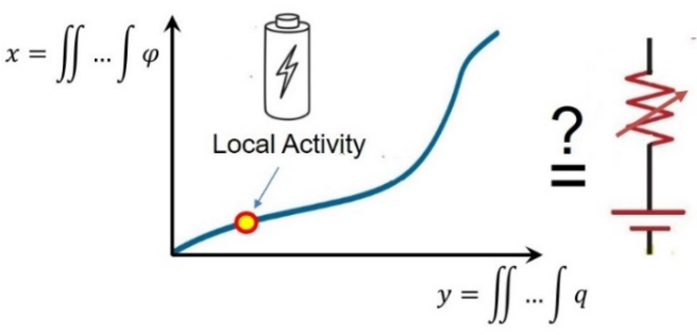
As shown in Figure 11, our study can be simplified to an open question in circuit theory:

Figure 11.
An open question in circuit theory: Is a single-valued, nonlinear, continuously differentiable, and monotonically increasing constitutive curve x-y locally active? Our theorems show that there must be at least one local active operating point on the curve.
Is a single-valued, nonlinear, continuously differentiable, and monotonically increasing constitutive curve locally active?
Based on an analytical proof with any possible shape of the excitation and a graphical proof with a sinusoidal excitation, our finding is that all higher-order passive memory circuit elements [memristor (α ≤ −2, β ≤ −2), higher-order inductor (α ≤ −3, β ≤ −2), and higher-order capacitor (α ≤ −2, β ≤ −3)] must have an internal power source; hence, their passive versions do not exist in nature since they are bound to degenerate into zeroth-order negative nonlinear elements with an internal power source, as shown in Figure 11. Their active versions (with either an electric, optical, chemical, nuclear, or biological power source) may still be found in nature (e.g., the two higher-integral-order memristors in the Hodgkin-Huxley circuit [2,10,11]) or may be built as an artifact in the lab with the aid of active components (e.g., transistors or operational amplifiers) and power supplies.
Our claim that all the higher-order (≥2) circuit elements must be active was experimentally verified by the two active higher-integral-order memristors extracted from the Hodgkin-Huxley circuit [10,11]. The value of our study is that if one asks why we have never seen any passive higher-order (≥2) circuit elements over the past 200 years since Ohm discovered the resistance and developed Ohm’s Law in 1827 [28], they may find an answer from our paper.
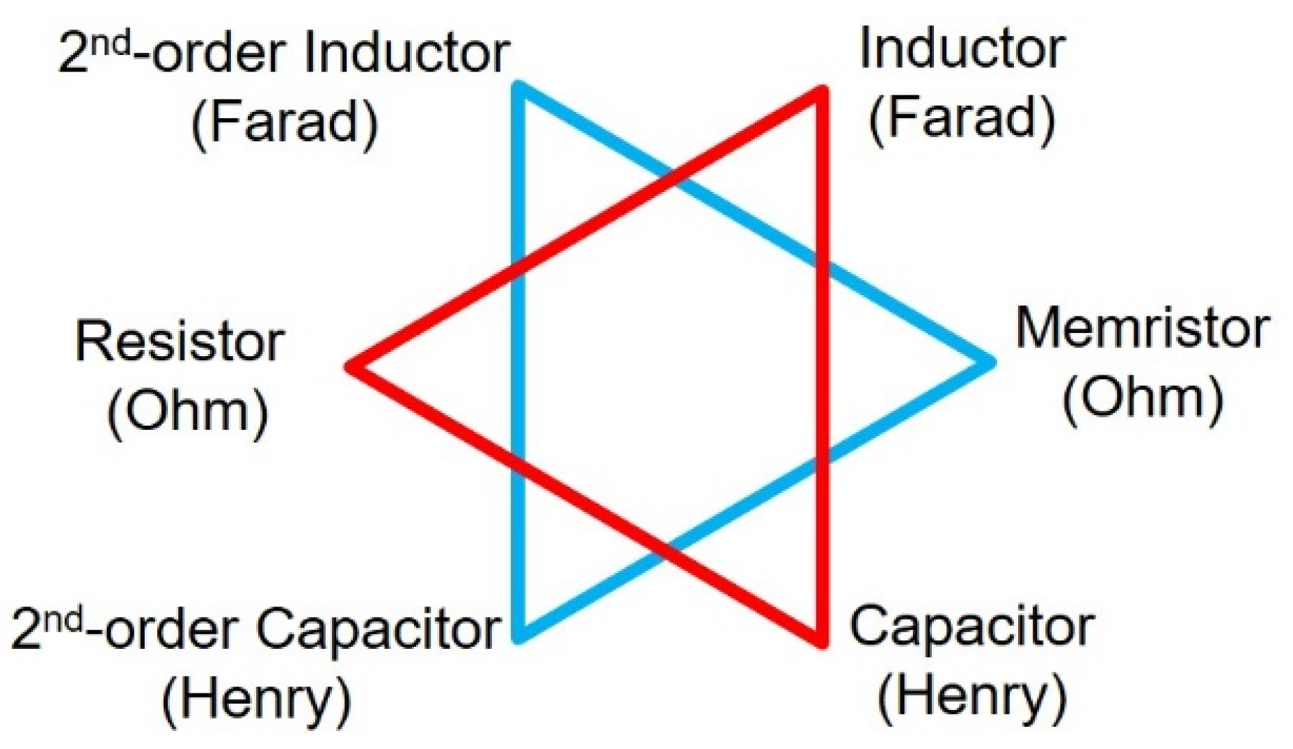
Consequently, the periodic table of the two-terminal passive ideal circuit elements can be dramatically reduced to a reduced table comprising only six passive ideal elements: a resistor, inductor, capacitor, memristor, mem-inductor, and mem-capacitor, as shown in Figure 12. Such a bounded table is believed to be concise, mathematically sound, and aesthetically symmetric, which may mark the finish of the hunt for missing higher-order (passive) circuit elements predicted by Chua in 1982 [3]. To date, all six elements in this reduced table have been fully studied: resistors [28], inductors [29], capacitors [29], memristors [1,2,30], mem-inductors [5,8,31,32], and mem-capacitors [5,8].
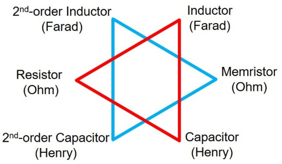
Figure 12.
A six-pointed star of all passive ideal circuit elements. It is composed of a pair of face-to-face equilateral triangles, with their intersection as a regular hexagon. The first triangle includes the three traditional ideal circuit elements (resistor, capacitor, and inductor), whereas the second triangle includes the three new but argumentative ideal circuit elements since Chua called his predicted memristor a fourth circuit element [1,5]. The units in the diagram highlight the correspondence between the two triangles. This new table is a big leap from an infinity in Chua’s table (Figure 1) to a bound of six circuit elements only.
Based on the fractional calculus [33,34,35,36,37], the table can be extended to include more fraction-order circuit elements in addition to the six (integer-order) passive ideal circuit elements: the intermediate case between the apexes (the integer-order circuit elements) represents fractional circuit elements, in which the interaction between the two constitutive attributes is fractional [36].
In this paper, we have studied the passivity [13,15,16] of those () circuit elements defined by Chua in his periodic table [32,38]. It is, therefore, natural for us to use the ideal memristor in Chua’s 1971/2003/2011 definition for the ideal circuit elements [1,5,8] rather than their 1976 definition for “a broad generalization of memristors (memristive systems)”. We remark that our work has nothing to do with the memristive systems due to no periodicity.
Notwithstanding the fact that chemistry is a dramatically different scientific area from circuits and systems, however, our study was originally motivated by Mendeleev’s periodic table of chemical elements, in which chemical elements beyond uranium (with atomic number 92) were not found in nature because they were too unstable, and all chemical elements with a higher atomic number than 118 remain purely hypothetical [17]. We will study whether Chua’s predicted higher-order passive circuit element candidates on the three diagonals in his periodic table [3] exist, which may be our new contributions to the circuit theory domain.
As an analog in Mendeleev’s periodic table of pure chemical elements [27] (rather than chemical compounds consisting of atoms of two or more chemical elements), it is impossible to work out a periodic table of non-ideal circuit elements, such as memristive systems, due to their non-existent periodicity and unpredictable complexity (whose states can be anything with any number). As a matter of fact, a periodic table of chemical compounds did not exist. At least in this work, our intention is to study the ideal circuit elements only, as highlighted in the title.
We remark that a correct circuit element table may request to rewrite the textbooks in electrical/electronic engineering and physics since a reduced table marks the end of the hunt for missing higher-order passive circuit elements predicted 40 years ago [3]. Its potential engineering applications are expected to bring about enormous changes in our everyday lives in terms of circuit elements being the building blocks of modern computers and electrical/electronic devices.
As an argumentative idea about the periodic table of circuit elements for future work, we will address “the case for rejecting the memristor as a fundamental circuit element” (the title of Abraham’s 2018 paper [39]), in which a unique perspective is presented in the sense that that the “charge” is the single fundamental electronic entity as well as its associated entity “voltage” (since the separation of the positive and negative charges builds up electrical potential energy and a non-zero voltage appears). “Magnetic flux” and “current” are not thought to be fundamental any longer since both entities are merely a result of various states of motion of the charge [36]. A charge/voltage-based periodic table was used to re-categorize the circuit elements, and it was found that the memristor had no entry in the table [39]. We will dispute this because the motion of the charge is not the only source to generate magnetic flux in all cases. As can be illustrated in our spin information storage work [39], magnetic flux may be caused by spontaneous magnetization or spin. Even if it is “internal molecular currents” that generate the magnetization, it must be different or independent of an (externally applied) current [39]. In our opinion [40], the flux (resulting from spontaneous magnetization or spin) is still fundamental (as universally acknowledged by the whole magnetics community), and so is the memristor that links the flux and the charge.
Normally, the active version of a circuit element has to be complex in its structures to accommodate an electric, optical, chemical, nuclear, or biological power source. An analog in chemistry is that chemical elements with a higher atomic number than 92 were not found in nature because they were too unstable and may decay radioactively into other chemical elements [17]. The passivity of the first-order memristor (that is the key element in our reduced periodic table of six passive ideal circuit elements) exhibits its indivisible structure and its fundamentalness in terms of linking the two fundamental physical attributes: the charge and the flux [32].
As another argumentative idea about the periodic table of circuit elements for future work, we will study whether the pinched-loop (Figure 2, Figure 3, Figure 4, Figure 5, Figure 6, Figure 7, Figure 8, Figure 9 and Figure 10, except Figure 7) can be used as signature behavior observable in one plane. In light of the findings reported in Ref. [31], obtaining this behavior is related to satisfying the phase and magnitude conditions of the theory of Lissajous figures, which necessitates a nonlinear device. Therefore, all these “higher-order” mem-devices boil down to the theory of Lissajous figures [41]. There is no memory in all of these “passive and nonlinear” devices because the memory is associated with the parasitic capacitors or inductors in the fabricated devices claiming to be “mem-devices” [42].
As concurrent work, topology can be used to show the topological features of these devices [43]. In science, claims must be demonstrated and validated experimentally. One reviewer is still concerned with the well-known references (namely, the HP memristor and the Hodgkin-Huxley circuit) with their limitations. In the future, we will be able to address these concerns if we obtain additional details. In another future work, we will study the passive or active nature of the real device when the signal under test has noise. Our theory is based on analytical proof with any possible shape of the excitation, which implies that, in principle, the proposed passivity criterion should have strong resilience to noises.
Funding
This research was partially funded by an EC grant “Re-discover a periodic table of elementary circuit elements”, PIIFGA2012332059, Marie Curie Fellow: Leon Chua (UC Berkeley), Scientist-in-charge: Frank Wang (University of Kent).
Data Availability Statement
All data generated and analyzed during this study are included in this published article.
Conflicts of Interest
The authors declare no conflicts of interest. The funders had no role in the design of the study; in the collection, analyses, or interpretation of data; in the writing of the manuscript; or in the decision to publish the results.
References
- Chua, L. Memristor—The Missing Circuit Element. IEEE Trans. Circuit Theory 1971, 18, 507–519. [Google Scholar] [CrossRef]
- Chua, L.; Kang, S. Memristive Devices and Systems. Proc. IEEE 1976, 64, 209–223. [Google Scholar] [CrossRef]
- Chua, L.; Szeto, E. High-Order Non-Linear Circuit Elements: Circuit-Theoretic Properties; UC Berkeley: Berkeley, CA, USA, 1982. [Google Scholar] [CrossRef]
- Chua, L.; Szeto, E. Synthesis of Higher Order Nonlinear Circuit Elements. IEEE Trans. Circuit Syst. 1984, 31, 231–235. [Google Scholar] [CrossRef]
- Chua, L. Nonlinear Circuit Foundations for Nanodevices. Part I: The Four-Element Torus. Proc. IEEE 2003, 91, 1830–1859. [Google Scholar] [CrossRef]
- Biolek, D.; Biolek, Z.; Biolkova, V. SPICE modeling of memristive, memcapacitive and meminductive systems. In Proceedings of the European Conference on Circuit Theory and Design, Antalya, Turkey, 23–27 August 2009; pp. 249–252. [Google Scholar]
- Pershin, Y.; Ventra, M.D.; Chua, L. Circuit Elements with Memory: Memristors, Memcapacitors, and Meminductors. 2009. Available online: https://arxiv.org/pdf/0901.3682.pdf (accessed on 4 July 2024).
- Chua, L. Resistance switching memories are memristors. Appl. Phys. A Mater. Sci. Process. 2011, 102, 765–783. [Google Scholar] [CrossRef]
- Georgiou, P.; Barahona, M.; Yaliraki, S.N.; Drakakis, E.M. On memristor ideality and reciprocity. Microelectron. J. 2014, 45, 1363–1371. [Google Scholar] [CrossRef]
- Chua, L.; Sbitnev, V.; Kim, H. Hodgkin-Huxley axon is made of memristors. Int. J. Bifurc. Chaos 2012, 22, 1230011(1)–1230011(48). [Google Scholar] [CrossRef]
- Sah, M.; Kim, H.; Chua, L. Brains Are Made of Memristors. IEEE Circuits Syst. Mag. 2014, 14, 12–36. [Google Scholar] [CrossRef]
- Riaza, R. Second order mem-circuits. Int. J. Circuit Theory Appl. 2015, 43, 1719–1742. Available online: https://mc.manuscriptcentral.com/ijcta (accessed on 4 July 2024). [CrossRef]
- Mainzer, K.; Chua, L. Local Activity Principle: The Cause of Complexity and Symmetry Breaking; Imperial College Press: London, UK, 2013. [Google Scholar]
- Biolek, Z.; Biolek, D.; Biolkova, V. Lagrangian for Circuits with Higher-Order Elements. Entropy 2019, 21, 1059. [Google Scholar] [CrossRef]
- Chua, L. Everything You Wish to Know About Memristors but Are Afraid to Ask. In Handbook of Memristor Networks; Springer: Berlin/Heidelberg, Germany, 2015. [Google Scholar]
- Corinto, F.; Forti, M.; Chua, L. Nonlinear Circuits and Systems with Memristors; Springer: Berlin/Heidelberg, Germany, 2021; ISBN 978-3-030-55650-1. [Google Scholar]
- Available online: https://en.wikipedia.org/wiki/Periodic_table (accessed on 4 July 2024).
- Vaidyanathan, S.; Volos, C. Advances in Memristors, Memristive Devices and Systems; Springer: Berlin/Heidelberg, Germany, 2017. [Google Scholar]
- Chua, L.; Sirakoulis, G.C.; Adamatzky, A. Handbook of Memristor Networks; Springer Nature: Berlin, Germany, 2019. [Google Scholar]
- Available online: https://en.wikipedia.org/wiki/Mathematical_proof (accessed on 4 July 2024).
- Cauchy Theorem, Encyclopedia of Mathematics; EMS Press: Helsinki, Finland, 2001.
- Available online: https://en.wikipedia.org/wiki/Self-limiting_(biology) (accessed on 4 July 2024).
- Abraham, I.; Ren, S.; Siferd, R.E. Logistic Function Based Memristor Model with Circuit Application. IEEE Access 2019, 7, 166451–166462. [Google Scholar] [CrossRef]
- Menyuk, N.; Goodenough, J. Magnetic materials for digital computer components. I. A theory of flux reversal in polycrystalline ferromagnetics. J. Appl. Phys. 1955, 26, 8–18. [Google Scholar] [CrossRef]
- Gyorgy, E.M. Rotational model of flux reversal in square loop ferritcs. J. Appl. Phys. 1957, 28, 1011–1015. [Google Scholar] [CrossRef]
- Cushman, N. Characterization of Magnetic Switch Cores. IRE Trans. Compon. Parts 1961, 8, 45–50. [Google Scholar] [CrossRef]
- Mendeleev, D. The Periodic Law of the Chemical Elements [Excerpted from Liebigs Annalen, 8th supplement (1871). pp. 133–239. Available online: https://web.lemoyne.edu/~giunta/Mendeleev1871.pdf (accessed on 4 July 2024).
- Ohm, G. Die Galvanische Kette, Mathematisch Bearbeitet; Bei T.H. Riemann: Berlin, Germany, 1827; Volume 250. [Google Scholar]
- Faraday, M. Experimental Researches in Electricity; Bernard Quaritch: London, UK, 1833. [Google Scholar]
- Strukov, D.; Snider, D.; Stewart, S.; Williams, S. The missing memristor found. Nature 2008, 453, 80–83. [Google Scholar] [CrossRef]
- Wang, F.Z.; Chua, L.O.; Yang, X.; Helian, N.; Tetzlaff, R.; Schmidt, T.; Li, L.; Carrasco, J.M.; Chen, W.; Chu, D. Adaptive Neuromorphic Architecture (ANA). Special Issue on Neuromorphic Engineering: From Neural Systems to Brain-Like Engineered Systems. Neural Netw. 2013, 45, 111–116. [Google Scholar] [CrossRef]
- Wang, F.Z. A Triangular Periodic Table of Elementary Circuit Elements. IEEE Trans. Circuits Syst. 2013, 60, 616–623. [Google Scholar] [CrossRef]
- Petras, I.; Chen, Y.; Coopmans, C. “Fractional-Order Memristive Systems. In Proceedings of the 14th IEEE International Conference on Emerging Technologies and Factory Automation, Mallorca, Spain, 22–26 September 2009. [Google Scholar] [CrossRef]
- Muñoz-Pacheco, J. Infinitely many hidden attractors in a new fractional-order chaotic system based on a fracmemristor. Eur. Phys. J. Spec. Top. 2019, 228, 2185–2196. [Google Scholar] [CrossRef]
- Jahanshahi, H.; Yousefpour, A.; Munoz-Pacheco, J.M.; Kacar, S.; Pham, V.T.; Alsaadi, F.E. A new fractional-order hyperchaotic memristor oscillator: Dynamic analysis, robust adaptive synchronization, and its application to voice encryption. Appl. Math. Comput. 2020, 383, 125310. [Google Scholar] [CrossRef]
- Wang, F.Z. Fractional memristor. Appl. Phys. Lett. 2017, 111, 243502. [Google Scholar] [CrossRef]
- Pu, Y.; Yuan, X. Fracmemristor: Fractional-order memristor. IEEE Access 2016, 4, 1872–1888. [Google Scholar] [CrossRef]
- Chua, L. If it’s pinched it’s a memristor. Semicond. Sci. Technol. 2014, 29, 104001. [Google Scholar] [CrossRef]
- Abraham, I. The case for rejecting the memristor as a fundamental circuit element. Nat. Sci. Rep. 2018, 8, 10972. [Google Scholar] [CrossRef]
- Wang, F.Z. Near-Landauer-Bound quantum computing using single spins. IEEE Trans. Quantum Eng. 2023, 4, 2100513. [Google Scholar] [CrossRef]
- Maundy, B.; Elwakil, A.S.; Psychalinos, C. Correlation Between the Theory of Lissajous Figures and the Generation of Pinched Hysteresis Loops in Nonlinear Circuits. IEEE Trans. Circuits Syst. I Regul. Pap. 2019, 66, 2606–2614. [Google Scholar] [CrossRef]
- Salaoru, I.; Li, Q.; Khiat, A.; Prodromakis, T. Coexistence of memory resistance and memory capacitance in TiO2 solid-state devices. Nanoscale Res. Lett. 2014, 9, 552. [Google Scholar] [CrossRef]
- Wang, F.Z. Topological electronics: From infinity to six. J. Comput. Electron. 2023, 22, 913–920. [Google Scholar] [CrossRef]
Disclaimer/Publisher’s Note: The statements, opinions and data contained in all publications are solely those of the individual author(s) and contributor(s) and not of MDPI and/or the editor(s). MDPI and/or the editor(s) disclaim responsibility for any injury to people or property resulting from any ideas, methods, instructions or products referred to in the content. |
© 2024 by the author. Licensee MDPI, Basel, Switzerland. This article is an open access article distributed under the terms and conditions of the Creative Commons Attribution (CC BY) license (https://creativecommons.org/licenses/by/4.0/).