Abstract
Time-sensitive networking (TSN) is considered an ideal solution to meet the transmission needs of existing industrial production methods. The traffic scheduling problem of TSN is an NP-hard problem. The traditional traffic scheduling algorithms can lead to issues such as significant computational time consumption and traffic congestion, which are not conducive to the rapid and high-quality deployment of TSN. To simplify the complexity of TSN schedule table generation, the paper studies the scheduling problem of mixed critical traffic in TSN. Using a combinatorial packing traffic scheduling algorithm based on unoccupied space (CPTSA-US), a scheduling table for TSN traffic transmission is generated, proving the feasibility of transforming the TSN traffic scheduling problem into a packing problem. In addition, the initial packing algorithm and traditional traffic scheduling algorithm can cause traffic accumulation, seriously affecting network performance. This paper proposes a mixed-critical traffic scheduling algorithm based on free time domain (MCTSA-FTD), which further partitions the packing space transformed by the time domain. And performs multiple packing of traffic based on the partitioned packing space and generates the TSN schedule table according to the reverse transformation of the packing results. The simulation results show that compared to the CPTSA-US and the traditional traffic scheduling solution algorithm SMT (Satisfiability Modulo Theory), the schedule table generated by the MCTSA-FTD significantly improves the delay, jitter, and packet loss of BE flows in the network while ensuring the transmission requirements of TT flows. This can effectively enhance the transmission performance of the network.
1. Introduction
1.1. Background
With the vigorous rise of the new round of technological revolution and industrial transformation, the surge in video traffic and industrial machine applications has brought about a large amount of congestion control and data packet delay. However, many industries require end-to-end latency to be controlled within microseconds to milliseconds. For example, the autonomous driving system in automobiles requires the end-to-end latency of the onboard network to be within 250 us, and the electronic control system inside the car requires it to be less than 10 us. In addition to latency requirements, these applications also demand microsecond-level jitter control and extremely low packet loss rates. However, traditional Ethernet can only reduce the end-to-end latency to tens of milliseconds, and it lacks deterministic transmission mechanisms, thus only providing best-effort transmission services. It cannot meet the “on-time, accurate” transmission requirements of critical data traffic in the new industrial ecosystem [1].
So far, existing research has proposed a series of effective solutions with each solution targeting specific field requirements. For example, there are protocols such as Controller Area Network (CAN) [2] primarily focusing on the automotive fields; Time-Triggered Ethernet (TTEthernet) [3]; the Avionics Full-Duplex Switched Ethernet (AFDX) [4] for the avionics fields; and Fieldbus systems like SERCOS III [5], EtherCAT [6], and PROFINET [7] for the industrial fields. However, these solutions either lack mutual compatibility or cannot be integrated with standard Ethernet devices, resulting in issues such as application incompatibility, poor interoperability, difficulty in portability, and high development, deployment, and operational maintenance costs. As Industry 4.0 and the new round of industrial revolution strongly stimulate the informatization and digitalization of industrial control, the demand for “one network fits all” is becoming increasingly prominent.
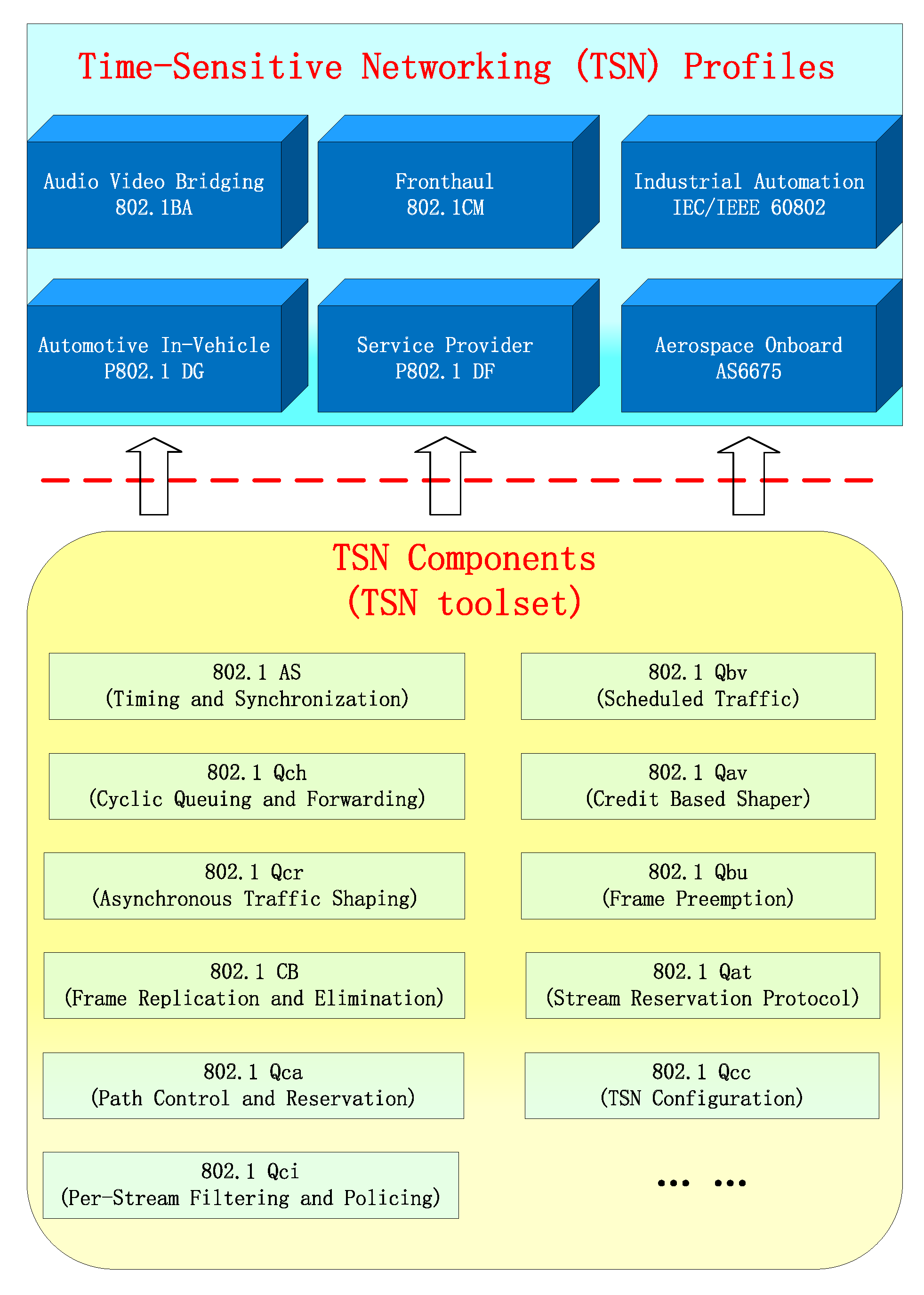
In order to meet the transmission requirements of critical data traffic in the new industrial ecosystem for “on-time, accurate” delivery, promote the development of standardized industrial Ethernet, and overcome the low bandwidth and compatibility issues of existing bus-type networks, the Time-Sensitive Networking (TSN) working group was established. The group has proposed a series of standards and specifications for link layer enhancements and traffic management strategies, including time synchronization [8], traffic scheduling [9,10,11], reliable transmission [12], and network management [13], to extend standard Ethernet into TSN. The TSN standards are mainly modifications and extensions of the 802.1Q standard [14], with each modification forming a substandard. Currently, the maturity level of TSN technical standards is relatively high, and standards and specifications for TSN in six major vertical industries are being developed. Figure 1 illustrates the TSN application scenarios and their common technologies.
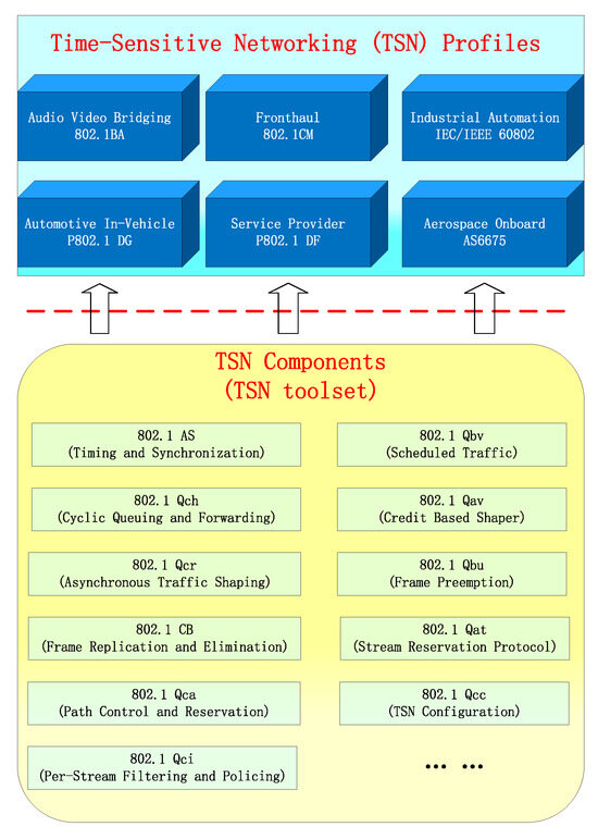
Figure 1.
TSN standards for the six major application scenarios and their common technologies.
TSN ensures deterministic latency at the physical and link layers in different scenarios by selecting different TSN components, effectively meeting the real-time communication transmission requirements of modern industrial production methods, and providing a reliable and efficient network communication infrastructure for industrial control systems.
TSN classifies the transmission of data into three categories based on different flow requirements [15]. (1) Time-Triggered (TT) flows have the highest priority in traffic transmission. They are transmitted in a preemptive manner, and the transmission timing of these messages is predictable. (2) Audio-Video Bridge (AVB) flows are mainly bursty flows with certain latency requirements Due to the burstiness of the data, traffic shapers are used to smooth the transmission and ensure the upper bound of the AVB flow’s latency. (3) Best-effort (BE) flows are primarily flows with no specific latency requirements and are transmitted using the best-effort (BE) transmission method in Ethernet, which has no time constraints. TSN traffic scheduling refers to the use of specific scheduling algorithms to determine the transmission order and timing of each data frame across all switch egress ports. This ensures that each data frame can smoothly pass through all egress ports along the transmission path in the entire network while meeting the latency and bandwidth requirements of different types of traffic. This allows different types of traffic to coexist on the same network and achieve low latency and reliable transmission for critical data streams [16,17].
In practical analysis and computation, the scheduling problem of TSN presents significant complexity due to the diversity of network structures and variations in data flows and their quality of service. Numerous studies have shown that traffic scheduling in TSN is an NP-complete problem, and its difficulty in solving is related to the number of variables and constraints. Therefore, as the network topology becomes more complex and the number of flows increases, the scheduling difficulty increasesred [18]. Inefficient and highly complex scheduling algorithms can result in significant computational time consumption, traffic congestion, and other related issues, which are detrimental to the rapid and high-quality deployment of TSN, severely impacting the overall performance of TSN networks.
1.2. Related Works
After understanding the scheduling issue of TSN traffic transmission, we need to solve this problem and obtain a traffic transmission scheme. Then, we map this scheme to the Gate Control List (GCL) to achieve the transmission of TSN traffic [19]. Traditional TSN traffic scheduling mechanisms can be classified into five categories based on the solution methods adopted: Integer Linear Programming (ILP), heuristic algorithm (HA), Satisfiability Modulo Theory (SMT), Tabu Search (TS) and Greedy Randomized Adaptive Search Procedure (GRASP). Ref. [20] proposes the objective function as the weighted sum of minimizing the number of queues occupied by TT flows and the distance between end-to-end latency and its lower bound. It formalizes the traffic scheduling problem as a multi-objective combinatorial optimization problem and uses an ILP solver to find the scheduling solution. However, due to the scalability issues of ILP, it is only suitable for seeking optimal solutions in small-scale networks. Ref. [21] presents a heuristic scheduling method based on genetic algorithms for event-triggered messages in time-sensitive networks. This method improves the system’s schedulability, message transmission efficiency, and resource utilization but significantly increases the complexity of the algorithm. Ref. [22] proposes a low-complexity algorithm based on ant colony optimization to solve the online routing problem of AVB traffic in TSN networks. However, there is a heavy scheduling problem during the routing process. Therefore, heuristic algorithms cannot obtain optimal solutions and cannot guarantee the quality of the solutions. Refs. [23,24] propose a traffic-type allocation and joint scheduling mechanism based on TS. Pop et al. design a scheduling mechanism based on GRASP [25]. Both TS and GRASP are metaheuristic algorithms that guide the search for optimal solutions in the solution space. They differ in the initial solution generation and neighborhood search algorithms. TS and GRASP are suitable for large-scale networks with a smaller search space, but the quality of the obtained solutions is generally average. Steiner et al. propose a series of traffic scheduling schemes based on the SMT [26,27,28]. Ref. [29] applies SMT calculation to allocate time windows that satisfy scheduling constraints at each output port in the network. After traversing all output ports, a global scheduling scheme is formed, which greatly reduces the computational overhead compared to global SMT solving. However, the computational overhead of the SMT-based scheduling table generation method remains significant when dealing with large-scale networks and high loads.
Ref. [30] explores the potential application of packing problems and scheduling problems. Ref. [31] applies traditional packing algorithms to the scheduling of time-triggered messages in Time-Triggered Ethernet (TTE) and improves and optimizes them. Building on the combination of packing problems and TTE scheduling, Ref. [32] proposes an Improved Finite Horizontal Algorithm (IFH) suitable for TTE scheduling problems, and it has been proven that the packing algorithm for TTE traffic scheduling has a smaller computational time consumption compared to traditional TTE traffic scheduling algorithms. Furthermore, packing problems benefit from mature algorithms and optimization techniques that can be applied to address slot allocation and traffic scheduling optimization in TSN (Time-Sensitive Networking). This can be likened to the packing problem where items of different sizes need to be placed into boxes of limited capacity to maximize space utilization and avoid overlap or waste during the packing process. Common packing algorithms such as First Fit, Best Fit, and Worst Fit can be utilized for slot allocation optimization in TSN traffic scheduling, aiming to maximize network bandwidth utilization and reduce the probability of slot conflicts.By referencing the application of packing algorithms in TTE and considering the NP-completeness of traffic scheduling problems in TSN and the optimization characteristics of packing problems, the time-triggered scheduling problem in TSN is transformed into a packing problem. The transformation can effectively resolve the issue of traffic congestion in TSN caused by time-triggered flows, thereby improving the transmission service for other types of traffic. This helps facilitate the rapid and high-quality deployment of TSN.
1.3. Contributions
The main contributions of this paper are summarized as follows:
(1) The paper presents the TSN switch architecture and the mixed-critical traffic scheduling model. According to the periodical characteristic of the TT traffic, the mixed-critical traffic scheduling problem in TSN is transformed into a two-dimensional packing problem, and the scheduling constraints are provided.
(2) A two-dimensional packing algorithm suitable for solving TSN time-triggered scheduling, called the combination packing traffic scheduling algorithm based on unoccupied space (CPTSA-US), is presented. Using this algorithm combined with the inverse transformation of packing results, we generated a TSN traffic scheduling table. This validation demonstrates the feasibility of transforming the mixed-critical traffic scheduling problem in TSN into a two-dimensional packing problem and has initially alleviated the congestion issues of Time-Triggered (TT) traffic.
(3) We propose a mixed-critical traffic scheduling algorithm based on free time domain (MCTSA-FTD). It addresses the issue of traffic accumulation when packing algorithms are directly applied to TSN mixed-critical traffic scheduling. The scheduling table generated by the proposed algorithm is then simulated. The analysis shows that the MCTSA-FTD can evenly Improving the transmission performance of Best Effort (BE) flows while not affecting the transmission performance of TT flows.
The remaining parts of this paper are as follows. Section 2 starts with the network architecture, TSN switch structure, and traffic scheduling model, introducing the system model of traditional TSN traffic scheduling problems. Section 3 transforms the TSN traffic scheduling problem into a two-dimensional packing problem and discusses the constraints of using packing algorithms for TSN traffic scheduling. Section 4 describes the proposed CPTSA-US and MCTSA-FTD algorithms in detail. In Section 5, performance analysis and comparison of the traffic in TSN are conducted for the scheduling tables generated by the two algorithms. Finally, Section 6 provides a summary of the entire paper. Section 7 provides a detailed description of future research directions.
2. System Model
2.1. Network Architecture Model
The TSN network architecture is represented by an undirected topology graph where ( and are sets representing the end systems and switches in the network, respectively) represents the set of all nodes in the network, and E represents the set of all physical links in the network. The vertex represents a node in the architecture, which can be either an end system () or a network switch (). The edge represents a physical link between node and node , and all physical links in the network are full-duplex links. Figure 2 presents a simple TSN network architecture with four switches and nine end systems.
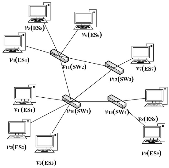
Figure 2.
An architecture model example: include five TSN switches () and nine end systems (). The represents the physical link from vertex to vertex .
The link between two physical devices defines a data link in two directions. In this paper, the set of data links is denoted as L. The data link between adjacent nodes and is represented as , where . It should be noted that and are two different data links. The set of communication links from end-to-end systems is denoted as . The communication link from end system to end system is represented as , where . For a redundant network topology, there may be multiple communication links between end systems. For example, in Figure 2, there are multiple communication links between nodes and . One option could be , while another option could be . In practical transmission, if there are multiple communication links available for transmitting traffic from one end system to another, various factors need to be considered in order to select the appropriate communication link for flows [33].
2.2. TSN Switch Architecture
Time-Aware Shaper (TAS) [10] is the core mechanism for achieving the deterministic real-time transmission of TT flows in TSN, which is standardized as 802.1 Qbvred [11]. TAS utilizes Gate Control Lists (GCLs) to accurately reserve bandwidth for TT flows [34]. However, due to the uncertainty of BE flows, it is possible that TT flows are being transmitted when a BE begins its transmission. To avoid conflicts between TT flows and BE, 802.1 Qbv defines the Protected Band strategy to achieve the deterministic transmission of TT flows [35]. However, this strategy may result in bandwidth waste.
To reduce the impact of low-priority frames on high-priority transmission, the IEEE 802.1Qbu standard defines the Frame Preemption strategy [36,37]. However, this strategy cannot preempt low-priority frames with a frame length smaller than 123 bytes, as the minimum frame length defined by standard Ethernet is 64 bytes. This delay of high-priority frames by 123 bytes will occur. When cascading multiple switches, the delay of high-priority frames will accumulate linearly. Therefore, this strategy cannot be directly applied to preempt BE with TT, as it will significantly weaken the determinism of TT transmission.
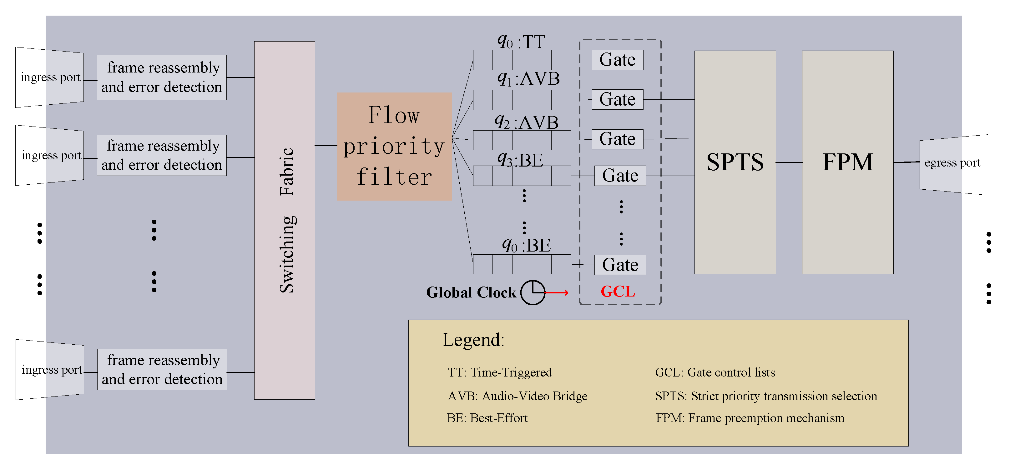
In the paper, a single-node TSN traffic scheduling algorithm is adopted, which needs to consider the transmission time of a TT flow in the previous node when generating its transmission time in a certain node. The deterministic requirement for TT transmission is high. Additionally, since the algorithm in this paper evenly distributes TT flows on the time axis, the conflict domain between TT and BE flows is greatly increased. Therefore, a hybrid strategy combining Protected Band and Frame Preemption is employed in the paper. The size of the Protected Band, denoted as , is set to 123 bytes, and the Frame Preemption strategy is executed moments before the start of TT traffic transmission. This strategy effectively avoids conflicts between TT and BE flows, ensures the determinism of TT traffic transmission, and minimizes bandwidth loss in the Protected Band. The structure of a TSN switch using the hybrid strategy is shown in Figure 3.
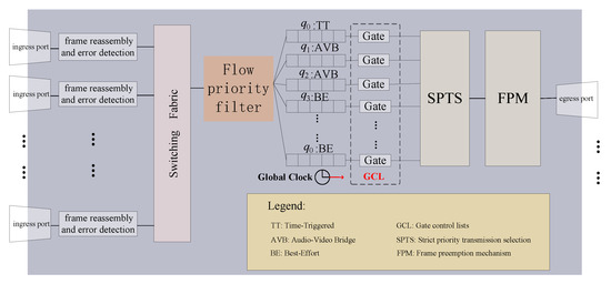
Figure 3.
Structure diagram of TSN switch with mixed frame preemption and Protected Band mechanism.
2.3. Mixed-Criticality Traffic Model
To accurately describe the behavior of flows in the network, the set of all flows is denoted as F, and the ith flow is denoted as (). The parameters of each flow are defined as follows:
where is the flow identifier of the flow; and , respectively, represent the source node and destination node of the flow; is the sending period of the flow from the source vertex to the destination vertex, represents the generation time of the flow; indicates the length of the data frame of the flow, which is measured in bytes; is the deadline of the flow, which means the difference between the receiving time at the destination node and the sending time at the source node should be within the deadline.
For any flow , i.e., ∀, if its and remain constant over time, such flow is referred to as a Time-Triggered (TT) flow. TSN achieves the deterministic transmission of TT by precisely specifying the transmission time point for each TT flows through Time-Triggered scheduling.
If a flow has a period and length that are not constant but functions of time t, then this flow is referred to as a Best-Effort (BE) flow. The BE flows model can characterize various types of Ethernet traffic, such as sporadic BE models with a constant and following a certain probability distribution. is the period time function of the traffic identified as i. It can also model BE for audio and video transmission, where can be a joint distribution of multiple probability distributions, and takes discrete values representing different BE levels. Due to the complexity of practical application scenarios, TSN does not set a specific transmission method for a particular application scenario but adopts a unified traffic shaper and priority scheduling to ensure the quality of service for BE flows.
In TSN traffic transmission, the end-to-end latency of TT flows depends on the transmission time points specified by the scheduling in the switches. Additionally, TSN strictly prioritizes traffic transmission, where BE flows are transmitted during the intervals of TT flows, and their performance is influenced by the distribution of the TT timeline. Therefore, in TSN traffic transmission, it is necessary to schedule TT flows first. While ensuring the schedulability of multiple TT flows, adjustments to the transmission intervals of TT flows are needed to optimize the end-to-end latency of BE flows.
3. Mixed-Critical Traffic Scheduling Problem Based on Combinatorial Packing
3.1. Transformation of Flow Scheduling Problem
The essence of TSN flow scheduling is how to arrange TT flows reasonably in the communication time domain of TSN, so that TT can be transmitted without conflict, with periodicity and determinacy according to the scheduled arrangement in the network. Under the premise of meeting the performance requirements of TT flows, the transmission performance of BE flows can be satisfied as much as possible. The essence of the packing problem is to purposefully place the items to be packed in the packing space so as to achieve the expected goal. Therefore, the two have a common essence, and it is feasible to transform the TT scheduling in TSN into packing scheduling: that is, to complete the transformation from TT to items to be packed and from time-domain resources to packing space.
In TSN networks, TT flows are known in advance, and numerous TT flows each have different periods and frame lengths. In order to schedule all infinite cyclic TT flows, it is necessary to define a finite length scheduling timetable as the transmission unit for all TT flows. This timetable is the least common multiple of all the TT flows’ periods, which is referred to as the super-period and denoted by . Therefore, it is only necessary to study the sending nodes of TT flows within a super-period and then cyclically transmit data according to the scheduling table in units of the super-period. Within one super-period, all TT messages complete at least one cycle. Therefore, the size of the super-period can be regarded as the packing space of the packing problem. By introducing the concept of a minimum period, whose size is the greatest common divisor of all the TT flows’ periods, referred to as the basic period denoted by , within one basic period, the same flow can transmit at most once. Then, the time resources of length are folded according to to complete the transformation from time-domain resources to two-dimensional packing space with the height () and width () as shown in Equations (1) and (2):
The transformation process is illustrated in Figure 4.
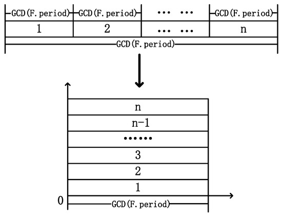
Figure 4.
Time-domain resource transformation diagram.
The width of the box is related to the rate at which nodes transmit data to the link in the network. Here, it is assumed that all nodes in the network have the same data transmission rate to the link (, in units of byte/ms). According to the transformation of time-domain resources, the generated two-dimensional packing space has the horizontal axis representing the number of bytes transmitted per unit time and the vertical axis representing the period time, which correspond exactly to the and of TT flows, respectively. Therefore, TT flows can be transformed into a two-dimensional packing item with a height and width as shown in Equations (3) and (4):
3.2. Scheduling Constraints
In order to ensure the determinism and real-time performance of TT flows, TSN provides services such as collision-free transmission and highest-priority service for TT flows to ensure the transmission performance of TT messages. In addition, certain latency requirements for BE flows need to be met. Therefore, when generating the scheduling table, constraints need to be imposed on the scheduling of TT flows to ensure the implementation of the aforementioned services. The following are some constraints that must be satisfied during the scheduling process:
- (1).
- Collision-free transmission constraints for TT flows.
In TSN, flows are transmitted over the link using TDMA. The generation of the scheduling table must avoid any two TT flows appearing on the same link at the same time, and the TT flow on a link must be strictly transmitted in accordance with the order of the scheduling table. The subsequent TT data frame must begin transmission only after the previous data frame has completed its transmission. This constraint can be expressed as shown in Equation (5):
where () represents the time node when node sends data to node for the k (t) th occurrence of TT flow ().
- (2).
- Path sequence constraints for flows.
For any flow , when it is transmitted over the adjacent paths and , it is always received by node first and then forwarded from . This constraint is expressed as shown in Equation (6):
where represents the transmission processing time at node , represents the propagation delay on data link , and represents the protection interval between flows.
- (3).
- End-to-end latency constraints.
In order to ensure the real-time performance of TT flows in TSN, strict deadlines must be defined for each TT flow to enforce end-to-end latency requirements. This constraint is expressed as shown in Equation (7):
where represents the acceptance time point of the kth arrival of the TT data frame with identifier at the destination vertex, and represents the kth arrival of the TT data frame with identifier at the sending node of the source vertex.
In addition, for AVB flows, the end-to-end latency is also required to be within a certain range. This constraint is expressed as shown in Equation (8):
where represents the transmission delay of the AVB flow identified as , and represents the deadline of the AVB flow identified as .
- (4).
- Simultaneous forwarding constraints for multicast flows.
This constraint describes a multicast flow , where it is constrained to be simultaneously transmitted to multiple links when it is multicast from node to multiple links. This constraint is specifically represented as shown in Equation (9):
where () represents the time node when node sends data to node () for the kth occurrence of multicast flows .
- (5).
- Network bandwidth constraints.
According to TSN, TT flows have strict requirements for frame length and end-to-end latency. Therefore, TSN must provide sufficient bandwidth; otherwise, if the transmission delay becomes too long, it may result in exceeding the latency and transmission failure. The required bandwidth for a TT flow is given by
where represents the minimum bandwidth required for the TT flow identified as .
For a BE flow with latency requirements, assuming TSN sets the maximum allowable latency for this type of flows as , the required bandwidth guarantee is given by
where represents the minimum bandwidth required for the BE flow with latency requirements identified as .
4. TSN Mixed-Criticality Traffic Scheduling Algorithm
4.1. Flows (Items) Preprocessing Phase
Since the physical links used in TSN support full-duplex communication, both receiving and sending can be simultaneously transmitted. Additionally, for flows with non-overlapping virtual links, synchronous transmission is possible. In a redundant network topology, there are multiple end-to-end communication links, resulting in multiple choices for the transmission virtual links of flows. Therefore, this paper designs a traffic preprocessing phase before the packing algorithm, which integrates flows based on virtual links and selects suitable transmission virtual links for each flow. The set of transmission virtual links for flows is denoted as . For each flow’s transmission virtual links, there is only one.
Suppose we have two flows, and , and their transmission virtual links are represented as shown in Equations (12) and (13):
If all L in are not equal to L in , then and can be transmitted synchronously, which means that these two flows are not interfered with during the packing process. After the traffic preprocessing phase, all flows have a determined virtual transmission path, and data that cannot be synchronously transmitted in a single node are integrated for the next step of the packing algorithm phase.
4.2. Combinatorial Packing Traffic Scheduling Algorithm Based on Unoccupied Space (CPTSA-US)
The packing problem is a combinatorial optimization problem that involves boxes and items to be packed. Based on the dimensions of the target variables, it can be divided into one-dimensional packing, two-dimensional packing, three-dimensional packing, and high-dimensional packing. From the previous problem transformation, it can be seen that the packing problem in TSN’s traffic scheduling mainly considers two attributes, which belong to the two-dimensional packing problem.
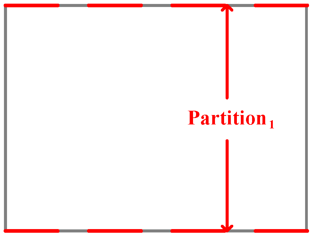
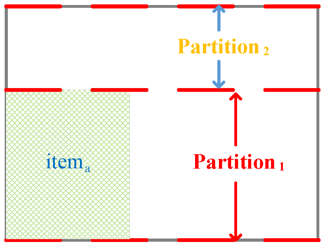
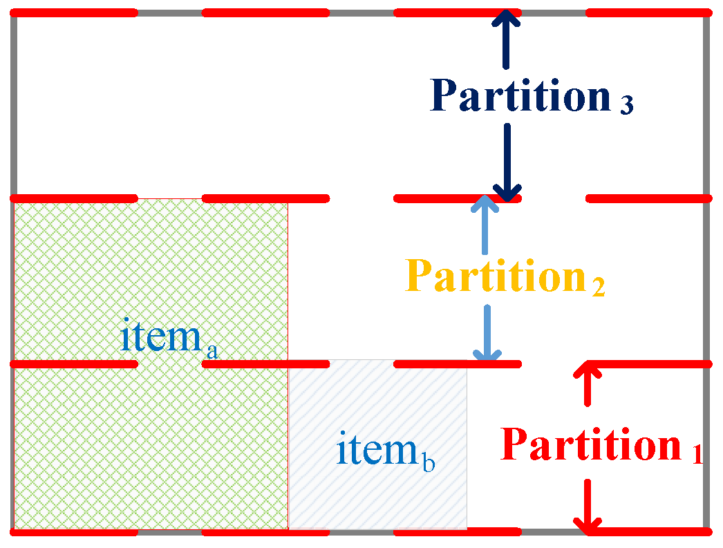
In this paper, a two-dimensional packing algorithm scheduling TT flows is proposed, the combinatorial packing traffic scheduling algorithm based on unoccupied space (CPTSA-US). The approach defines a vector with a size of , where each element represents the unoccupied width for each row. represents the current unoccupied space in the packing area. As shown in Figure 5, when the packing space is empty, all elements in are . The box is then partitioned based on the changes in elements. Based on the judgment of whether can be placed in the box, if it can, item a is placed in the lower-left corner of the partition, and the sizes of the elements in are updated. The partitioning is then adjusted based on the changes in elements, as shown in Figure 6. Similarly, when placing , the partitioning is adjusted accordingly, as shown in Figure 7. Since the height of the partition decreases from large to small, items need to be packed in descending order of height during the packing process.
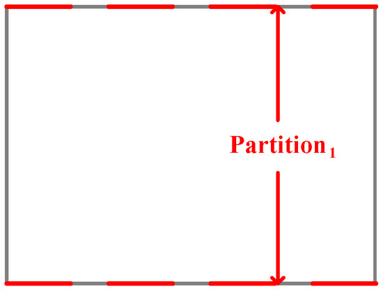
Figure 5.
Packing status when the packing space is empty.
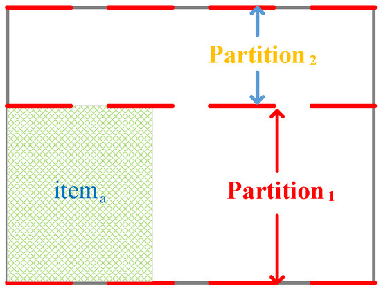
Figure 6.
Packing status after placing .

Figure 7.
Packing status after placing .
The algorithm process of the CPTSA-US is shown in Algorithm 1.
| Algorithm 1 Combinatorial Packing Traffic Scheduling Algorithm Based on Unoccupied Space (CPTSA-US) |
|
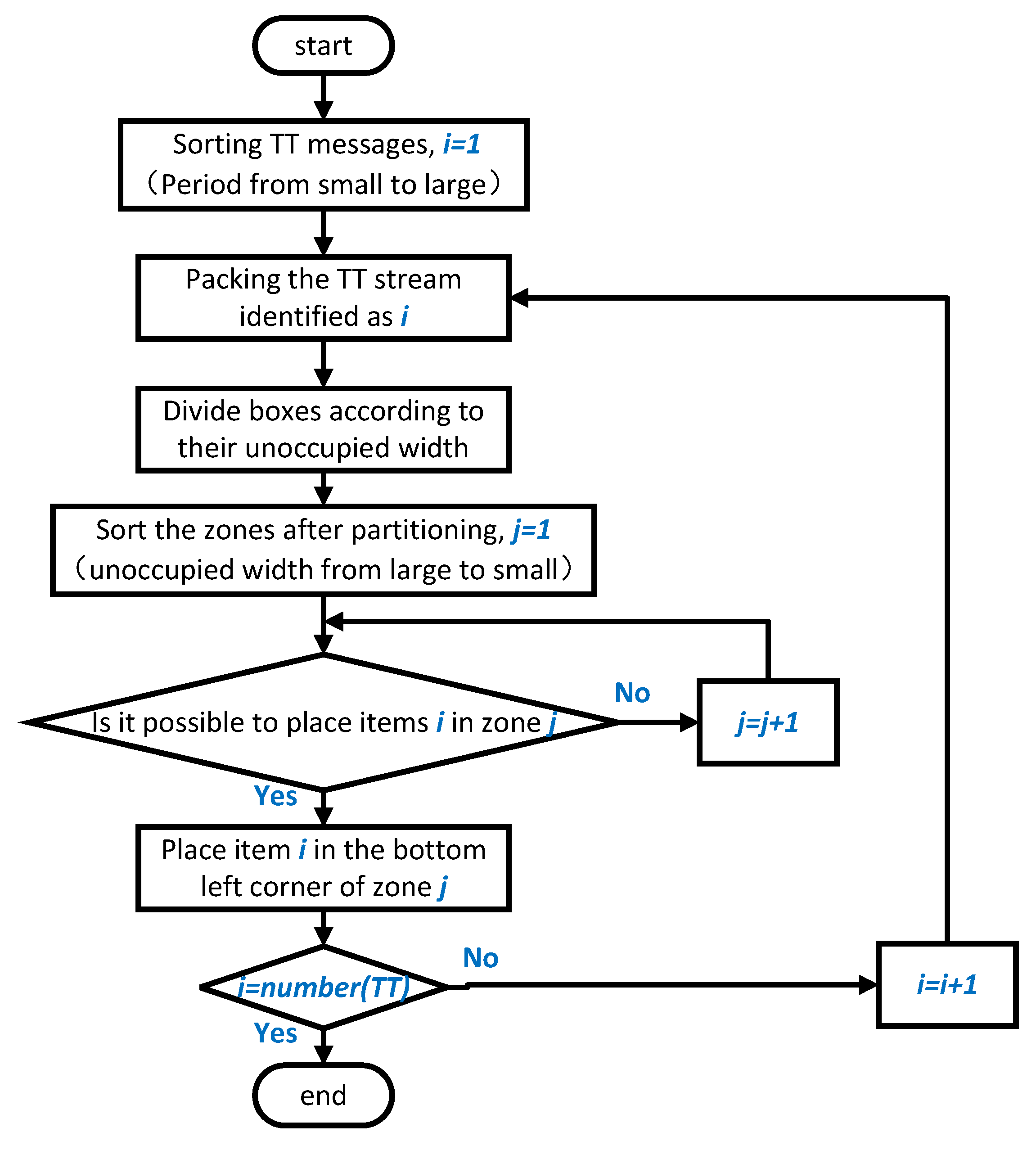
The flowchart of the CPTSA-US algorithm is shown in Figure 8.
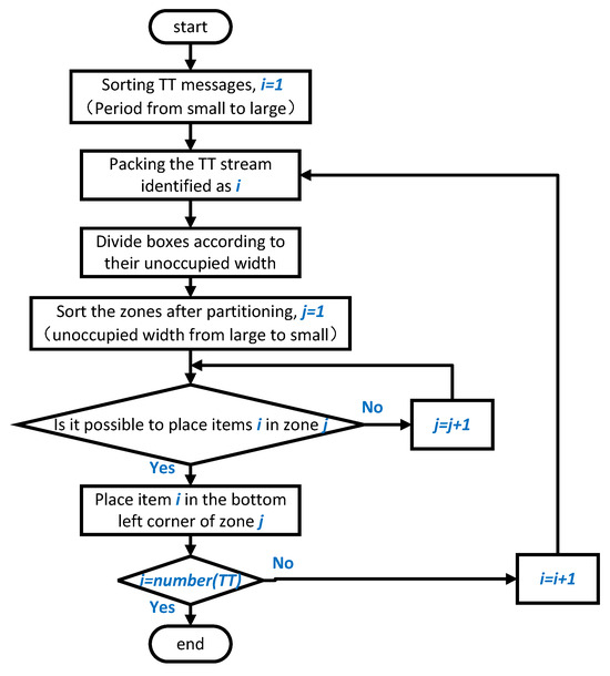
Figure 8.
The flowchart of the CPTSA-US algorithm.
Here is the computational complexity analysis of the CPTSA-US. First, sorting the items has a time complexity of , where n is the number of items. Next, initializing the space vector has a time complexity of , where His the height of the boxes. Then, the outer loop iterates through all the items n times, and the inner loop iterates through each row of the boxes H times. After that, the partition based on the remaining space in each row of the boxes, which is related to the box height, has a time complexity of . Then, sorting based on the unused space size is performed, assuming there are at most P partitions, with a time complexity of for each partition. Finally, iterating through all the partitions to place the items is completed with a worst-case time complexity of . In summary, the overall time complexity is approximately . In the worst case, if we assume that the number of partitions P is proportional to the box height H, the time complexity can be further simplified to .
4.3. Mixed-Critical Traffic Scheduling Algorithm Based on Free Time Domain (MCTSA-FTD)
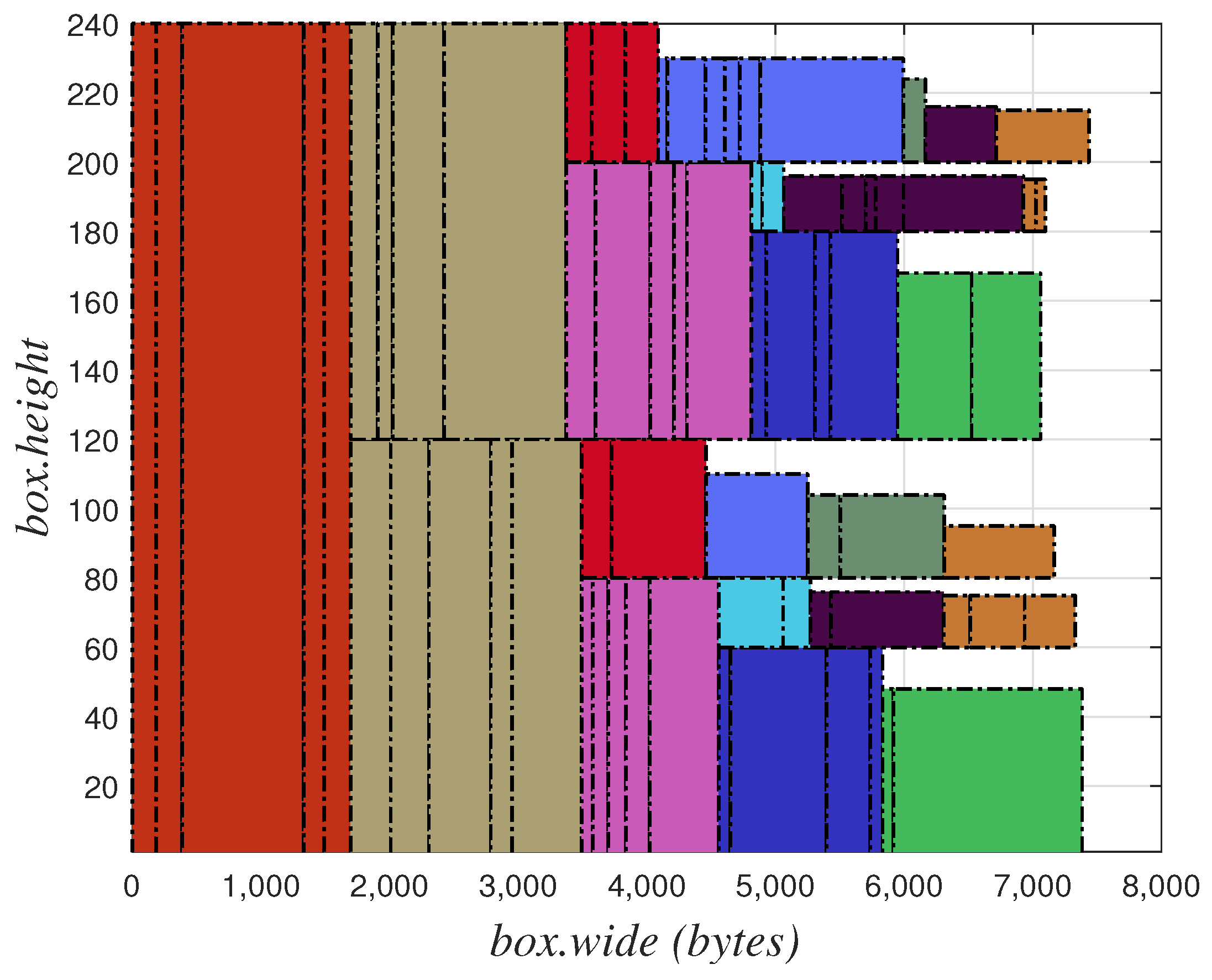
The packing results using the CPTSA-US are shown in Figure 9. Different colors in the diagram represent TT flows with different periods. It can be seen that the TT flows are compressed and transmitted in the first half of a basic period. However, if the scale of the flow increases and a large number of TT flows accumulate, the message segments for TT flows may become too long. This not only leads to the accumulation of TT flows but also increases the delay, jitter, and packet loss rate of BE flows, which subsequently increases the instantaneous burden on the network, thereby reducing the stability of the network and increasing the probability of network paralysis.
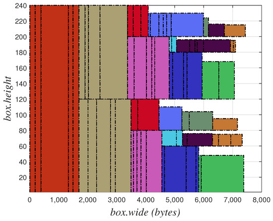
Figure 9.
Illustrative diagram of CPTSA-US packing results.
To address this issue, it is necessary to ensure the feasibility of the scheduling table while dispersing the distribution of TT flows as much as possible, providing available free time slots with relatively uniform distribution for BE flows and ensuring the transmission performance of BE flows. Therefore, this paper optimizes the CPTSA-US and proposes a mixed-critical traffic scheduling algorithm based on free time domain (MCTSA-FTD) based on it, which can provide a solution for BE flows with better transmission performance.
The MCTSA-FTD is mainly designed to ensure the dispersion of the scheduling results. Firstly, the packing space obtained by converting the time-domain resources needs to be divided into a limited number of spaces with the same height as the previous packing space and a width equal to the maximum frame length of TT flows. AS shown in Equations (14) and (15):
The maximum number of available packing spaces that can be split from packing space is
Then, based on the height and width of the available packing space and the maximum number, a packing algorithm is used to pack the items to be packed, aiming to use as few boxes as possible. Finally, the actual number of available packing spaces used for packing is obtained, which is denoted as . Based on the actual number of available packing spaces used, a one-dimensional repacking of the packing space is performed to evenly distribute the available packing space among them. This ensures the dispersed scheduling of TT flows and ensures that within each basic period there is a uniform dispersion with a quantity of and a width of at least for transmitting BE flows in the available free time slots.
The algorithm process of the MCTSA-FTD is shown in Algorithm 2.
| Algorithm 2 Mixed-Critical Traffic Scheduling Algorithm Based on Free Time Domain (MCTSA-FTD) |
|
Similarly, the MCTSA-FTD is based on the CPTSA-US and performs partitioning of the temporal resources for TSN traffic scheduling along with a two-stage bin packing. Assuming the number of partitions is S, the overall time complexity of the MCTSA-FTD algorithm can be approximated as , which simplifies to . If we assume that the number of partitions S and the height of the boxes H are proportional to the number of items n, the final time complexity can be further simplified to .
4.4. Schedule Table Calculation and Generation
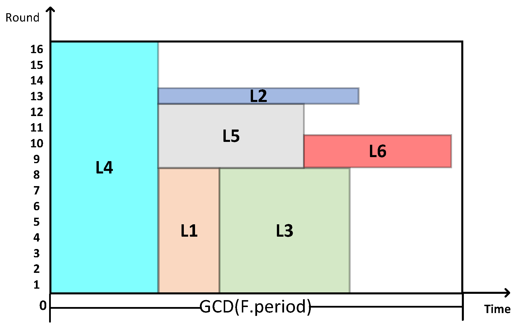
After obtaining the results through the above-mentioned traffic scheduling algorithm, it is necessary to convert the results into a traffic scheduling table. This process is obtained through the inverse transformation of the problem conversion method. As shown in Figure 10, it is a schematic diagram of the packing result, and it needs to be inversely transformed to generate the scheduling timetable.

Figure 10.
Example diagram of packing result.
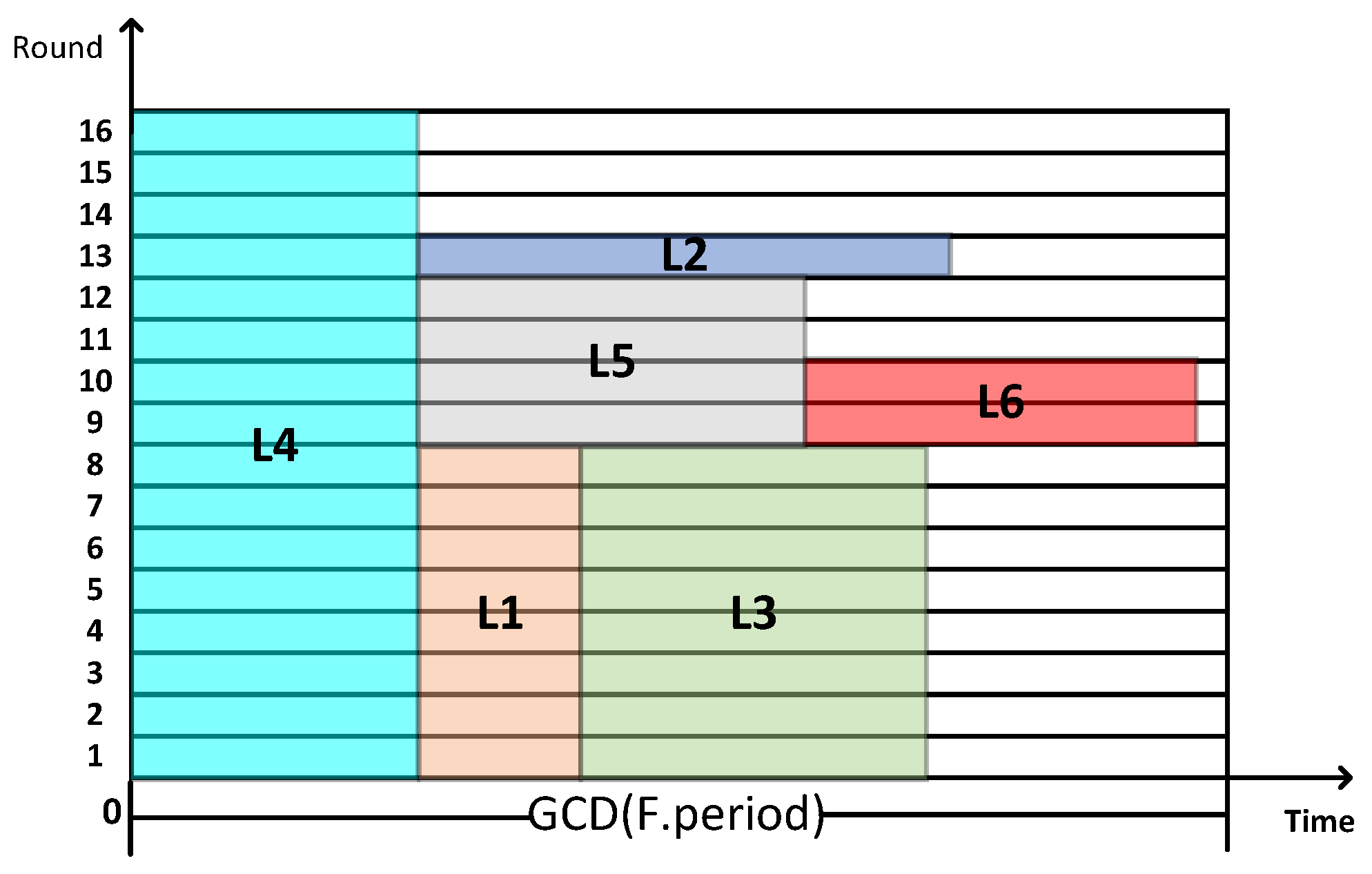
First, all two-dimensional items to be packed are divided into separate messages according to the period, and the inverse transformation of TT is completed. The result is shown in Figure 11.
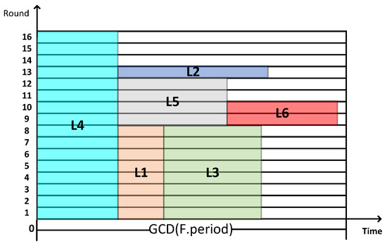
Figure 11.
Result of the two-dimensional inverse transformation of TT messages.
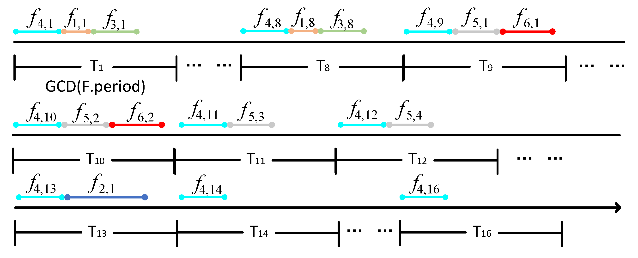
Then, according to the inverse transformation of the time-domain space, the time domain is concatenated into one-dimensional time-domain variables in the order of periods with multiple concatenated. The result is shown in Figure 12.
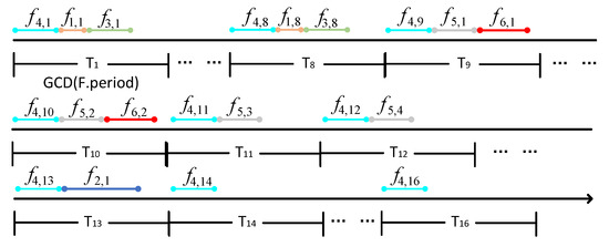
Figure 12.
Example of TT Flow Scheduling Diagram.
In the Figure 12, represents the kth transmission of TT flow within one super-period. Based on Figure 11, we can intuitively obtain the traffic scheduling timetable for the example result. It is worth noting that the scheduling timetable generated by the inverse transformation from the packing result may not strictly follow the periods of certain TT flows within one super-period. However, within each super-period, the number of transmissions for TT flows is determined by their periods, and traffic transmission is completed on a super-period basis.
Therefore, in practical scheduling, although some TT flows are not strictly transmitted according to their periods, from the perspective of one super-period, their average period of transmission equals their period parameter.
By leveraging the inverse transformation of the packing results presented in this paper, a TSN traffic scheduling table is generated. Although this approach does not transmit TT traffic strictly according to the TT flow periodic intervals, it ensures the data completeness of TT traffic within a macro-time slot. By fixing the transmission interval between TT data frames with the same identifier to a fundamental period, the overall scheduling of TT data frames with the same identifier is optimized, and the inverse transformation process is simplified. This reduces scheduling complexity, balances traffic load, and enhances the flexibility and performance of network scheduling. This method effectively addresses traffic load demands and dynamic variations while ensuring network service quality.
5. Analysis of Simulation Results
5.1. Experiment Setup
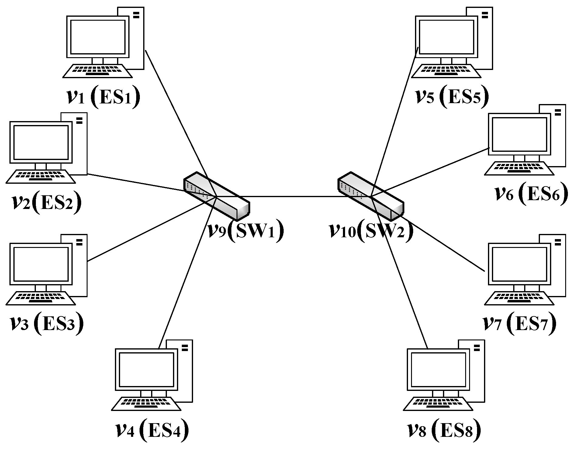
As shown in Figure 13, this paper uses a single-channel multi-line star network topology for simulation. The topology includes two switches, which are each connected to four end systems. Since the scheduling table generated by the current packing algorithm is only for unidirectional transmission, we mainly use the packing algorithm to generate the transmission scheduling table from SW1 to switch SW2. Through simulating the previous rate model, we conducted experimental tests on the two proposed algorithms. To simplify the simulation experiment, this paper assumes that the bandwidth in the network is all 1 Gbit/s. The experiment characterized various probability distributions of BE flows to simulate different TSN network application scenarios. By analyzing the delay, jitter, and packet loss rate models under different probability distributions, we verify the superiority of the MCTSA-FTD over the CPTSA-US.

Figure 13.
Network topology diagram.
5.2. Experiment Result
First, a comparison of the packing results was performed by incrementing the traffic scale by tens and generating packing results for TT flows at different traffic scales. Figure 14 shows the packing result graphs using the CPTSA-US and the MCTSA-FTD when the network traffic scales are 20, 60, and 100.
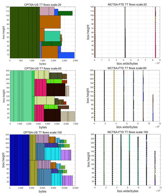
Figure 14.
Scheduling diagram for packing results of different quantities of TT flows.
By comparing the packing results of the CPTSA-US and the MCTSA-FTD, it can be observed that the MCTSA-FTD achieves a more uniform and dispersed distribution of TT flows compared to the CPTSA-US. This significantly improves the accumulation problem when applying the packing algorithm to traffic scheduling and helps reduce congestion in network traffic transmission.
5.3. Delay and Stability Analysis
In TSN, various flows are utilized to analyze network performance in terms of delay, jitter, and packet loss. In TSN, TT messages are pre-scheduled and transmitted using preemptive transmission with the highest priority only within specified time intervals. At the same time, in the context of this paper, the algorithm focuses on individual nodes, so only the transmission delay of TT flows is considered. Additionally, network failures are not taken into account, and TSN networks have achieved time synchronization. Based on the network topology, it can be determined that for TT flows in TSN, the transmission delays are as shown in Equations (17) and (18):
where is the bandwidth of data transmission, so the theoretical value of the average end-to-end delay of the entire network TT flows is as shown in Equation (19):
where represents the number of TT data frames across the entire network.
After generating the packing results of TT flows using the algorithm proposed in this paper, different probability distribution BE flows are introduced into the simulation system. The end-to-end delay of BE flows consists of two parts. As shown in Equation (20):
where represents the transmission delay of BE data, and represents the queuing delay of BE data.
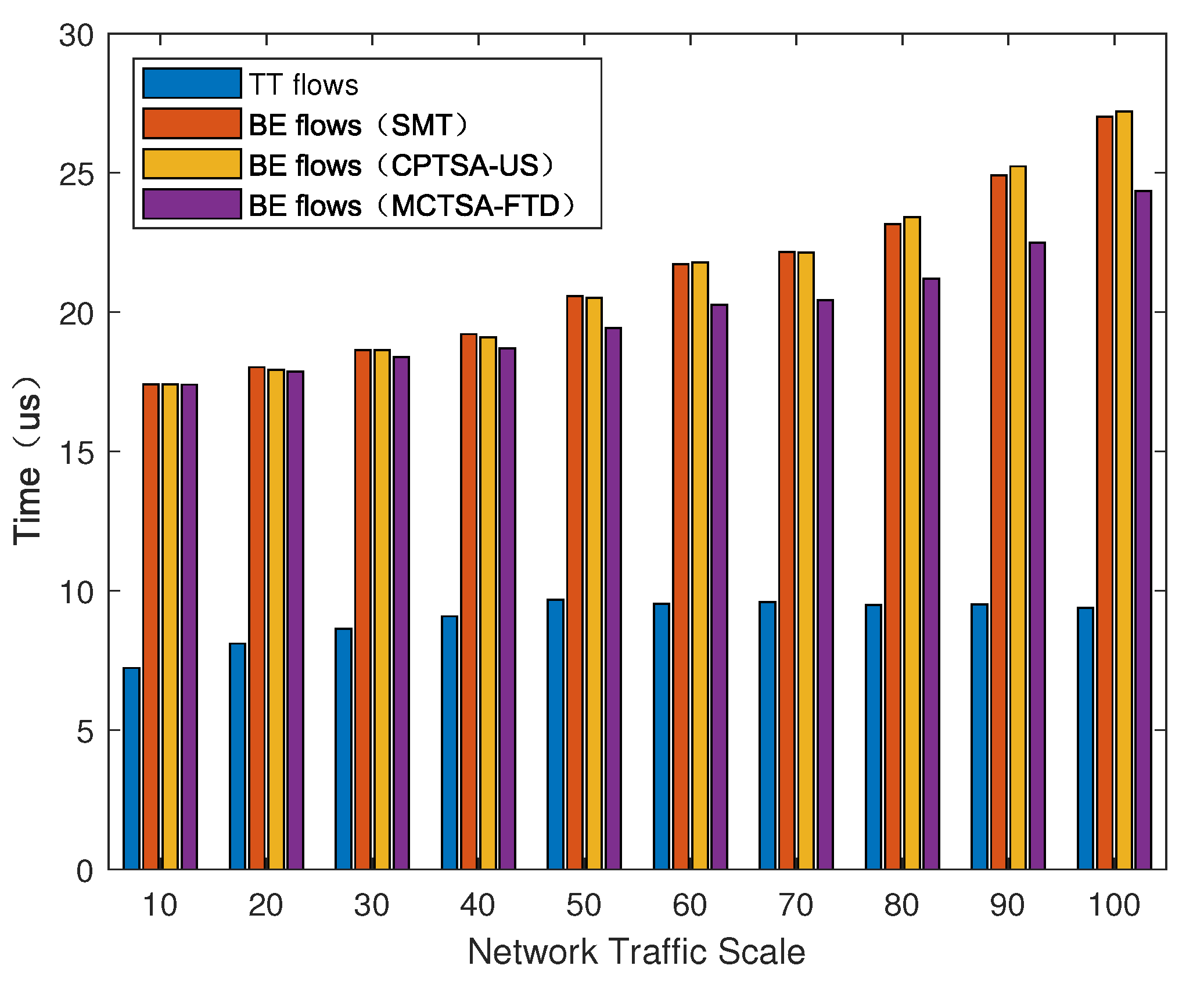
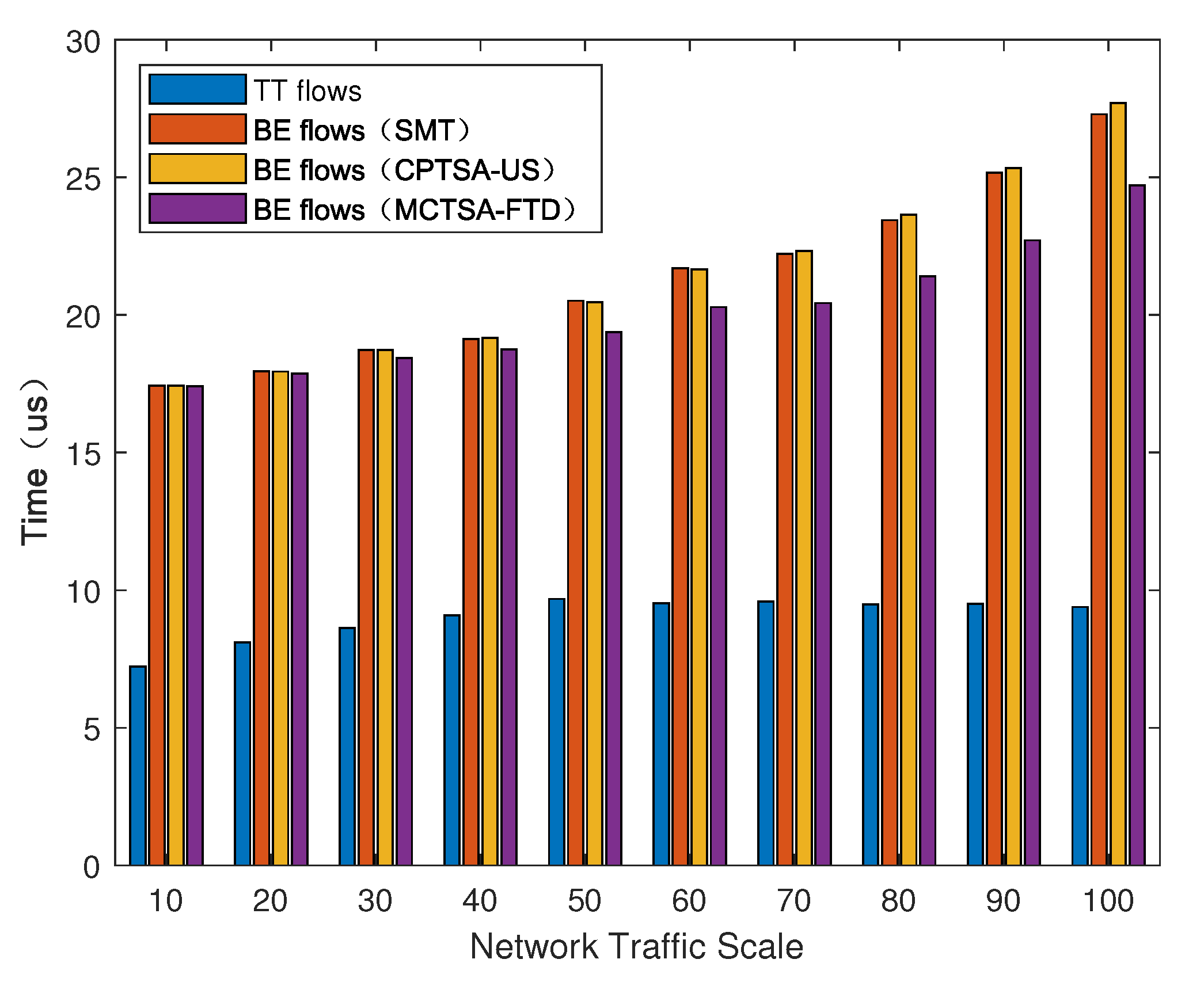
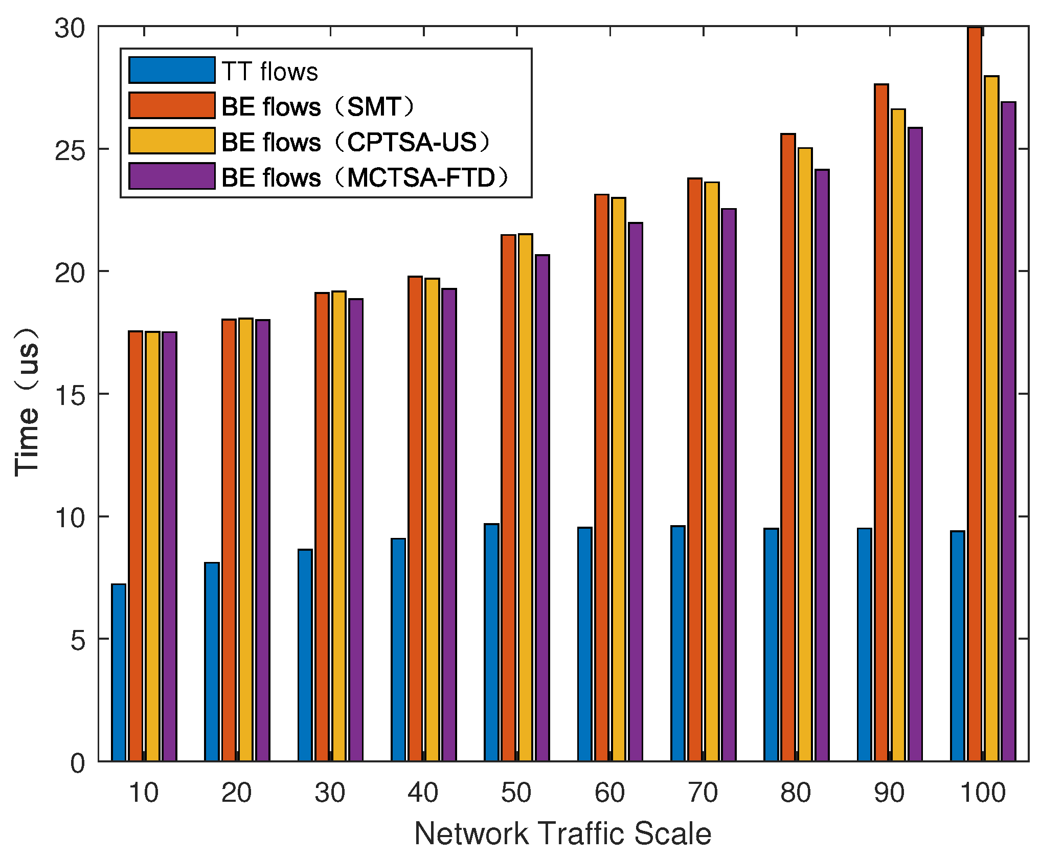
We introduced BE flows with different probability distributions to simulate different TSN application scenarios. After using the simulation model, the average end-to-end delay of various mixed-critical traffic in the entire network under different network loads is shown in Figure 15, Figure 16 and Figure 17.

Figure 15.
The average end-to-end delay of different traffic under uniform distribution for the BE flow with different algorithms.

Figure 16.
The average end-to-end delay of different traffic under normal distribution for the BE flow with different algorithms.
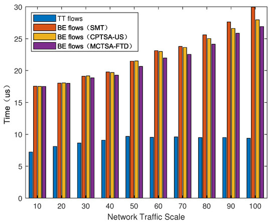
Figure 17.
The average end-to-end delay of different traffic under exponential distribution for the BE flow with different algorithms.
As shown in Figure 15, Figure 16 and Figure 17, regardless of the probability distribution of BE flows, the average end-to-end delay of TT flows is smaller and remains relatively constant with changes in network traffic volume. This is because TT flows are pre-planned with transmission time slots, using the highest priority and preemptive transmission. The average end-to-end delay of TT flows is related to its frame length and the number of switches it passes through. On the other hand, for BE flows, the average end-to-end delay is highest under an exponential distribution, which is followed by normal and uniform distributions. Furthermore, as the network traffic volume increases, the average end-to-end delay of BE flows also increases. This is because BE flow follows a first-come first-serve (FCFS) transmission mechanism, and as the number of packets in the network increases, the queuing delay significantly increases.
Next, we compared the average delay of BE flows among the traditional TSN traffic scheduling solution algorithms: SMT, CPTSA-US, and MCTSA-FTD. According to Figure 15 and Figure 16, under uniform and normal distributions, the scheduling tables generated by the SMT and the CPTSA-US exhibit similar average delays for BE flows. In Figure 17, under an exponential distribution, the CPTSA-US shows a slight improvement in average delay for BE flows compared to the SMT. This is because the initial packing algorithm accumulates TT traffic in the first half of each basic period, whereas the TSN traffic scheduling table obtained by the SMT algorithm accumulates a large amount of TT traffic at the front end of each super-period. Furthermore, regardless of the probability distribution of BE flows, the MCTSA-FTD consistently improves the end-to-end average delay of BE flows compared to the SMT and the CPTSA-US. Moreover, as network traffic increases, this difference becomes more significant, which is crucial for enhancing the transmission performance of BE flows in the network.
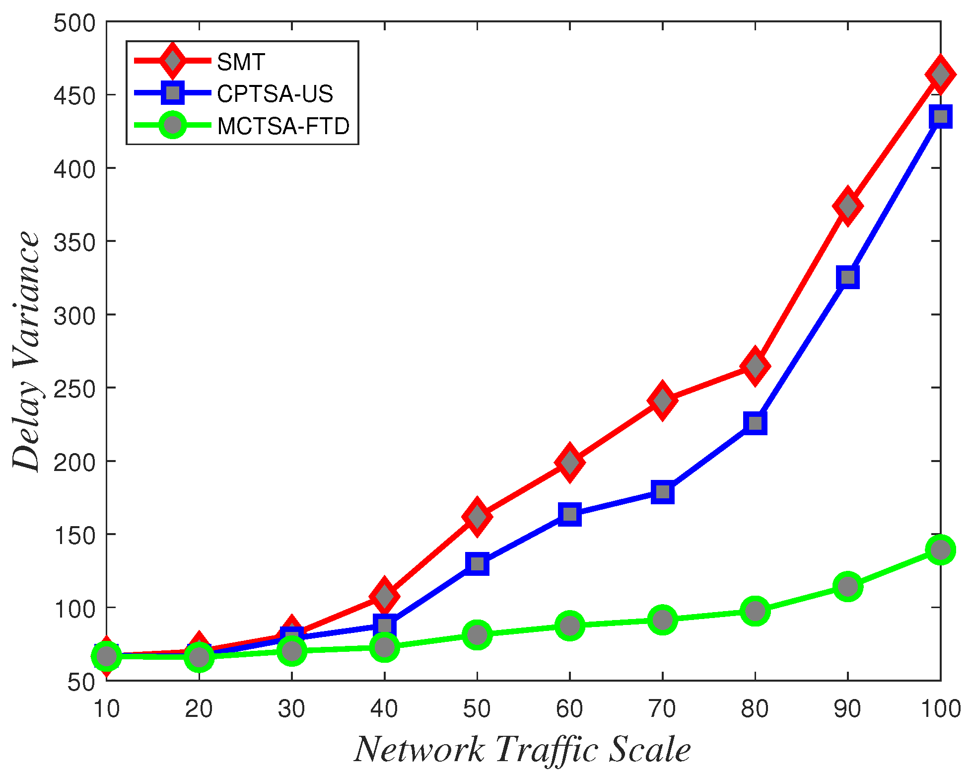
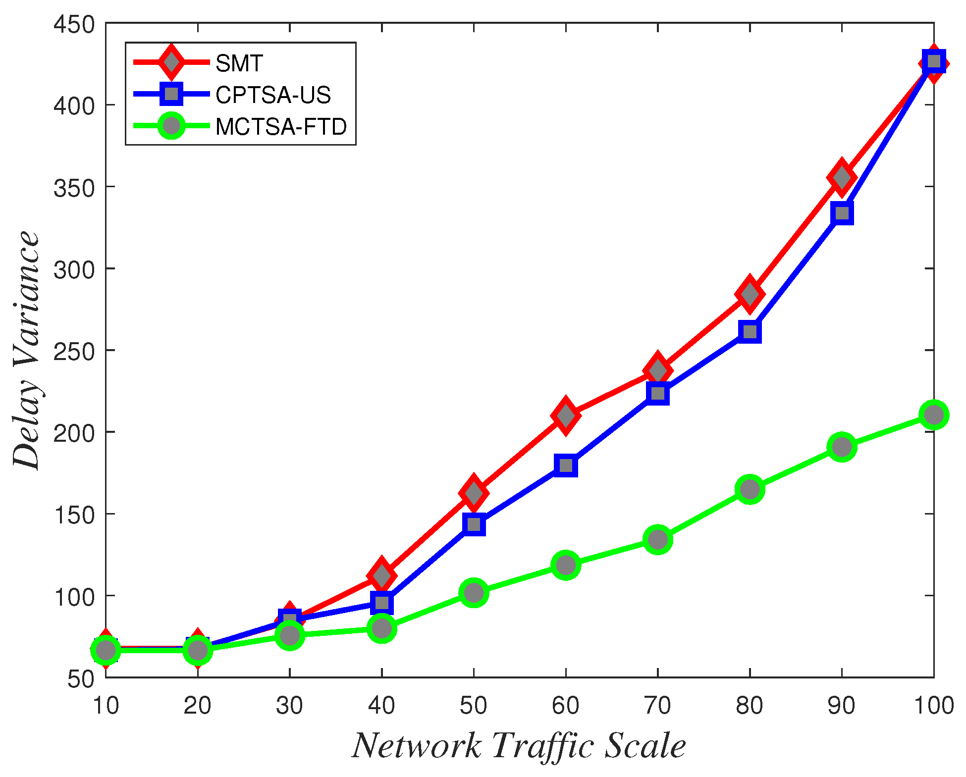
To assess the uncertainty and variability of packet transmission delays and understand how delays vary under different network conditions, delay variance analysis is crucial. According to the data depicted in Figure 18, Figure 19 and Figure 20 showing how delay variance changes with varying network traffic scales, it is evident that increasing network load leads to an increase in delay variance. Simulation results indicate that the SMT and CPTSA-US exhibit similar levels of delay variance, with the CPTSA-US slightly outperforming the SMT. Meanwhile, although the MCTSA-FTD shows an increase in delay variance with expanding network traffic, the rate of increase is notably lower compared to the SMT and the CPTSA-US. This indicates that both the CPTSA-US and the MCTSA-FTD effectively reduce delay variance in BE flows within the network, with the MCTSA-FTD showing more significant improvements. This is critical for data transmission and processing because lower delay variance ensures the stability and consistency of packet transmission, thereby reducing potential transmission errors or the need for retransmissions caused by latency fluctuations.
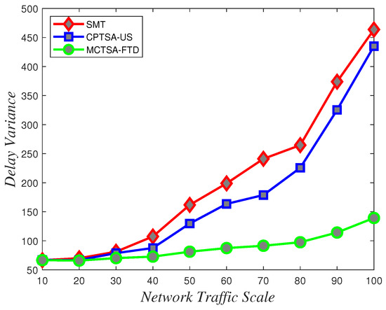
Figure 18.
Variations in delay variance for uniformly distributed BE flow under different algorithms with changing network traffic scale.
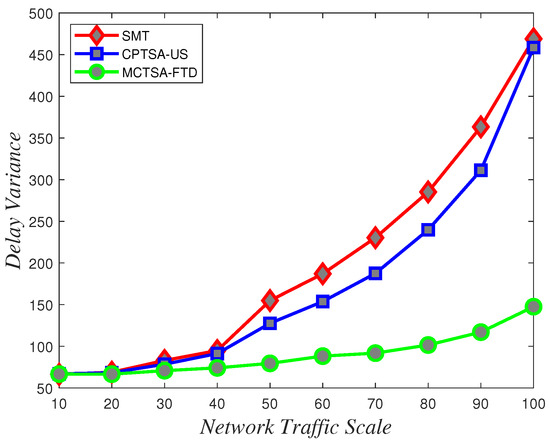
Figure 19.
Variations in delay variance for normally distributed BE flow under different algorithms with changing network traffic scale.
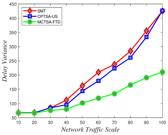
Figure 20.
Variations in delay variance for exponentially distributed BE flow under different algorithms with changing network traffic scale.
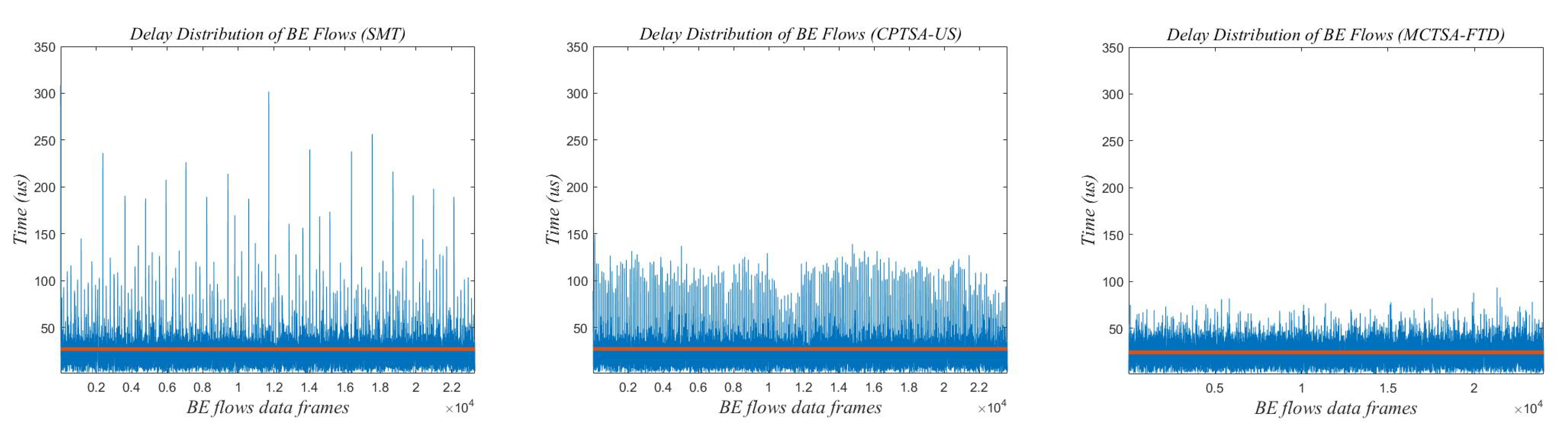
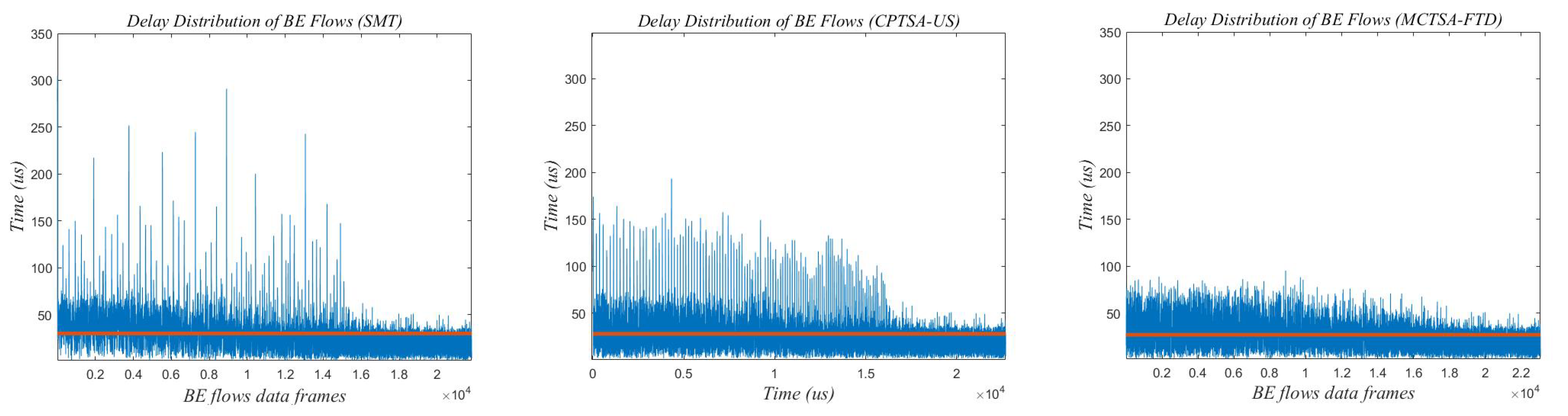
Due to the network traffic scale of 100 revealing the most significant differences in delay variance and average delay between the MCTSA-FTD, SMT, and CPTSA-US, it highlights their distinctions most prominently. Therefore, selecting this network load of 100 for a detailed analysis of delay characteristics in BE flows is warranted. Figure 21, Figure 22 and Figure 23 show the end-to-end delay of BE flows under different probability distributions when the network load is 100.
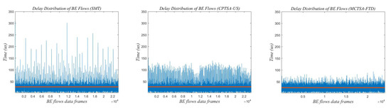
Figure 21.
The delay distribution graph of BE flow under uniform distribution when the network traffic scale is 100.
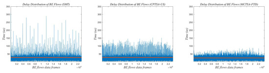
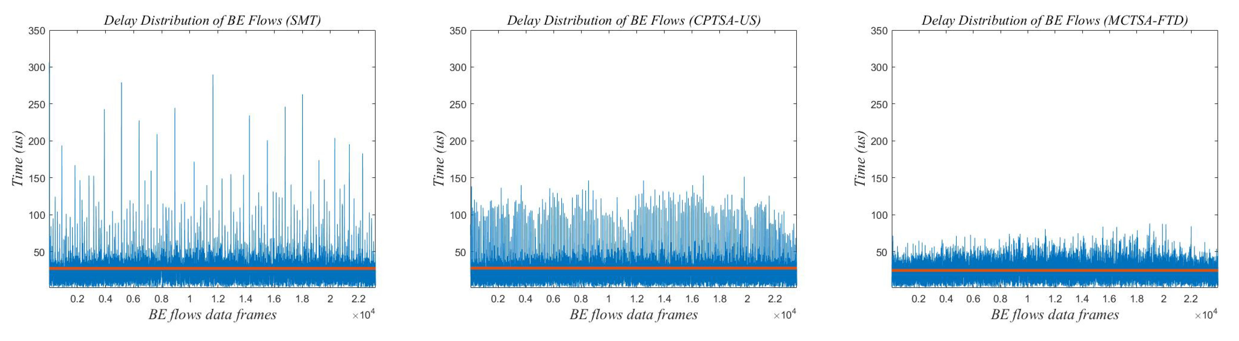
Figure 22.
The delay distribution graph of BE flow under normal distribution when the network traffic scale is 100.

Figure 23.
The delay distribution graph of BE flow under exponential distribution when the network traffic scale is 100.
The red line in Figure 21, Figure 22 and Figure 23 represents the average delay of the BE flows. From Figure 21, Figure 22 and Figure 23, it can be observed that regardless of the probability distribution of best-effort (BE) flows, when transmitting traffic according to the traffic scheduling table generated by the SMT, the maximum delay of BE flows ranges between 300 and 350 us. For the CPTSA-US, the maximum delay of BE flows is within 200 us, and for the MCTSA-FTD, the maximum delay does not exceed 100 us. This indicates that compared to SMT, both the MCTSA-FTD and CPTSA-US reduce the maximum delay of BE flows. Moreover, the MCTSA-FTD significantly reduces the maximum end-to-end delay of BE flows while also lowering the overall average delay of BE flows. Furthermore, compared to the CPTSA-US and SMT, the MCTSA-FTD exhibits a delay distribution that is more concentrated around the average delay, resulting in smaller differences between maximum and minimum end-to-end delays. These findings suggest that the scheduling table generated by the MCTSA-FTD reduces the overall waiting time for BE flows during transmission, thereby decreasing the likelihood of data loss due to excessive waiting times or the need for retransmission. This enhancement ensures a higher quality of service and improves data transmission efficiency, playing a crucial role in reducing network congestion and maintaining network stability.
5.4. Packet Loss Rate Analysis
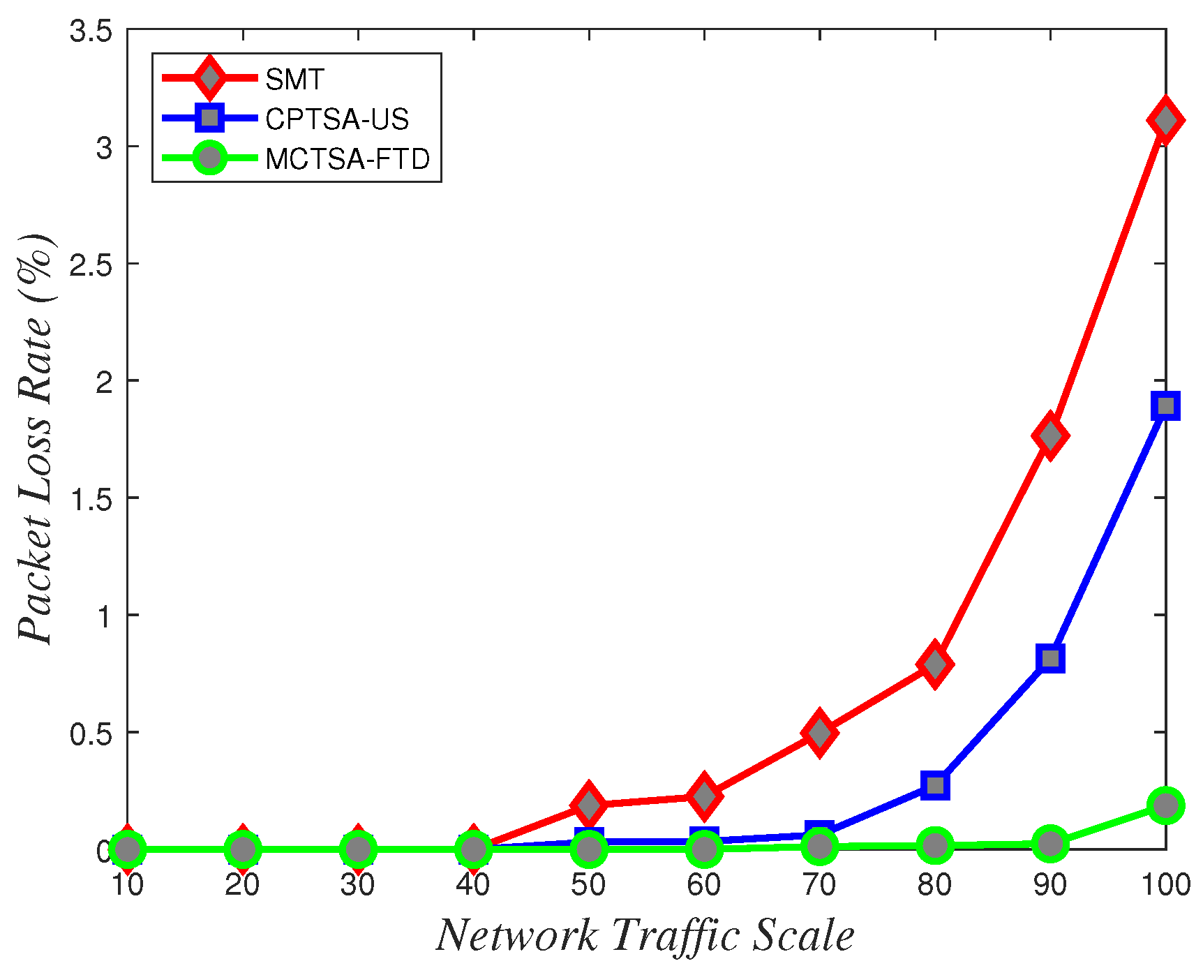
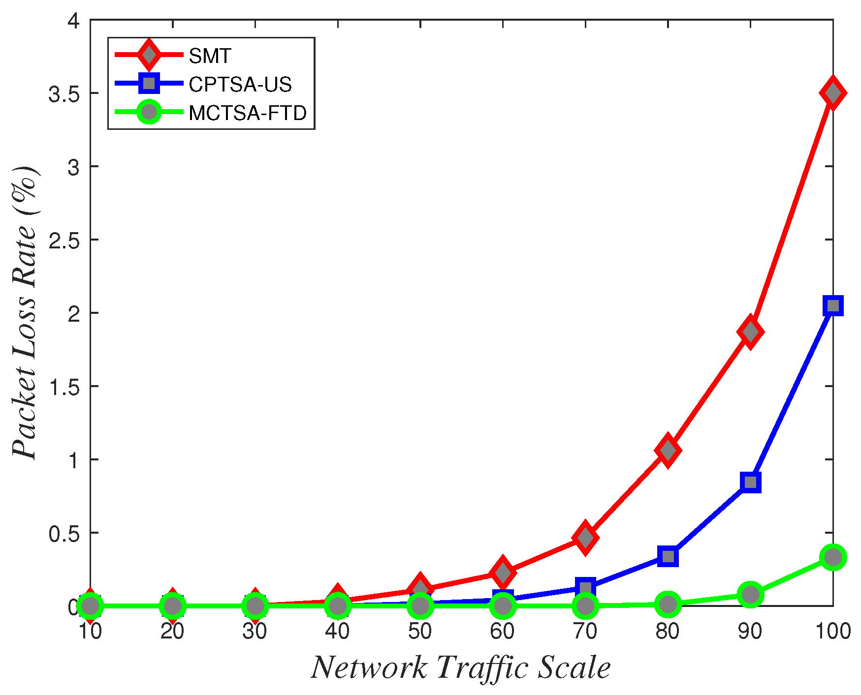
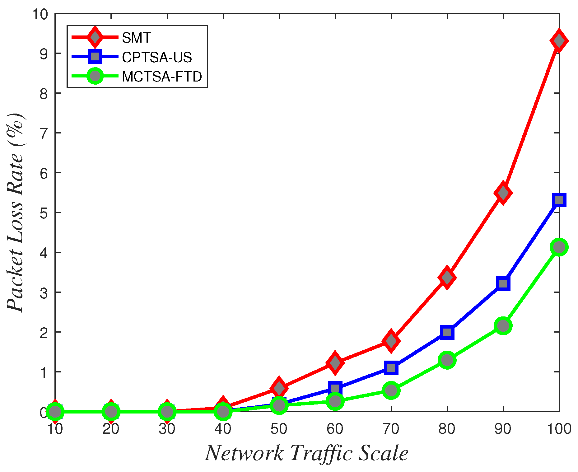
In this experiment, when the network load is low, the packet loss rates for TT and BE flows are both zero. However, as the network load increases, due to the limited communication available time resources in TSN networks and the preemptive transmission with the highest priority adopted by TT flows, its performance will not be greatly affected. The end-to-end delay of BE flows will continue to increase, resulting in packet loss due to excessive delay or limited queue number. Figure 24, Figure 25 and Figure 26 show the variation in packet loss rates with network scale under different probability distributions for the two algorithms.

Figure 24.
Packet loss rate variations with network traffic scale under different algorithms for uniformly distributed BE flow.
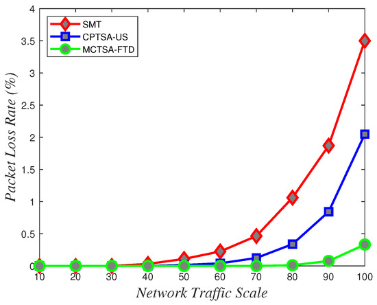
Figure 25.
Packet loss rate variations with network traffic scale under different algorithms for normally distributed BE flow.

Figure 26.
Packet loss rate variations with network traffic scale under different algorithms for exponentially distributed BE flow.
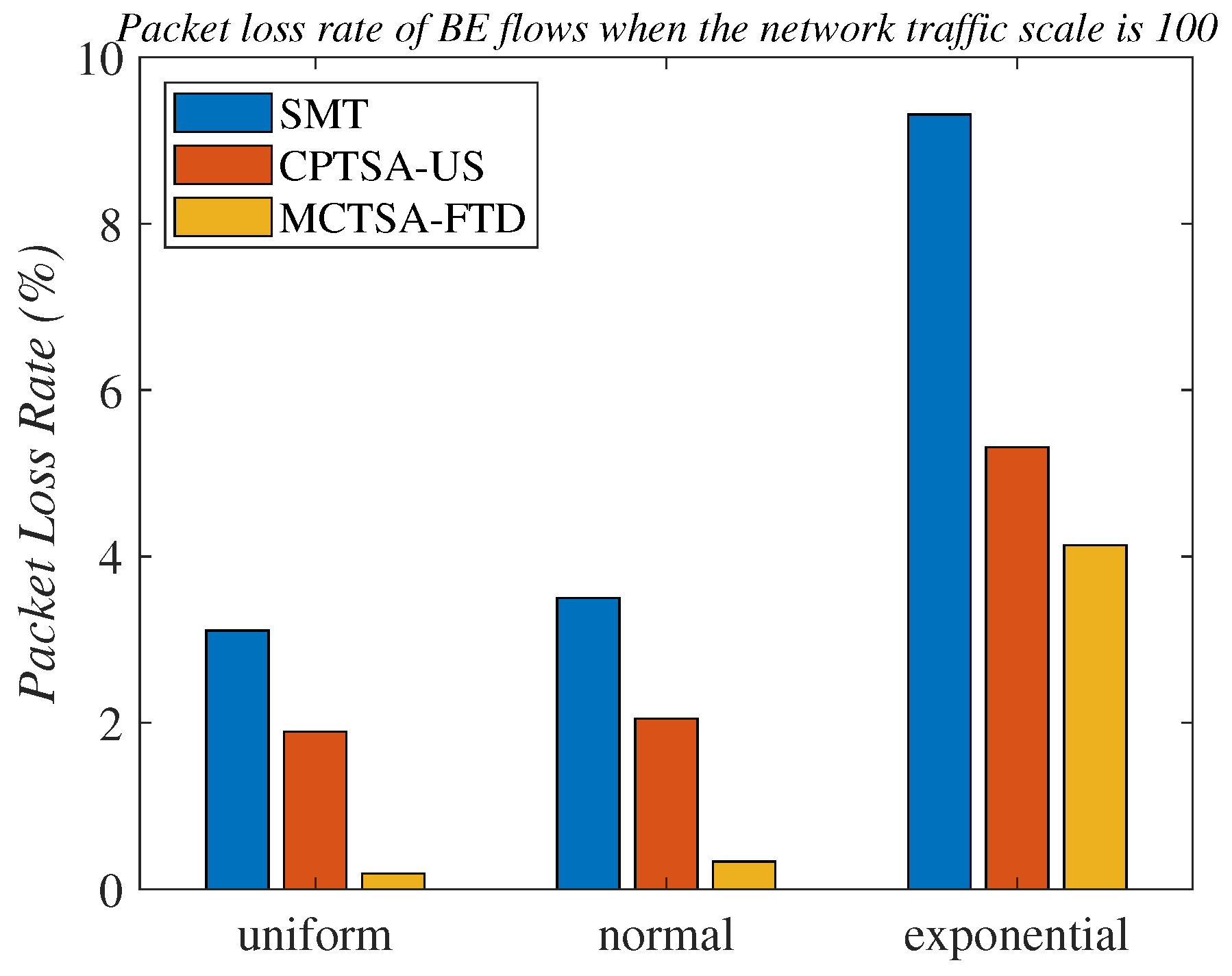
From Figure 24, Figure 25 and Figure 26, it can be observed that in line with theoretical analysis, regardless of the probability distribution of the BE flows, when the network traffic is at a small scale, the packet loss rate for BE flows is almost zero. As the network traffic scale increases, the packet loss rate for all probability distributions exponentially increases. However, under normal and uniform distributions, the MCTSA-FTD exhibits significant improvements in packet loss rates for best-effort (BE) flows compared to the CPTSA-US and the SMT, and the CPTSA-US outperforms the SMT in this regard. In scenarios involving an exponential distribution, although packet loss rates for the SMT, the CPTSA-US, and the MCTSA-FTD all exhibit exponential growth with increasing network scale, the proposed algorithms show improvements in BE flow packet loss rates compared to the SMT. Particularly, the partitioning-optimized MCTSA-FTD demonstrates notably superior performance in reducing BE flow packet loss rates.
Figure 27 and Table 1 provide detailed records of the packet loss rates of BE flows for the three algorithms under different probability distributions when the network traffic scale is 100.

Figure 27.
Packet loss rates of BE flows under different probability distributions when the network scale is 100.

Table 1.
The packet loss rate of BE flows when the network scale is 100.
Through the analysis of the above simulation results, it can be seen that we simulated BE flows under different probability distributions to simulate different TSN application scenarios. The normal distribution and uniform distribution were used to simulate scenarios with smoother traffic in the network. The exponential distribution was more suitable for simulating network application scenarios where traffic surges at certain times. Finally, comparing with the SMT, the CPTSA-US reduces the complexity of TSN traffic scheduling while also moderately decreasing the average latency of BE traffic in TSN under exponential distribution. We further observed that irrespective of the probability distribution of network traffic, the CPTSA-US enhances the stability of BE traffic transmission to some extent compared to the SMT. Subsequently, the MCTSA-FTD, proposed thereafter while maintaining TT transmission performance, effectively reduces the end-to-end average latency, jitter, and packet loss rate of BE flows, thereby further extending the advantages of the CPTSA-US.
6. Conclusions
TSN guarantees the transmission performance of various priority flows in the network with deterministic latency by specifying the transmission order and time slots of frames, meeting the deterministic low-latency network transmission requirements. However, the traffic scheduling problem in TSN is NP-hard. In this paper, to reduce the computational complexity of TSN traffic scheduling, we transformed the complex problem of TSN traffic scheduling into a non-overlapping bin packing problem and proposed the CPTSA-US algorithm to solve the TSN traffic scheduling. The feasibility of transforming the TSN traffic scheduling problem into a two-dimensional packing problem was verified through the scheduling results. Furthermore, to address the accumulation problem of TT traffic in traditional TSN traffic scheduling algorithms and the CPTSA-US, we introduced the MCTSA-FTD algorithm, which divides time resources into multiple padding spaces to achieve more efficient TT traffic dispersion scheduling. Simulation results show that the MCTSA-FTD and CPTSA-US further reduce the average latency, latency variance, maximum latency, and packet loss rate of BE traffic compared to the SMT algorithm, with the MCTSA-FTD demonstrating better performance. Specifically, when the network traffic scale is 100, the maximum latency of the SMT is around 300–350 us, while that of the CPTSA is less than 200 us, and that of the MCTSA-US does not exceed 100 us. In conclusion, the algorithms proposed in this paper bring significant optimization effects to TSN networks, including a notable reduction in the maximum latency and packet loss rate of BE traffic in the network, improving the overall transmission performance and resource utilization efficiency of the entire network. These optimizations and improvements not only significantly enhance the overall performance of the network but also lay a solid foundation for future industrial internet and time-sensitive applications, promoting the extensive application of TSN technology in high-reliability and low-latency network communications.
7. Future Work
The algorithms currently proposed only address traffic scheduling for single-node scenarios. In future work, we aim to extend these algorithms to a localized TSN network context. To achieve this, we plan to integrate packing algorithms with modern intelligent optimization techniques to orchestrate TSN traffic scheduling across the entire network. Additionally, in addressing network failure issues, it is imperative to integrate relevant protocols from IEEE 802.1Q into the design of traffic scheduling algorithms. Optimizing packing algorithms should consider more resilient and adaptive network architectures capable of automatically adjusting and optimizing resource allocation in the face of faults or attacks, ensuring network stability and performance. Building upon these foundations, the development of intelligent algorithms and systems capable of automatically identifying, locating, and repairing issues during network failures is essential to minimize service disruption and user impact.
Author Contributions
Conceptualization, L.Z., K.Z. and G.W.; methodology, L.Z. and K.Z.; software, L.Z. and K.Z.; validation, L.Z. and K.Z.; investigation, L.Z. and K.Z.; resources, H.C.; writing—original draft preparation, K.Z.; writing—review and editing, L.Z. and K.Z.; visualization, L.Z. and G.W.; supervision, G.W. and H.C.; funding acquisition, L.Z. All authors have read and agreed to the published version of the manuscript.
Funding
This work was supported in part by the National Natural Science Foundation of China under Grant 62102314 and the Natural Science Basic Research Program of Shaanxi Province under Grant 2021JQ-708 and 2022JQ-635.
Data Availability Statement
Data are contained within the article.
Conflicts of Interest
The authors declare no conflicts of interest.
References
- Li, Z.H.; Yang, S.Q.; Yu, J.H.; Deng, Y.D.; Wan, H. State-of-the-Art Survey of Deterministic Transmission Technologies in Time-Sensitive Networking. Ruan Jian Xue Bao/J. Softw. 2021, 33, 4334–4355. (In Chinese) [Google Scholar]
- Lokman, S.F.; Othman, A.T.; Abu-Bakar, M.H. Intrusion detection system for automotive Controller Area Network (CAN) bus system: A review. EURASIP J. Wirel. Commun. Netw. 2019, 2019, 184. [Google Scholar] [CrossRef]
- Zhao, L.; He, F.; Li, E.; Lu, J. Comparison of time sensitive networking (TSN) and TTEthernet. In Proceedings of the 2018 IEEE/AIAA 37th Digital Avionics Systems Conference (DASC), London, UK, 23–27 September 2018; pp. 1–7. [Google Scholar]
- Finzi, A.; Mifdaoui, A.; Frances, F.; Lochin, E. Network calculus-based timing analysis of AFDX networks with strict priority and TSN/BLS shapers. In Proceedings of the2018 IEEE 13th International Symposium on Industrial Embedded Systems (SIES), Graz, Austria, 6–8 June 2018; pp. 1–10. [Google Scholar]
- Nsaibi, S.; Leurs, L.; Schotten, H.D. Formal and simulation-based timing analysis of Industrial-Ethernet sercos III over TSN. In Proceedings of the 2017 IEEE/ACM 21st International Symposium on Distributed Simulation and Real Time Applications (DS-RT), Rome, Italy, 18–20 October 2017; pp. 1–8. [Google Scholar]
- Nguyen, V.Q.; Jeon, J.W. EtherCAT network latency analysis. In Proceedings of the 2016 International Conference on Computing, Communication and Automation (ICCCA), Greater Noida, India, 29–30 April 2016; pp. 432–436. [Google Scholar]
- Dias, A.L.; Sestito, G.S.; Turcato, A.C.; Brandão, D. Panorama, challenges and opportunities in PROFINET protocol research. In Proceedings of the 2018 13th IEEE International Conference on Industry Applications (INDUSCON), Sao Paulo, Brazil, 12–14 November 2018; pp. 186–193. [Google Scholar]
- Val, I.; Seijo, O.; Torrego, R.; Astarloa, A. IEEE 802.1 AS clock synchronization performance evaluation of an integrated wired–wireless TSN architecture. IEEE Trans. Ind. Inform. 2021, 18, 2986–2999. [Google Scholar] [CrossRef]
- Reusch, N.; Zhao, L.; Craciunas, S.S.; Pop, P. Window-based schedule synthesis for industrial IEEE 802.1 Qbv TSN networks. In Proceedings of the 2020 16th IEEE International Conference on Factory Communication Systems (WFCS), Porto, Portugal, 27–29 April 2020; pp. 1–4. [Google Scholar]
- Stüber, T.; Osswald, L.; Lindner, S.; Menth, M. A survey of scheduling algorithms for the time-aware shaper in time-sensitive networking (TSN). IEEE Access 2023, 11, 61192–61233. [Google Scholar] [CrossRef]
- Candell, R.; Montgomery, K.; Hany, M.K.; Sudhakaran, S.; Cavalcanti, D. Scheduling for Time-Critical Applications Utilizing TCP in Software-Based 802.1 Qbv Wireless TSN. In Proceedings of the 2023 IEEE 19th International Conference on Factory Communication Systems (WFCS), Pavia, Italy, 26–28 April 2023; pp. 1–8. [Google Scholar]
- Maile, L.; Voitlein, D.; Hielscher, K.S.; German, R. Ensuring reliable and predictable behavior of IEEE 802.1 CB frame replication and elimination. In Proceedings of the ICC 2022-IEEE International Conference on Communications, Seoul, Republic of Korea, 16–20 May 2022; pp. 2706–2712. [Google Scholar]
- Nasrallah, A.; Balasubramanian, V.; Thyagaturu, A.; Reisslein, M.; ElBakoury, H. Reconfiguration algorithms for high precision communications in time sensitive networks: Time-aware shaper configuration with IEEE 802.1 qcc (extended version). arXiv 2019, arXiv:1906.11596. [Google Scholar]
- Patti, G.; Bello, L.L. Performance assessment of the IEEE 802.1 Q in automotive applications. In Proceedings of the 2019 AEIT International Conference of Electrical and Electronic Technologies for Automotive (AEIT AUTOMOTIVE), Turin, Italy, 2–4 July 2019; pp. 1–6. [Google Scholar]
- Barzegaran, M.; Pop, P. Communication scheduling for control performance in TSN-based fog computing platforms. IEEE Access 2021, 9, 50782–50797. [Google Scholar] [CrossRef]
- Atallah, A.A.; Hamad, G.B.; Mohamed, O.A. Routing and scheduling of time-triggered traffic in time-sensitive networks. IEEE Trans. Ind. Inform. 2019, 16, 4525–4534. [Google Scholar] [CrossRef]
- Yan, W.; Wei, D.; Fu, B.; Li, R.; Xie, G. A Mixed-Criticality Traffic Scheduler with Mitigating Congestion for CAN-to-TSN Gateway. ACM Trans. Des. Autom. Electron. Syst. 2024. [Google Scholar] [CrossRef]
- Chahed, H.; Kassler, A. TSN Network Scheduling-Challenges and Approaches. Network 2023, 3, 585–624. [Google Scholar] [CrossRef]
- Nie, H.; Li, S.; Liu, Y. An Enhanced Routing and Scheduling Mechanism for Time-Triggered Traffic with Large Period Differences in Time-Sensitive Networking. Appl. Sci. 2022, 12, 4448. [Google Scholar] [CrossRef]
- Raagaard, M.L.; Pop, P. Optimization Algorithms for the Scheduling of IEEE 802.1 Time-Sensitive Networking (TSN); Technical Report; Technical University of Denmark: Lyngby, Denmark, 2017. [Google Scholar]
- Pahlevan, M.; Obermaisser, R. Genetic algorithm for scheduling time-triggered traffic in time-sensitive networks. In Proceedings of the 2018 IEEE 23rd International Conference on Emerging Technologies and Factory Automation (ETFA), Torino, Italy, 4–7 September 2018; Volume 1, pp. 337–344. [Google Scholar]
- Chuang, C.C.; Yu, T.H.; Lin, C.W.; Pang, A.C.; Hsieh, T.J. Online stream-aware routing for TSN-based industrial control systems. In Proceedings of the 2020 25th IEEE International Conference on Emerging Technologies and Factory Automation (ETFA), Vienna, Austria, 8–11 September 2020; Volume 1, pp. 254–261. [Google Scholar]
- Tamas-Selicean, D.; Pop, P.; Steiner, W. Design optimization of TTEthernet-based distributed real-time systems. Real-Time Syst. 2015, 51, 1–35. [Google Scholar] [CrossRef]
- Gavrilut, V.; Pop, P. Traffic-type assignment for TSN-based mixed-criticality cyber-physical systems. ACM Trans. -Cyber-Phys. Syst. 2020, 4, 1–27. [Google Scholar] [CrossRef]
- Gavrilut, V.; Pop, P. Scheduling in time sensitive networks (TSN) for mixed-criticality industrial applications. In Proceedings of the 2018 14th IEEE International Workshop on Factory Communication Systems (WFCS), Imperia, Italy, 13–15 June 2018; pp. 1–4. [Google Scholar]
- De Moura, L.; Bjorner, N. Satisfiability modulo theories: Introduction and applications. Commun. ACM 2011, 54, 69–77. [Google Scholar] [CrossRef]
- Oliver, R.S.; Craciunas, S.S.; Steiner, W. IEEE 802.1 Qbv gate control list synthesis using array theory encoding. In Proceedings of the 2018 IEEE Real-Time and Embedded Technology and Applications Symposium (RTAS), Porto, Portugal, 11–13 April 2018; pp. 13–24. [Google Scholar]
- Jin, X.; Xia, C.; Guan, N.; Xu, C.; Li, D.; Yin, Y.; Zeng, P. Real-time scheduling of massive data in time sensitive networks with a limited number of schedule entries. IEEE Access 2020, 8, 6751–6767. [Google Scholar] [CrossRef]
- Li, Q.; Li, D.; Jin, X.; Wang, Q.; Zeng, P. A simple and efficient time-sensitive networking traffic scheduling method for industrial scenarios. Electronics 2020, 9, 2131. [Google Scholar] [CrossRef]
- Zhang, M. Research on Approximation Algorithms for Online Bin Packing and Hybrid Flowshop Scheduling Problems. Ph.D. Thesis, Dalian University of Technology, Dalian, China, 2019; pp. 20–72. (In Chinese). [Google Scholar]
- Wang, H. Research on Performance Optimization and Evaluation Technology of Time Trigged Ethernet for DIMA Applications. Ph.D. Thesis, Xidian University, Xi’an, China, 2019; pp. 55–70. (In Chinese). [Google Scholar]
- Luan, B. Research on Time Triggered Service Scheduling Algorithm in Time Triggered Ethernet. Master’s Thesis, Xidian University, Xi’an, China, 2019; pp. 11–21. (In Chinese). [Google Scholar]
- Syed, A.A.; Ayaz, S.; Leinmvller, T.; Chandra, M. MIP-based joint scheduling and routing with load balancing for TSN based in-vehicle networks. In Proceedings of the 2020 IEEE Vehicular Networking Conference (VNC), New York, NY, USA, 16–18 December 2020; pp. 1–7. [Google Scholar]
- Xue, J.; Shou, G.; Liu, Y.; Hu, Y. Scheduling Time-Critical Traffic with Virtual Queues in Software-Defined Time-Sensitive Networking. IEEE Trans. Netw. Serv. Manag. 2023. [Google Scholar] [CrossRef]
- Deng, L.; Xiao, X.R.; Liu, H.; Li, R.; Xie, G. A low-delay AVB flow scheduling method occupying the guard band in Time-Sensitive Networking. J. Syst. Archit. 2022, 129, 102586. [Google Scholar] [CrossRef]
- Ojewale, M.A.; Yomsi, P.M.; Nikolic, B. Worst-case traversal time analysis of tsn with multi-level preemption. J. Syst. Archit. 2021, 116, 102079. [Google Scholar] [CrossRef]
- Zheng, X.; Liu, Y.; Zhan, S.; Xin, Y.; Wang, Y. A novel low-latency scheduling approach of TSN for multi-link rate networking. Comput. Netw. 2024, 240, 110184. [Google Scholar] [CrossRef]


Disclaimer/Publisher’s Note: The statements, opinions and data contained in all publications are solely those of the individual author(s) and contributor(s) and not of MDPI and/or the editor(s). MDPI and/or the editor(s) disclaim responsibility for any injury to people or property resulting from any ideas, methods, instructions or products referred to in the content. |
© 2024 by the authors. Licensee MDPI, Basel, Switzerland. This article is an open access article distributed under the terms and conditions of the Creative Commons Attribution (CC BY) license (https://creativecommons.org/licenses/by/4.0/).