Inertia–Active Power Filter Design Based on Repetitive Control

Abstract

The advent of distributed generation has brought with it a plethora of challenges for the nascent power systems that are being deployed on a large scale. Firstly, the majority of power electronic converters connected to the grid are in current source mode, which results in a lack of inertia and an inability to provide effective inertia or achieve damping support during fluctuations in grid frequency. Secondly, the issue of power quality, caused by the presence of harmonics, is becoming increasingly severe. This is particularly problematic in microgrids or systems with high line impedance, where harmonics can be amplified, thereby further compromising the stability of the power system. To address the deficiency in system inertia, numerous scholars are currently utilizing grid-forming (GFM) technology to achieve virtual inertia. In order to address the issue of system harmonics, it is possible to install active power filter (APF) devices at the point of common coupling (PCC), which serve to mitigate the effects of harmonics. This paper puts forth a proposal for the implementation of an APF with virtual inertia, based on PR + RC composite control. This composite control mechanism serves to enhance the harmonic suppression capabilities of the APF. The introduction of a frequency droop enables the capacitor voltage amplitude to be adjusted during fluctuations in system frequency, thereby achieving virtual inertia and providing active support for system frequency. The experimental results demonstrate that this strategy not only reduces the total harmonic distortion (THD) by 13% in comparison to PI control, indicating excellent harmonic suppression performance, but also allows the system to be inert, achieving positive results in suppressing frequency fluctuations during transients.

1. Introduction

As the transition to new energy sources continues to deepen, there has been a significant increase in the installed capacity of renewable energy generation and a high proportion of power electronic devices connected to the grid. This has led to profound changes in the production structure, operating mechanisms, and functional forms of power systems. Issues such as low inertia, low damping, and high harmonics have become prominent, increasing the risk of stability problems related to frequency and power quality, due to the imbalance between power supply and demand. Consequently, the safety and stability of modern power systems face more severe challenges [1,2,3].

To address inertia issues, scholars have proposed various solutions involving virtual inertia [4,5,6], such as VSG technology [7]. VSG technology introduces a difference between the system frequency and the reference frequency, simulating the droop characteristics and rotor motion equations of synchronous generators through a first-order inertia component, introducing virtual inertia into the system. VSG technology enables grid-connected inverters to behave like synchronous generators, providing more stable support in the face of load surges or generation side fluctuations [8]. The literature [9] introduces an optimized, intelligent fractional-order integral (iFOI) controller for virtual inertia control (VIC) applied to the load frequency control (LFC) of interconnected modern power systems across two regions. It employs an efficient metaheuristic optimization technique known as the grey wolf optimizer (GWO) to design the proposed iFOI controller, which minimizes system frequency deviations and tie-line power deviations. The performance under load/renewable energy source (RES) fluctuations is compared, confirming the effectiveness of the proposed controller in regulating the frequency of interconnected modern power systems under the application of VIC. The literature [10] proposes the use of bidirectional virtual inertia support to enhance the stability and reliability of hybrid AC/DC microgrids under weak grid conditions. This strategy employs virtual inertia as a buffer to mitigate rapid changes in DC bus voltage and AC frequency, thereby increasing the system stability margin. The results show significant improvements in the minimum grid frequency, the rate of change of frequency (RoCoF), and deviations in the DC bus voltage for hybrid AC/DC microgrids.

To address harmonic issues, scholars have proposed various solutions like RC [11], PMR [12], LADRC [13], adapt PI [14], and MPC [15], which are designed to solve harmonic problems generated by the inverters themselves. When there are nonlinear loads in the system, additional harmonic mitigation devices are required to solve the harmonic problems in the power system. Active power filters (APFs) are effective tools for addressing harmonic issues in power systems. By monitoring and compensating for harmonics in real-time, APFs can significantly enhance power quality, particularly in environments with a large number of nonlinear loads. Notably, [16] proposes stability analysis and parameter design when considering grid impedance variations. The control strategy employed by an APF is comparable to that of most grid-connected inverters, such as adopting a PI+ fuzzy control scheme [17] and proposing a PI controller structure based on fuzzy control. The harmonic suppression effects were compared, but this scheme requires the design of fuzzy control rules, which is not conducive to engineering applications and practical project design. A model predictive control (MPC) scheme is adopted, which compares the performance of APF shunt current control techniques based on the grid current’s THD and the reference current’s tracking response time. However, this scheme requires high model accuracy, involves significant computational complexity for optimization, and necessitates designing different models for different scenarios, which is not conducive to engineering applications [18]. A PMR scheme is adopted, proposing a cascaded voltage control method for a three-phase, four-leg inverter based on a proportional multi-resonant (PMR) controller. This scheme tunes the resonances to the fundamental and main harmonic frequencies to achieve the necessary harmonic compensation. However, the design involves numerous parameters, and different tuning parameters are required for different scenarios, which is not conducive to practical project design [19]. A PI scheme is adopted, proposing the use of a proportional–integral (PI) algorithm to achieve current tracking and stability control for the APF. However, this scheme has a simple algorithm with limited harmonic mitigation capabilities and can be optimized with more suitable algorithms [20]. A LADRC scheme is adopted, proposing an improved single-phase inverter voltage control strategy, based on a composite SRFPI and LADRC. This strategy achieves low total harmonic distortion (THD), minimal steady-state and voltage tracking errors, and a rapid transient response. However, the scheme involves numerous design parameters, and the harmonic suppression effect is limited. The introduction of the integral component I leads to many side effects, such as making the closed-loop response sluggish and causing oscillations, making it unsuitable for engineering applications [21]. A repetitive control scheme is adopted, involving the design of a repetitive controller to mitigate disturbances caused by unbalanced filter parameters. However, this scheme has poor dynamic performance and is less effective compared to composite repetitive control [22].

To address the issues of frequency fluctuations and power quality problems in power systems caused by nonlinear loads and the large-scale integration of renewable energy, while enhancing the harmonic suppression capabilities of APFs, this paper adopts a design based on composite repetitive control and PR control strategies. This design combines the fast response of PR control with the precise tracking of repetitive control to achieve efficient harmonic suppression. Additionally, by implementing voltage droop control on the DC-side voltage external loop, the APF’s virtual inertia is increased, providing transient frequency support during grid frequency fluctuations. This design only requires improvements to the APF’s control algorithm, without the need for additional hardware design.

This paper presents a control method for active power filters that addresses frequency fluctuations and power quality issues in power systems caused by nonlinear loads and the large-scale integration of renewable energy sources. In addition to enhancing harmonic suppression capabilities, the method also adds virtual inertia into the APF, thereby providing transient frequency support during grid frequency fluctuations. This article commences with an introduction to the research background and the current state of thinking in the field, followed by a description of the design of PR and RC controllers through modelling and stability analysis. Subsequently, the parameter design for virtual inertia is undertaken in order to ensure that the resulting value remains within a reasonable range. Subsequent experimental demonstrations serve to validate the effectiveness of harmonic suppression under conditions of nonlinear load and to verify the presence of inertia during sudden changes in load. The paper concludes with a summary of the conclusions reached.

2. Proposed Control Strategy and Stability Analysis

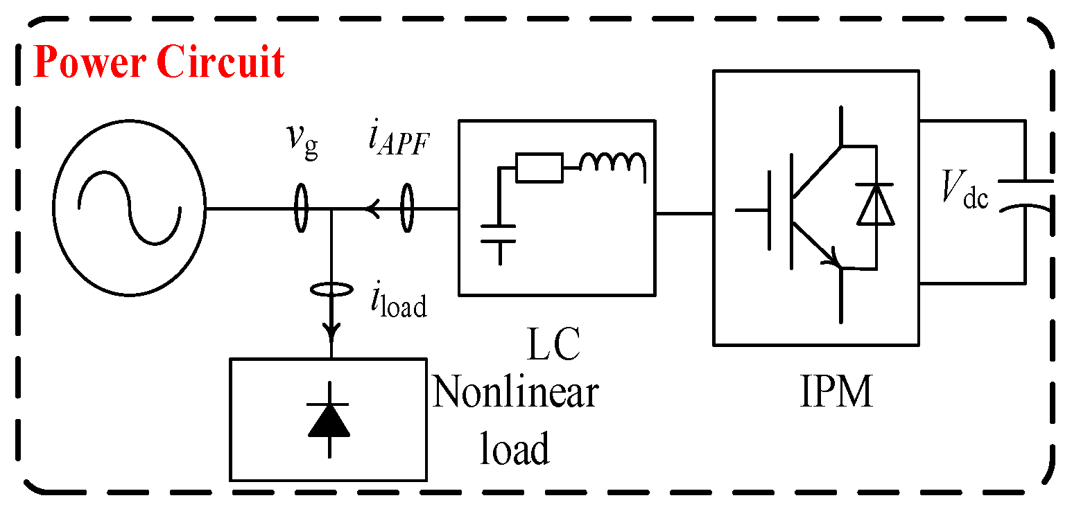
A block diagram of the active power filter (APF) with virtual inertia, based on proportional-resonant and repetitive control, is presented in Figure 1. In the inverter unit, an LC filter network is composed of an inverter bridge circuit, an inductor L_f, and a capacitor C_f. Here, i_load represents the load current, v_g is the grid voltage, and i_g is the APF output current. The frequency f_g is obtained from the v_g through a phase-locked loop and compared with the reference frequency f_ref, which, through the frequency–voltage outer loop, gives the APF inertia. Simultaneously, the fundamental component of the i_load is extracted to obtain the harmonic current i_H, and the proportional-resonant and repetitive control are used to adjust the i_APF output current, achieving tracking and compensation of the harmonic current, thus completing the harmonic mitigation.

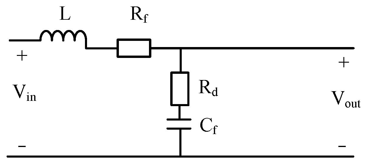
According to the inverter circuit in Figure 1, the transfer function of the controlled object P(s) for the system under no-load conditions is easily obtained as follows:

$$P\left(s\right)=\frac{s{C}_f{R}_d+1}{s^{2}L{C}_f+s{C}_f\left(R_d+R_f\right)+1}$$

(1)

The detailed derivation process can be found in Appendix A.

R_f is the equivalent resistance of the inductor and the circuit. R_d is the damping resistor. The parameters of the active power filter (APF) system are presented in

Table 1. Active power filter (APF) system parameters.

Parameter	Value
Vdc	800 V
Rf	0.1 Ω
Lf	3 mH
Rd	1 Ω
Cf	10 uF
fr	50 Hz
fc	10 kHz
Ts	1 × 10−4 s
Vg	380 V
H (inertia rating)	5 s

.

In Figure 2, the repetitive control part mainly consists of two major components: the internal model and the compensation segment. The internal model z^−N/(1 − Q(z)z^−N) integrates the error signal e(z) per cycle. When Q(z) = 1, it achieves zero steady-state error control for external signals. Moreover, z^−N provides the necessary phase lead component for the system, but this results in a one-cycle delay in the system output. The compensation segment C(z) = k_rz^kS(z) provides phase and amplitude compensation, where k_r is the gain of the repetitive controller; z^k is the lead segment to compensate for the lag in the phase and frequency response of the control object and filter; and S(z) is generally a combination of low-pass filters and notch filters, primarily ensuring that the controlled object’s mid- and low-frequency gain is 1, with rapid attenuation at high frequencies, thereby reducing the design difficulty of the repetitive controller and enhancing the system’s stability and anti-interference capability.

When the system is stable, the tracking error e(z) of the composite control is given by:

$$e(z)=\frac{[1-Q(z)z^{-N}][r(z)-d(z)]}{[1+G_{pr}(z)P(z)]\{1-z^{-N}[Q(z)-\frac{C(z)P(z)}{1+G_{pr}(z)P(z)}\left]\right\}}$$

(2)

Let $P_0(z)/[1+G_{pr}(z)P(z)]$.

$H_1\left(z\right)=1+G_{pr}\left(z\right)P\left(z\right)$, $H_2(z)=1-z^{-N}[Q(z)-C(z)P_0(z)]$. Thus, the system’s characteristic polynomial H(z) is given by:

$$H\left(z\right)=H_1\left(z\right)H_2\left(z\right)$$

(3)

For system stability, Equation (3) must satisfy the requirement that the roots of $H_1\left(z\right)$ and H₂(z) are both inside the unit circle. When the PR controller controls the inverter alone, the closed-loop system transfer function’s characteristic polynomial is H₁(z); for the control object P₀(z) under the sole action of repetitive control, the closed-loop system transfer function’s characteristic polynomial is $H_2\left(z\right)$. Hence, for this form of composite control, when the sole PR control acting on the inverter is stable, it satisfies the requirement that the roots of $H_1\left(z\right)$ are within the unit circle; to also have the roots of $H_2\left(z\right)$ within the unit circle, it is equivalent to maintaining the stability of the control object $P_0\left(z\right)$ under the sole action of repetitive control.

The closed-loop system characteristic equation when repetitive control acts alone is:

$$H_2\left(z\right)=1-z^{-N}\left[Q\left(z\right)-C\left(z\right)P_0\left(z\right)\right]=0$$

(4)

For system stability, it must satisfy the following:

$$\left|z^{-N}\left[Q\left(z\right)-C\left(z\right)P_0\left(z\right)\right]\right|<1$$

(5)

When the inverter output frequency is the fundamental frequency and there are integer multiples, it is known that z^−N = 1 can derive the conditions for stability as:

$$|Q\left(z\right)-k_r{z}^{k}S\left(z\right)P_0\left(z\right)|<1\hspace{1em}\forall z=e^{jw},0<w<\frac{\Pi }{T_s}$$

(6)

The detailed derivation process can be found in Appendix B.

3. Proposed Controller Parameter Design

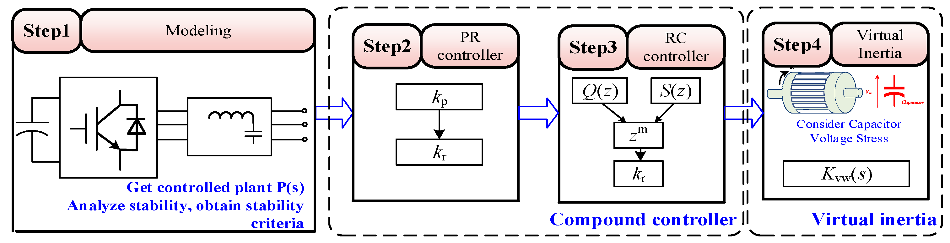
The parameter design is divided into inertia droop coefficient design and composite controller design. First, the composite controller is designed to ensure the basic functions are achieved. Then, the inertia droop can be designed as an additional software component. The design process is as follows:

According to Figure 3, first, model the system to obtain the transfer function of the controlled object. Then, use traditional control theory to design the parameters of the PR controller, starting with k_p followed by k_r. For the design of the repetitive control, the PR controller and the controlled object P(s) form a new generalized controlled object. The design of Q(z) and S(z) has no specific order. And then, design the phase compensation element to compensate for the phase delay of the generalized controlled object and increase the system’s phase margin. Finally, design the repetitive control gain element. After completing steps 2 and 3, the composite controller design is complete, and you can proceed to design the virtual inertia element. Based on the capacitor voltage stress, select the appropriate frequency–voltage droop coefficient k_vw(s). At this point, the parameter design for the control part of the proposed controller is complete.

3.1. PR Controller Design

As mentioned earlier, the stability of the PR controller must be ensured, first in the design of the composite controller. The expression for the proportional-resonant controller is given by:

$$G_{pr}\left(s\right)=K_p+\frac{K_{r}s}{s^2+w^2}$$

(7)

In this expression, $K_p$ is the proportional coefficient, K_r is the resonant controller coefficient, and w is the resonant frequency. This object only considers the zero-order hold (ZOH) discretization method; therefore, the discrete expression for $G_{pr}\left(s\right)$ under the ZOH method is:

$$G_{pr}\left(z\right)=K_p+\frac{K_r(z^{-1}-z^{-2})}{1-2\cos \left(w{T}_s\right)z^{-1}+z^{-2}}$$

(8)

In contrast to proportional controllers, resonant controllers only affect the frequency at the resonance point, having minimal impact at other frequencies. Therefore, when selecting the proportional parameter K_p, the resonant controller is initially disregarded, and then the appropriate proportional parameter is used to design the resonant controller K_r.

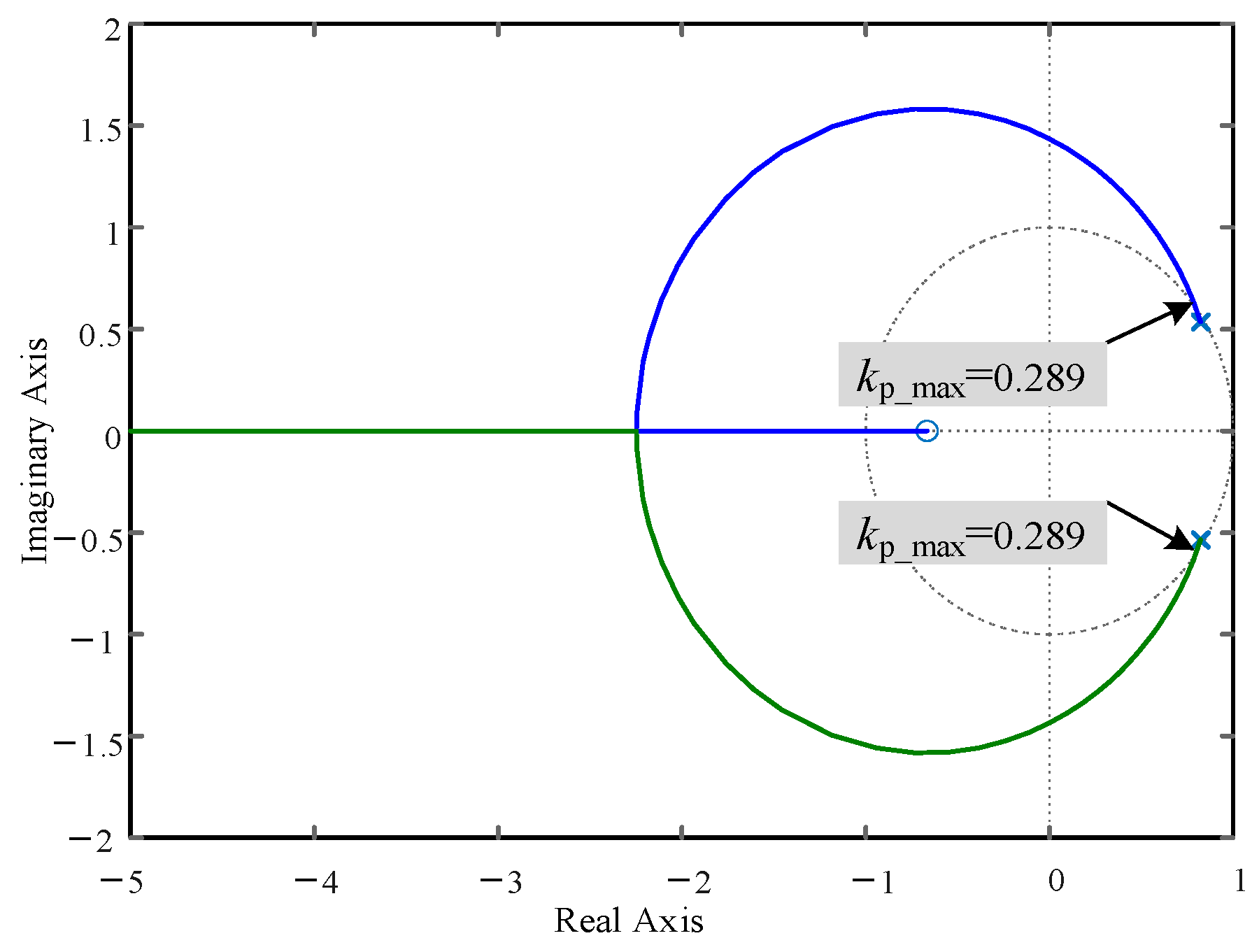
3.1.1. Proportional Coefficient K_p Design

When the controlled object is solely using proportional control, based on Equation (1) and the parameters in Table 1, the open-loop transfer function expression of the control system discretized using the “ZOH” method is:

$$G_p\left(z\right)=\frac{K_{p}0.1911z+0.1272}{z^2-1.646z+0.964}$$

(9)

From this, the root locus, as shown in Figure 4, can be drawn to determine the range of the K_p values.

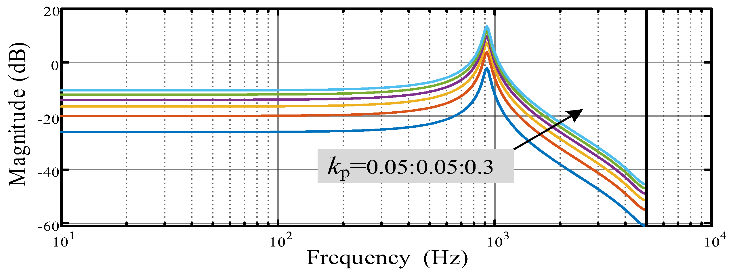
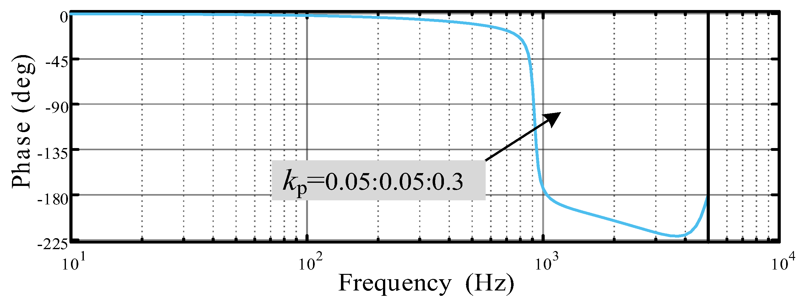
It is evident from Figure 4 that the range of K_p values that maintain system stability is [0, 0.289]. Concurrently, to ensure the system has a certain stability margin, the control system typically necessitates a phase margin of 30 to 60 degrees and a gain margin of greater than or equal to 6 dB. When K_p = 0.14, the open-loop Bode plot of the control system, as shown in Figure 5 and Figure 6, can be obtained, where this parameter provides a gain margin of 6.11 dB and an infinite phase margin.

3.1.2. Resonant Controller Coefficient K_r Design

For resonant controllers, the resonant point causes a phase jump of plus or minus 90 degrees, which complicates the analysis of system stability in the frequency domain. During the design process, the resonant controller coefficient $K_r$ should be determined based on the known proportional coefficient, drawing on $K_r$’s parameter root locus to find the range of K_r values that maintain system stability.

The characteristic equation of the system’s closed-loop continuous transfer function is obtained from the system’s continuous open-loop transfer function, as follows:

$$1+G_{pr}\left(s\right)P\left(s\right)=1+\left(K_p+\frac{K_{r}s}{s^2+w^2}\right)\left(\frac{s{C}_f{R}_d+1}{s^{2}LC+sC\left(R_d+R_f\right)+1}\right)$$

(10)

According to the definition of the parameter root locus, it can be equivalently treated as a unit feedback system, and the equivalent open-loop transfer function expression is:

$$B\left(s\right)=\frac{K_r·s·(Cf·Rd·s+1)}{kp·(s2+\omega 2)·(Cf·Rd·s+1)+(s2+\omega 2)·(Cf·Lf·s2+Cf·s·(Rd+Rf)+1)+1}$$

(11)

Using the inverter parameters presented in Table 1 and by applying the “ZOH” discretization method, the discrete transfer function B(s) is derived as follows:

$$B\left(z\right)=\frac{K_r\left(4.533e-06z^4+7.556e-06z^3-1.511e-06z^2-7.556e-06z-3.022e-06\right)}{z^4-3.66z^3+5.287z^2-3.593z+0.9664}$$

(12)

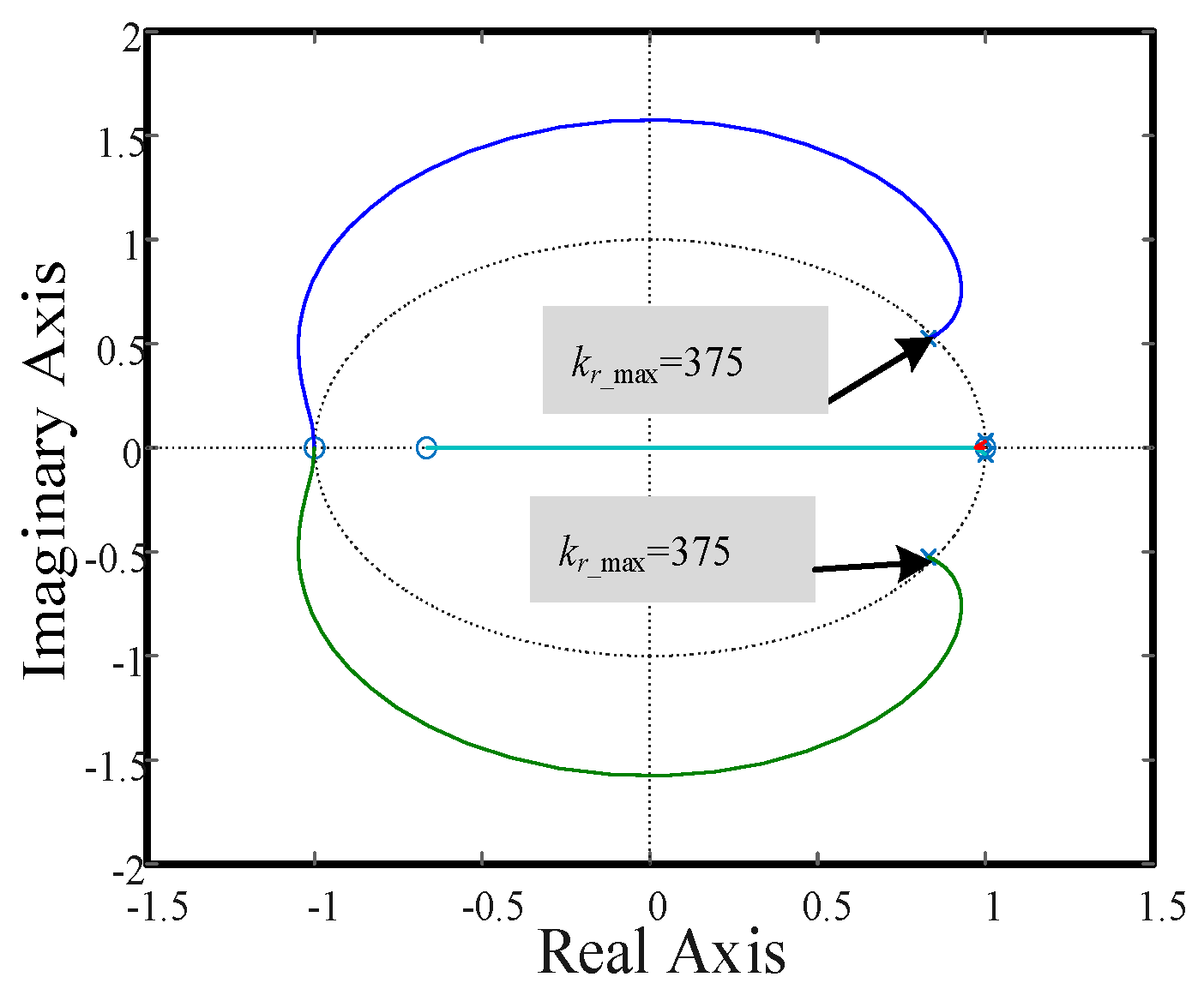
This yields the root locus of the K_r changes, as shown in Figure 7.

From Figure 7, it can be seen that K_r can range from 0 to 375, but specific values still require further analysis. Figure 8 and Figure 9 show the open-loop Bode plot of the system for different K_r values. As K_r increases, the system’s response becomes faster but less stable, also increasing the resonance peaks at the cutoff frequency of the LC filter. In consideration of potential delays and uncertainties in the LC parameters in the actual system, K_r = 300 is chosen, balancing system stability and the transient response requirements, and providing robustness.

3.2. Repetitive Controller Design

The design parameters for repetitive control include the auxiliary compensator Q(z), the compensator S(z), the phase lag compensation coefficient k, and the proportional gain k_r.

3.2.1. Design of Q(z)

Q(z) is a key parameter used to enhance system stability and achieve zero steady-state error tracking. Q(z) is typically set at slightly less than 1, either as a constant or a low-pass filter. As Q(z) approaches 1, the system’s steady-state error decreases and its harmonic suppression capability increases, but it may cause the trajectory of H(z) to lie outside the unit circle at high frequencies, leading to system instability. A comparison of the constant and low-pass filter methods, although a low-pass filter can enhance system stability, shows that it may lose some ability to suppress harmonics at mid–high frequencies and increase the complexity of the control system design. To simplify the design, a constant method is used, and based on analysis by [23], Q(z) = 0.95 is chosen to improve system robustness.

3.2.2. Design of the Compensator Segment S(z)

The design of the compensator segment S(z) typically involves a combination of low-pass and notch filters. When the cutoff frequency of the low-pass filter is slightly below the LC resonance frequency, it can somewhat suppress resonance peaks and rapidly attenuate at high frequencies. It is known that the LC resonance frequency is approximately 973 Hz, as such a second-order Butterworth low-pass filter with a cutoff frequency of 1 kHz is designed, and its discrete transfer function using the “ZOH” method is:

$$S_1\left(z\right)=\frac{0.06746z^2+0.1349z+0.06746}{z^2-1.143z+0.4128}$$

(13)

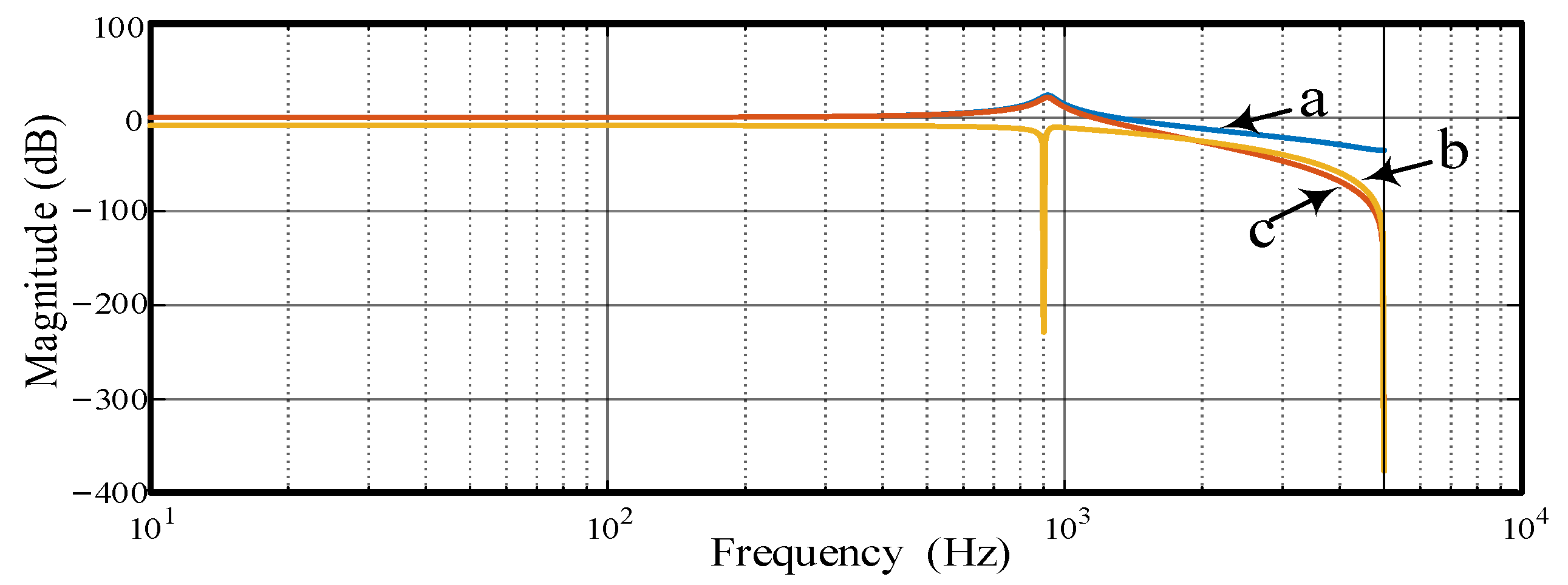
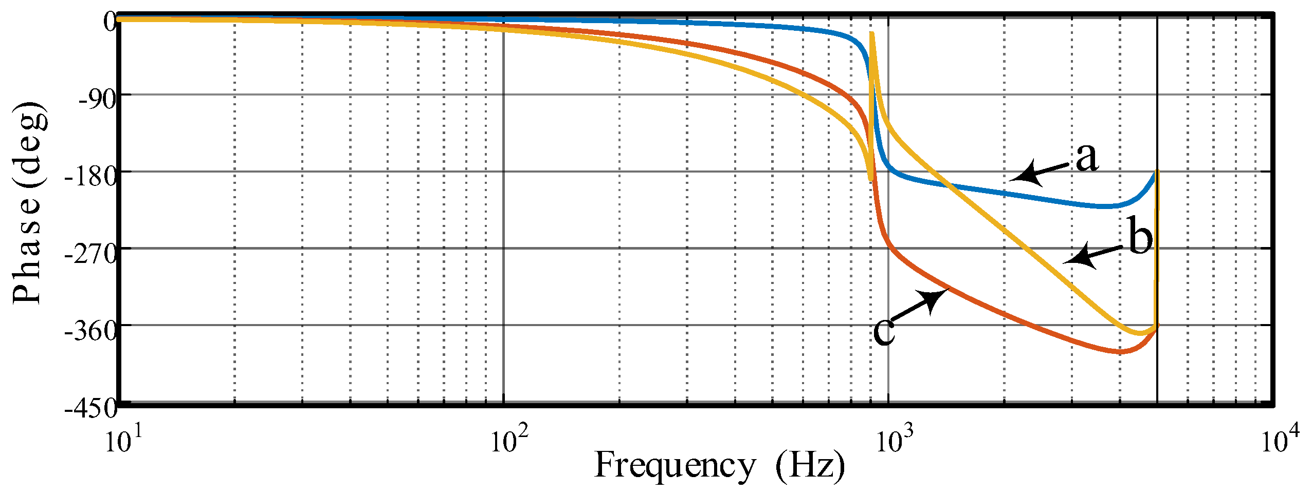
As shown in Figure 10 and Figure 11, the Bode plot before and after compensation of the controlled object P₀(z) is presented. From a comparison of curves a and b, it can be seen that although the low-pass filter suppresses the resonance peak to some extent, the effect is still not ideal. Therefore, a second-order IIR (infinite impulse response) filter is typically used to eliminate the resonance peak without compromising the stability of the system. The basic form of the second-order IIR filter is:

$$\frac{1-2cos\left({\omega }_0\right)z^{-1}+z^{-2}}{1-2r\cos \left({\omega }_0\right)z^{-1}+r^2{z}^{-2}}{S}_2\left(z\right)=\frac{1-2\cos {\omega }_0{z}^{-1}+z^{-2}}{1-2r\cos {\omega }_0{z}^{-1}+r^2{z}^{-2}}$$

(14)

Given that f₀ is the suppression frequency f₀ = 900 Hz, f_s is the sampling frequency f_s = 10 kHz, and the filter radius is r = 0.l, the obtained w₀ = 0.5655. Thus, the designed second-order IIR (infinite impulse response) filter is:

$$S_2\left(z\right)=\frac{z^2-1.6899z+1}{z^2-0.1689z+0.01}$$

(15)

The Bode plot of P₀(z) after compensation with low-pass and notch filters is shown in curve c in Figure 10 and Figure 11. Clearly, under the influence of the notch filter, the system’s resonance peaks are further suppressed, and apart from the fundamental frequency, the system achieves a 0 dB gain requirement at mid–low frequencies.

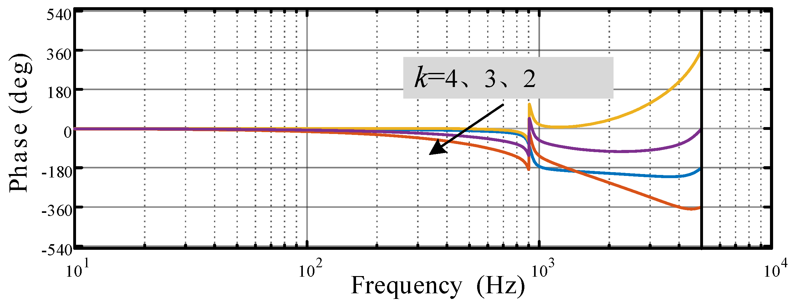
3.2.3. Phase Compensation Segment z^k Design

As seen in Figure 10 and Figure 11, excluding the vicinity of the fundamental frequency, there is a noticeable phase shift in the low-frequency range due to the inherent phase lag of P₀(z) and the increased lag caused by the fourth-order Butterworth filter. To improve the system’s phase–frequency characteristics, a lead segment z^k is introduced, which provides phase compensation for the system. As shown in Figure 12 and Figure 13, choosing k = 2 allows the system to approach a zero phase over a wider frequency range, providing harmonic compensation capability within a 1 kHz range.

3.2.4. Design of Proportional Gain k_r

The proportional gain k_r of repetitive control affects the response speed of the control system and its ability to suppress harmonics. Choosing an appropriate k_r value significantly impacts system stability. After determining the phase compensation k value, the range for k_r is established. The trajectory for different k_r values is shown in Figure 14.

In Figure 14, the system is on the verge of critical stability near the fundamental frequency, caused by the ±90-degree phase jump in the proportional-resonant controller at the fundamental frequency. However, when repetitive control is individually designed, P_o(s) at the fundamental frequency has an infinitesimally small gain amplitude. When Q(z) = 0.95, theoretically, no matter the k_r value, the system can remain stable near the fundamental frequency. Also, as k_r increases, the system stability decreases, but the error convergence speed and harmonic suppression capability improve. Considering potential the delays in control and the uncertainties in system modeling, a conservative k_r value is chosen; this paper selects k_r = 2.

3.3. Inertia Parameter k_vw Design

When designing the frequency–voltage coefficient, the voltage stress on the capacitor and the capacitance size must be considered. In this paper, the maximum tolerable DC voltage is selected to be 1.5 times the rated voltage. Therefore, V_{dc_max} = 800 × 1.5 = 1200. Based on the V_{dc_max}, the maximum value of the frequency–voltage droop coefficient can be determined. For frequency variations within ±0.5 Hz, the virtual inertia element is activated. When the frequency deviation exceeds ±0.5 Hz, the grid frequency is considered to be over/under frequency, and the virtual inertia element is not activated. To ensure the longevity of the DC capacitor, a conservative k_vw = 180 V/Hz is selected. When the grid frequency fluctuates by 0.5 Hz, the maximum change in the system output voltage is 90 V. The larger the k_vw, the greater the virtual inertia of the APF, and the better the transient support for the grid; conversely, the smaller the k_vw, the smaller the virtual inertia of the APF, and the worse the transient support for the grid. With this step, the parameter design process is complete. The

Table 2. APF system control parameters.

Parameter	Value
Kp	0.14
Kr	300
Q(z)	0.95
kr	2
m	2
kvw	180

below presents the system control parameters:

4. Experimental Platform Introduction and Results

4.1. Experimental Platform Introduction

The experimental platform consists of three parts: (1) a simulated grid, namely a virtual synchronous machine is used as the simulated grid in this paper; (2) resistive load and rectifier-type nonlinear load; and (3) 10 kVA APF equipment. The wiring is shown in Figure 15:

Figure 16 shows a photograph of the experimental prototype. The experiment uses ModelingTech MT 3200 HIL (Made in China) to simulate the main circuit, with the control part using 10 kVA PCS1 and 10 kVA PCS2 control boards to implement the control algorithms for both the VSG and the APF. Host computer 1 is connected to the 10 kVA PCS in order to send related commands, and host computer 2 is connected to the MT 3200 HIL to capture experimental waveforms and import them into Matlab/Simulink (2023a) for further analysis.

4.2. Experiment Results

• Rep1: Without APF harmonic suppression
• Rep2: Verification of APF harmonic suppression effect with PI control
• Rep3: Verification of APF harmonic suppression effect with PR + RC control

Figure 17 and Figure 20a,b show the grid voltage and current waveforms without APF harmonic mitigation. The voltage and current waveforms are severely distorted, with the voltage THD reaching 6.39% and the current THD reaching 10.3%. Figure 18 and Figure 20c,d display the grid voltage, current, and harmonic current waveforms when the APF with PI control is applied for harmonic mitigation. It can be observed that there is a slight improvement in the voltage and current waveforms, although some distortion remains, with voltage and current THD values of 3.96% and 4.83%, respectively. Figure 19 and Figure 20e,f illustrate the grid voltage, current, and harmonic current waveforms when the APF with composite repetitive control is implemented for harmonic mitigation. The voltage and current waveforms show no visible distortion, with THD values for the voltage and current reduced to 3.71% and 3.57%, respectively. Harmonic suppression is visible in the spectrum, with THD values reduced by 0.25% and 1.26% compared to PI control. Specifically, the grid voltage THD decreased by 6%, and the grid current THD decreased by 27%. The superior performance of composite control is evident.

• Rep4: Verification of transient frequency support effect under grid frequency variations

As observed in Figure 21a, the maximum frequency droop without using the proposed method is approximately 49.57 Hz. In contrast, when the frequency controller is activated, the maximum frequency droop can be limited to 49.6 Hz. Therefore, the proposed virtual inertia method reduces the frequency deviation by 17%. Additionally, another critical parameter is the RoCoF, which can be reduced from 1.8 Hz/s to 1.5 Hz/s, indicating a 17% improvement over the case without virtual inertia. With the proposed method, the RoCoF is determined by the combined inertia of the APF and the power system and can be flexibly designed by changing the virtual inertia coefficient k_vw. As shown in Figure 21b, the quasi-steady-state voltage deviation is approximately 72 V, and the corresponding voltage deviation is within the maximum allowable voltage deviation of 90 V. Furthermore, Figure 21c,d demonstrates the energy and power output of the APF during frequency dynamics. As shown in Figure 21c, the APF produces energy during the frequency event to provide frequency support. Furthermore, it is clear from Figure 21d that the proposed method does not interfere with the normal operation of the APF, as the output power remains at zero in a quasi-steady state.

5. Conclusions

This research proposes a concept for grid-connected APFs to generate distributed virtual inertia and utilizes composite repetitive control to mitigate harmonics. This approach can effectively increase power system inertia, reduce frequency deviations, and decrease the rate of change of grid frequency under large disturbances, while further suppressing harmonics. The virtual inertia is emulated by DC-link capacitors in grid-connected APFs without increasing system cost and complexity. By using the grid frequency as a common signal, APFs can easily adjust the DC-link voltage proportionally. Consequently, all the DC-link capacitors are aggregated into an extremely large equivalent capacitor for frequency support. Furthermore, the design parameters of virtual inertia, including DC-link capacitance, DC-link voltage, and maximum DC-link voltage deviation, have been identified. The experimental results indicate that the proposed concept can achieve a 17% reduction in frequency deviation, a 17% improvement in the RoCoF, and a 6% and 27% improvement in the voltage and current THD, respectively.