1. Introduction
A traditional grid structure includes large power plant generation stations, high-voltage transmission lines, and distribution stations. This kind of electric power system can be considered one of the greatest engineering achievements of mankind. This success is due to the invention, development, and deployment of synchronous generators such as coal gas, hydro-, and nuclear power plants [
1]. However, large power plant stations utilize mainly fossil fuels for power generation, and the power transmission lines result in high losses. These power plants are being increasingly retired because of concerns about climate change and the CO2 emissions generated by fossil fuels. In addition, the International Renewable Energy Agency’s roadmap for increasing solar and wind power generation from 30% to 85% by 2050 [
2] points out the future of renewable energy. The global integrated PV capacity reached almost 800 gigawatts in 2020 [
3], and private companies have been investing in the research and development of renewable energies [
4]. As a result of these progressions, it can be claimed that renewable energy systems will be widely used in the next two decades in residential and commercial buildings.
However, some renewable energy systems do not include an energy storage system, instead using only PV cells and a grid [
5]. The main limitation of such systems is that they are not able to provide power to the load in the case of grid failure because the DC-AC inverter will shut itself down. In addition, the load is not supplied at night and the excess power during the day is not stored. Moreover, such systems usually involve grid-following (GFL) inverters; however, it is not ideal to have too many GFL inverters because, when the penetration of GFL inverters increases, the frequency nadir reduces. On the other hand, even though some systems include PVs, a grid, and energy storage systems, their power levels are low and they include simulation results [
6,
7,
8], whereas our setup at the FSEC is a huge system and the measurements were taken from a real-world setting that was used for two years.
A microgrid can be a self-sufficient electric power system that has an islanding ability. A microgrid that has intelligent subsystems can also be connected to the grid. One of the challenges of a microgrid that is connected to the main grid is the use of grid-forming (GFM) inverters. This is because synchronous generators are coordinated to a single frequency (60 Hz in the USA) to act in harmony, and these power plants are called grid-forming power plants. GFM inverters act as a voltage source. This is important for forming and maintaining a healthy grid; however, GFL inverters presume that the grid is currently formed and maintained under good conditions, so they can be considered current sources [
9]. Other challenges include the integration and design of a power management control system to enable renewable energy system integration. As a result of this, after testing the integrated high-power inverter and high-energy battery storage systems, the next step is to add PV panels into the existing system using a three-port bidirectional inverter [
10,
11] for microgrid applications. The main contributions of this research include the application of load shifting through the creation of a power management control algorithm and the implementation of peak shaving and an even energy consumption. This will allow demand charges to be avoided by optimizing the PV panel capacity at the FSEC.
An overview of this integrated system is given in
Section 2 of this paper. It is also a good approach to discuss what the ride-through requirements are when either a renewable energy source or a battery energy storage system is connected to the grid. These requirements are pointed out in
Section 3. Next, depending on the power management algorithm, the test results and scenarios are discussed in
Section 4.
Section 5 explains the methodologies that were utilized. The testing results, the simulation outcomes, and an analysis of the system are presented in
Section 6. The conclusions and future work are summarized in
Section 7.
2. Integrated System Overview
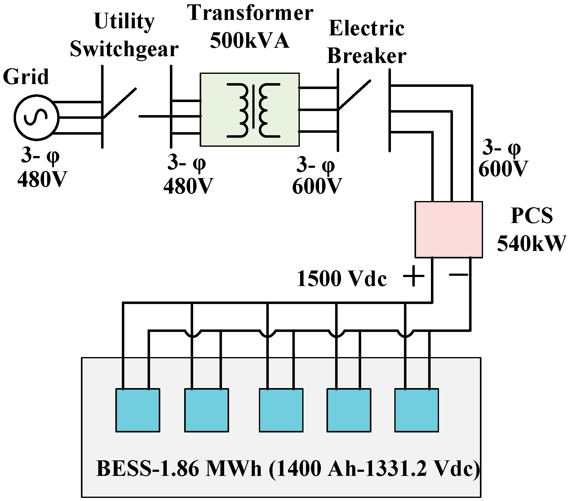
The system’s test setup consisted of five main parts, as shown by the block diagram in
Figure 1. These parts were the utility switchgear, a transformer, an electric circuit breaker, a three-phase bidirectional inverter, and a battery energy storage system that included five lithium-ion battery pods. The utility switchgear had a three-phase 480 VAC output, and it was connected to the three-phase transformer as an input. The transformer was a step-up transformer whose output was a three-phase 600 VAC, and its power was 500 KVA. It was connected to the breaker before the power conversion system (PCS).
2.1. Power Conversion System
The PCS used a 540 KVA Dots Energy bidirectional three-phase AC-to-DC inverter system that consisted of three main parts: an auxiliary power supply, inverters, and a DC combiner, as shown in
Figure 2. The auxiliary supply used 3 KVA of power and comprised a single-phase 240 VAC system for the main controller, the cooler for the BESS, and the communication system. In the PCS, there were three 180 KVA bidirectional inverters in parallel whose inputs were three-phase 600 VAC. The output of the inverters was 1500 VDC, a nominal 200 amps, and a maximum of 600 amps. The DC combiner combined the DC outputs that were generated by the inverters.
2.2. Battery Energy Storage System
The battery energy storage system (BESS) from the Contemporary Amperex Technology Company Limited (CATL) had a total capacity of 1400 Ah (1.86 MWh) and five battery pods in parallel. Each pod had a nominal voltage of 1331.2 VDC and eight battery modules in series, and the battery modules had lithium iron phosphate cells. Each battery module had one local battery management system (BMS), each pod had one master BMS, and the BESS was connected to the main BMS in the PCS.
3. Ride-Through Requirements in Grid Connection
Conventional AC power systems are dominated by synchronous generators (SGs). These systems have a high inertia, behave almost as an ideal voltage source, and provide a stable frequency [
12,
13,
14], which are essential features for maintaining a highly regulated power grid. Moreover, the current-handling capabilities of SGs are typically up to six times the rated currents. The primary control objectives of SGs are voltage and frequency regulation, which are achieved through exciter and governor control.
Renewable energy sources that might include battery energy storage systems are intermittent, and they have issues involving a low inertia. This means that renewable energy systems cannot store kinetic energy in the same way that AC power systems can. As a result, they are more sensitive to sudden changes in the load or generation. One of the biggest challenges posed by low inertia is the risk of cascading failures.
Therefore, the primary objective of GFL inverters is to deliver active power. Supporting the grid is the secondary objective. However, the first objective of GFM inverters is to regulate the voltage and frequency of the grid by changing the active and reactive power references continuously. Based on the properties of synchronous generators, GFM inverters should support load sharing/drooping, black starts, inertial responses, and hierarchical frequency/voltage regulation [
15,
16,
17]. Moreover, there are basic requirements for grid connections regardless of whether GFL or GFM inverters are utilized.
Ride-through is defined as the capability of an electrical system to maintain its connection over short periods when the electric network’s voltage or frequency changes. The ride-through requirements are defined by the grid connection standards [
18,
19]; these include the California Rule 21 and IEEE standards 1547-2018, which are shown in
Table 1 and
Table 2.
For the frequency requirements, both GFL and GFM inverters must be disconnected from the grid immediately if the frequency exceeds 66 Hz or falls below 50 Hz. When the frequency is in over-frequency region II (61.8 Hz to 66 Hz) or low-frequency region II (50 Hz to 57 Hz), the circuit breaker should trip in 0.16 s. While in over-frequency region I (61.2 Hz to 61.8 Hz) or low-frequency region II (57 Hz to 58.8 Hz), the inverters can maintain their connections to the grid for up to 299 s.
For over-voltage region II, the inverters must be disconnected from the grid in 0.16 s when the voltage exceeds 120 V (in the USA). If the voltage value is between 110 V and 120 V, the connection should be tripped in 12 s. For low voltages, there are three regions. The inverters can remain connected for up to 20 s, 10 s, or 1 s if the voltage levels are between 70 V and 88 V, between 50 V and 70 V, or below 50 V, respectively.
These requirements originated from grid-connected GFL inverters. The implementation of these requirements for GFM inverters is also valid in the grid-connected mode.
4. Power Management Algorithm and Scenarios
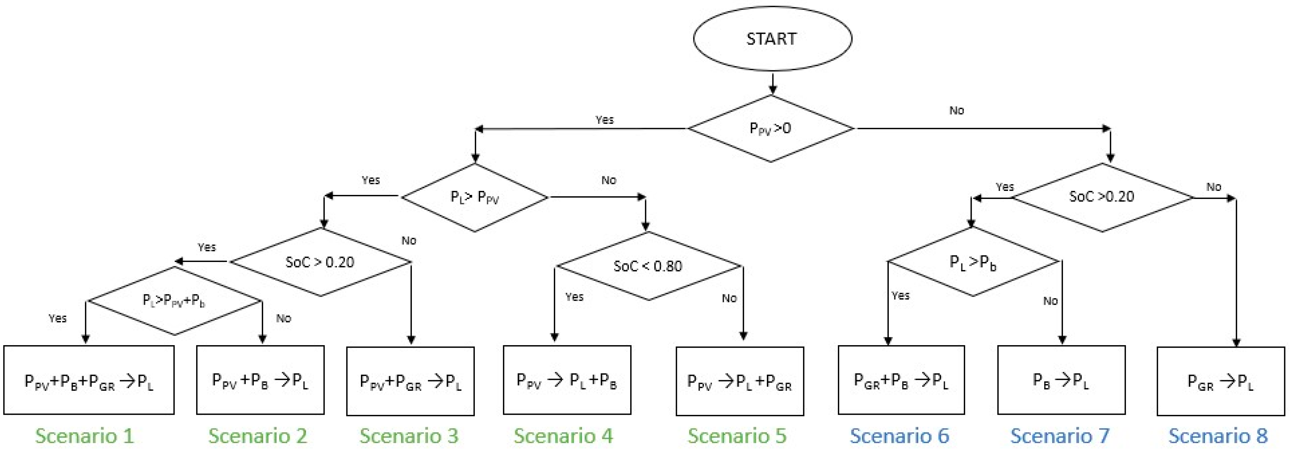
In this section, eight different power management scenarios are discussed. As shown in
Figure 3, the first five scenarios included the power generated by PV panels. However, Scenarios 6, 7, and 8 were not dependent on PV panels. Based on all the scenarios, it was clear that the PV panels acted as a power source and the load was a load. On the other hand, the battery and the grid can be power sources or loads depending on the scenario. Each scenario is examined in this section.
4.1. Scenario 1: All-Sources Mode
All the power flow scenarios started with checking the power of the PV panels to determine its availability. If this power was available, then the scenario checked how much power the load needed. Then, it examined whether the power from the PV panels was enough for the load. If the PV panels’ power was not enough, the scenario checked the BESS power. If the load power was not satisfied by the power of both the BESS and the PV panels, the remaining power was obtained from the grid in this scenario. This is why all the power sources were combined to meet the load power demand.
4.2. Scenario 2: DC2Load Mode
In this scenario, after checking the power of the PV panels and the BESS’ state of charge in order to estimate whether the load demand can be handled, the power from the grid was not needed. In addition, the PV panels and BESS had the same DC link bus, and they provided AC voltage to the load by converting their DC voltage to AC voltage.
4.3. Scenario 3: PV + GRID Mode
If the PV panels produced power, but this power was not enough and the BESS did not have sufficient energy for the load, the power from the PV panels and the grid were utilized. Therefore, this scenario is called the PV-plus-grid mode.
4.4. Scenario 4: Sunshine Mode
In this scenario, when the sun was shining, the PV panels supplied adequate power to the load and the excess power from the PV panels was sent to the BESS if the SoC of the BESS was less than 0.8 in order to charge it. Thus, DC voltage from the PV panels was converted to DC voltage for the BESS, and it was then converted to AC voltage for the load.
4.5. Scenario 5: DC2AC Mode
The recognized steps include checking the power of the PV panels first, and then checking the SoC of the BESS. In this scenario, when the PV power satisfied the load power and the SoC of the BESS was full, the surplus power was sent to the grid.
4.6. Scenario 6: BESS + GRID Mode
In this scenario, the PV panels did not supply any power. Therefore, the load needed to obtain power from the grid and the BESS. Load shifting was performed in this scenario.
4.7. Scenario 7: BESS Mode
In this scenario, the load power was covered fully by the BESS, and the number of hours for which the BESS can supply power until the grid is necessary was determined. This mode helped to determine the size of the BESS when the whole system moved towards disconnecting from the grid.
4.8. Scenario 8: GRID Mode
This scenario provides the load profile and energy usage of the system when the PV panels and the BESS do not exist because the load demand is satisfied by the grid.
5. Methodology
5.1. Optimal Cost, BESS, and PV
The optimal battery size can be different depending on each case study, and the case studies were also very similar to each other, as mentioned in References [
20,
21,
22]. However, in this model, the following equations [
23] were utilized for two cases. In the first case, the BESS’s capacity size and the PV panels’ power size were determined based on the building energy consumption and solar irradiance of the location. In the second case, the size of the PV panels was determined depending on the BESS already located at the FSEC.
The total power generated,
, by solar power (
) is given in Equation (1).
For a given average load power of
with inverter and battery efficiencies of
and
, respectively, the required present average battery power,
can be determined using Equation (2), where
represents the prior average battery power.
If we define the total minimum and maximum battery pack energies as
and
, respectively, then their values are limited by the minimum and maximum
SoC, as follows in Equations (3) and (4).
Then, our charging algorithm will guarantee that the nominal stored battery energy
is governed by Equation (5).
When the power generated from the
PV panels and the power stored in the battery pack are not enough to cover the load power at a given time
t, the power loss (
PL) is defined by Equation (6).
Then, the power loss probability (PLoP) is defined as the ratio of the total power loss to the total load power; it is expressed in Equation (7).
5.2. Load Shifting
The idea of load shifting is to reduce the energy usage or load demand during the peak demand hours and to move that energy usage to off-peak hours [
24]. Basically, using energy storage systems during on-peak hours and charging them during off-peak hours makes the energy usage more uniform [
25]. In this process, the total energy consumption does not change, but it helps to avoid extra charges by the utility [
26]. Even though the on-peak hours can depend on the season, the on-peak and off-peak hours can be defined as shown in Equation (8):
Then, depending on the time, the energy storage systems can be a load or a supply. The function of the load demand is defined in Equation (9), where
is the load demand power at time
t,
is the power supplied by the grid at time
t, and
is the battery-load power or the battery-supply power at time
t:
5.3. Peak Shaving
Peak shaving is the process of reducing the power consumption during periods of high demand [
27] by using usually renewable energy sources. In contrast to the load-shifting objectives, the peak shaving process reduces the total energy consumption of the grid.
Two methods of peak shaving [
28] are illustrated in
Figure 4 and
Figure 5. One of the popular techniques is called the fixed-demand method, in which the BMS executes a command to charge at a lower demand limit and to discharge at an upper demand limit. Another technique is the fixed-threshold method. In the fixed-threshold method, when the load demand is higher than the threshold limit, the BESS is discharged. When the load demand is less than the threshold limit, the BESS is charged.
6. Results and Discussion
In this section of the article, the simulation and test results and measurements are presented and discussed. The first test was the factory acceptance test (FAT). The battery pods were charged and discharged according to the manufacturer’s parameters. When this test was performed, the results were sent to the company via the BMS. Then, the company confirmed whether the battery pods were safe to operate. Next, we tested the scenarios by starting from scenario 8, because it was important to determine the load profile first. Therefore, the scenarios are presented in descending order in this section. In this section, after all the calculations were performed, the following efficiencies were considered: 92% for the PCS and 98% and 97% for the BESS during charging and discharging, respectively.
6.1. Battery Safety Testing Results
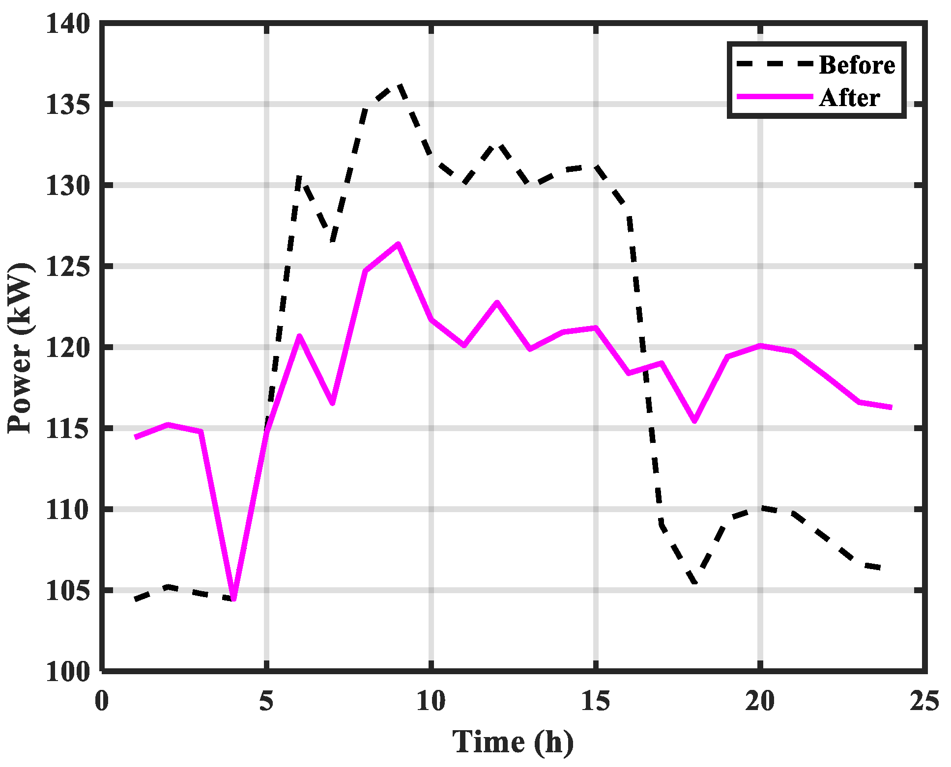
First, the FAT was performed on the batteries. This test was conducted according to the FAT requirements from the CATL company as follows: start at a 40% SoC (state-of-charge), then discharge the batteries to a 0% SoC. After that, charge them to a 100% SoC and discharge them to a 0% SoC. Again, charge them to a 100% SoC and discharge them to a 40% SoC.
Figure 6 illustrates the power usage of the FSEC during the test.
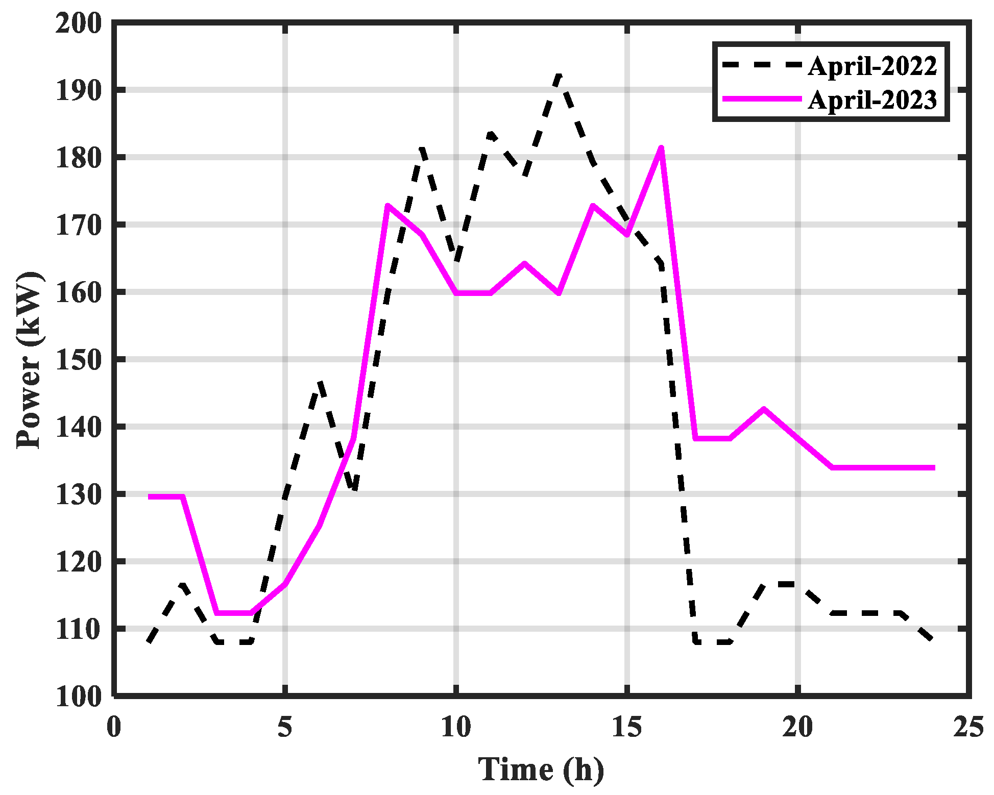
Figure 7 shows the power usage from the grid during the second BESS test, which was conducted in order to determine how the FAT is performed in a real-world setting.
The SoC of the second battery pod in the BESS is plotted in
Figure 8. The reason for this test was to ensure that all the BMSs in the BESS were working properly. In addition, it is crucial to confirm that the voltages of all the battery cells are within the desired limit, and that the cooling system functions as programmed. The thermal management technique for the BESS was a liquid cooling management system.
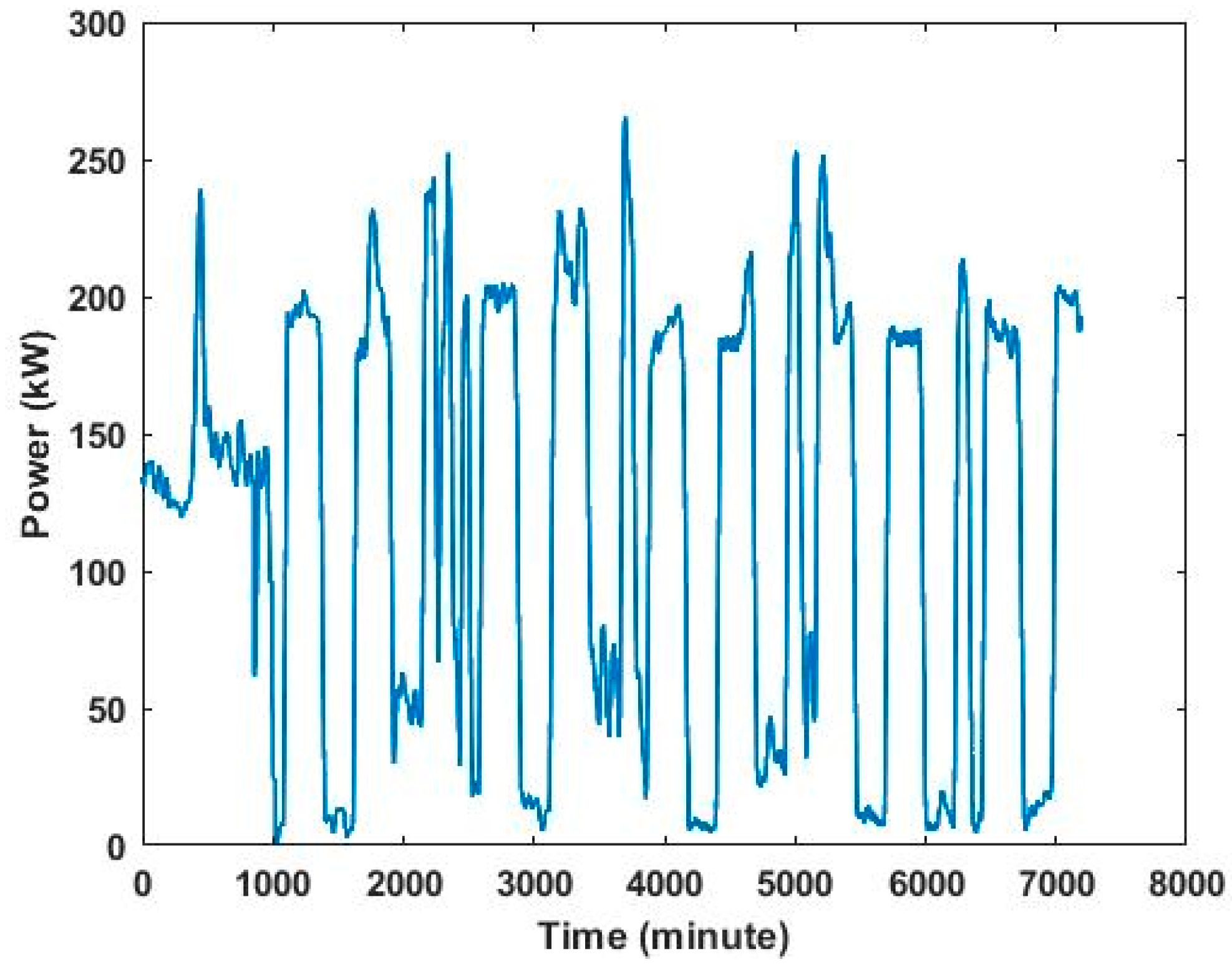
6.2. Scenario 8 Testing Results
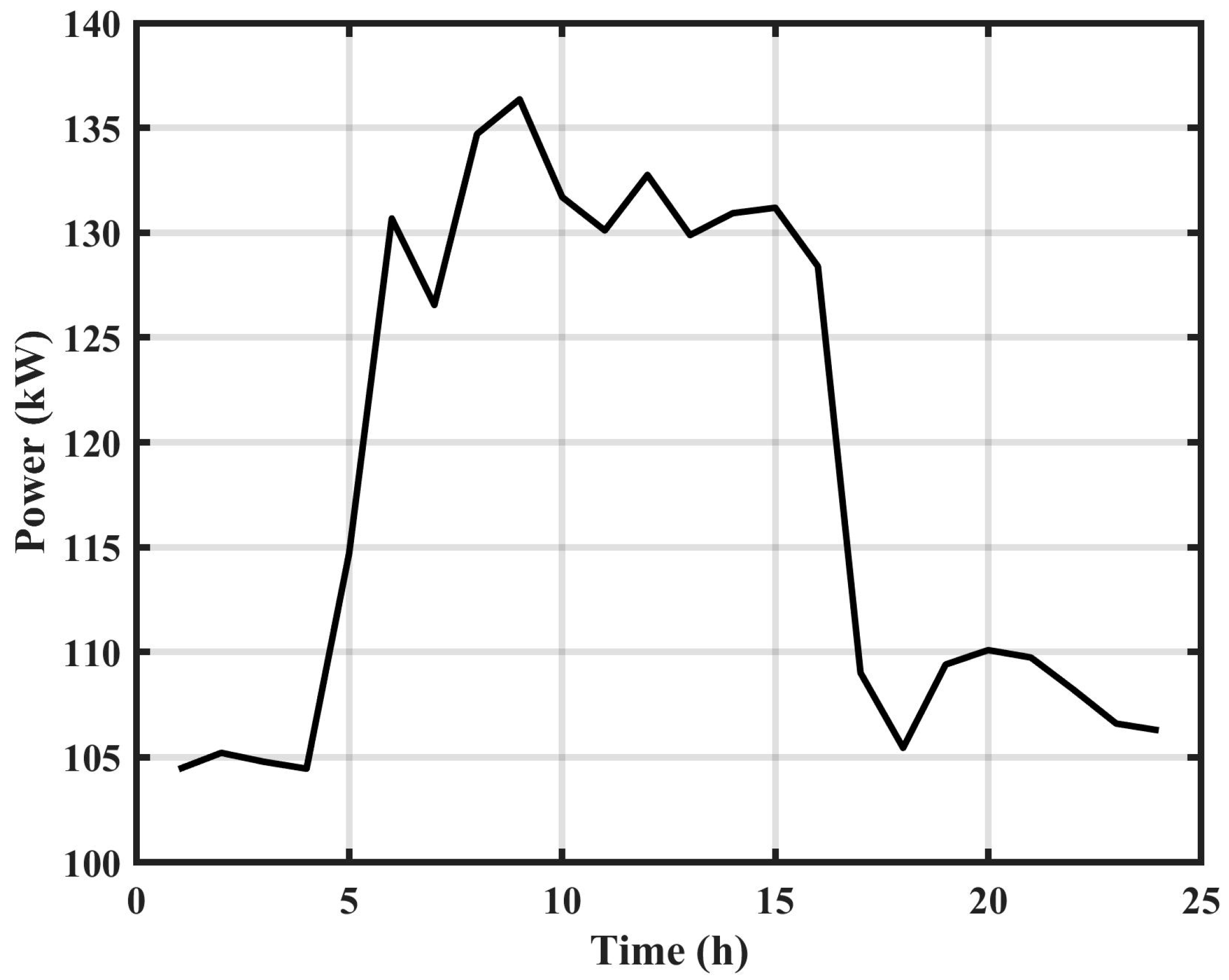
After the FAT, the next test involved executing the GRID mode scenario. This test helped us visualize the energy usage of the FSEC building before the integration. In addition, it can help determine how many PV panels are needed, how much peak shaving can be implemented, and how much battery capacity is needed for islanding in a microgrid. The FSEC’s average power usage in 2021 is illustrated in
Figure 9.
The integration of this system started in the first quarter of 2022, and many tests were performed from time to time. During these tests, the power from the grid was utilized excessively. We chose not to provide the average power usage for 2022 because it might not accurately reflect the energy usage of the FSEC building. Therefore, the load profile of the FSEC in 2021 is provided.
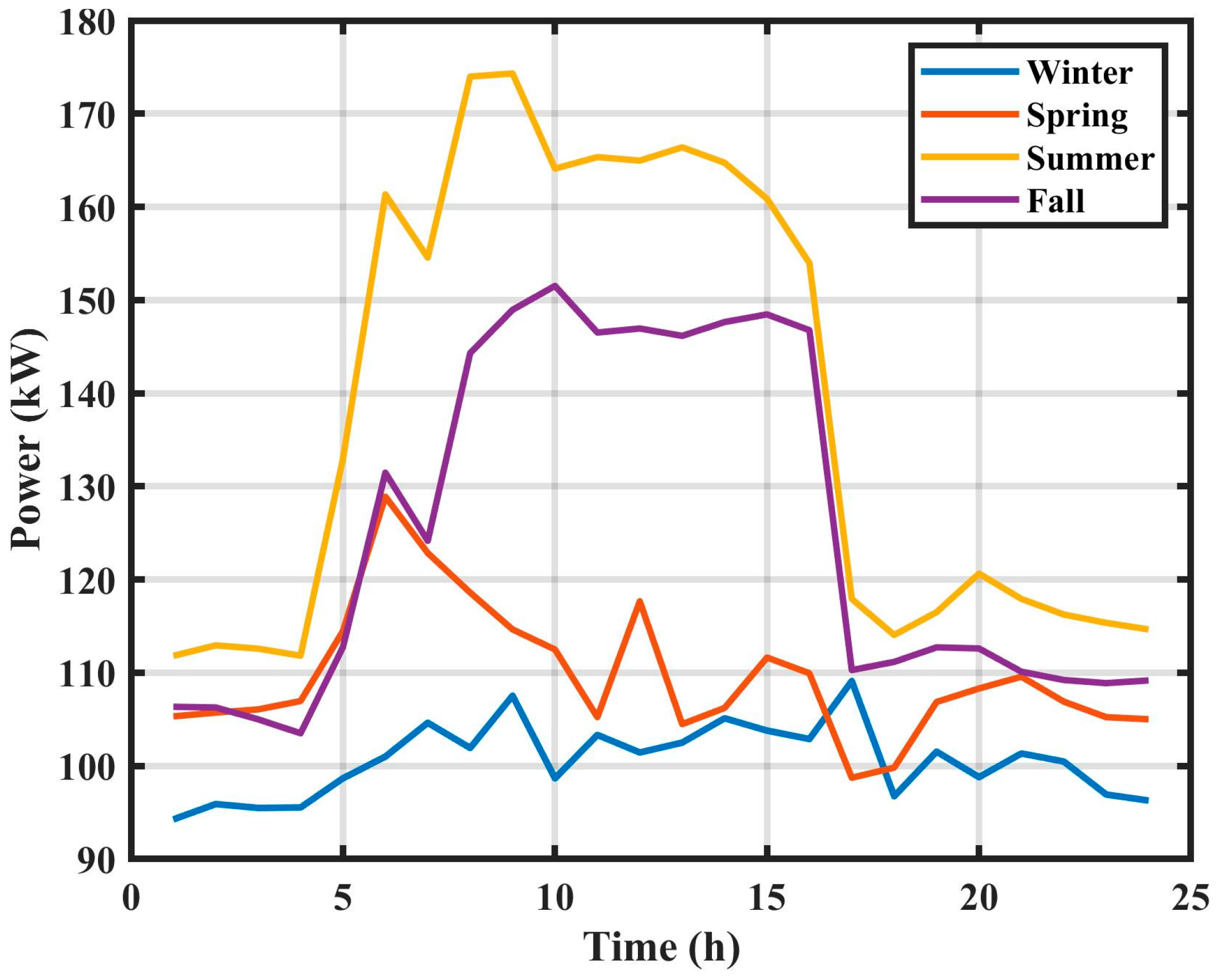
Figure 10 explains the energy usage of the FSEC during each season. The usage was 2414 kWh, 2632 kWh, 3320 kWh, and 3001 kWh in the winter, spring, summer, and fall seasons, respectively.
It was also realized that the energy usage in the summer and fall was due to the hot weather in Florida and the usage of air conditioning, but the solar irradiance of those seasons is also higher, as shown in
Figure 11.
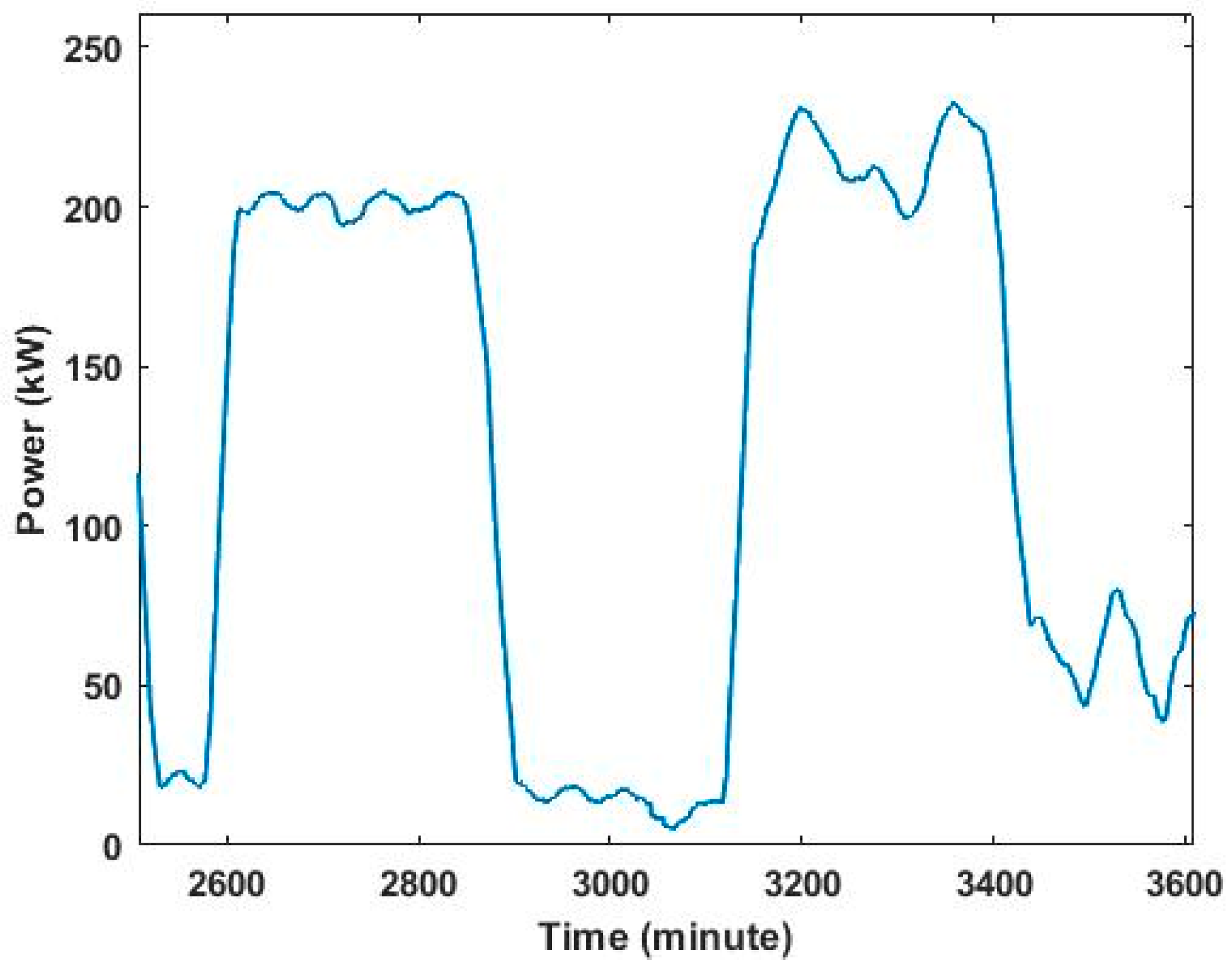
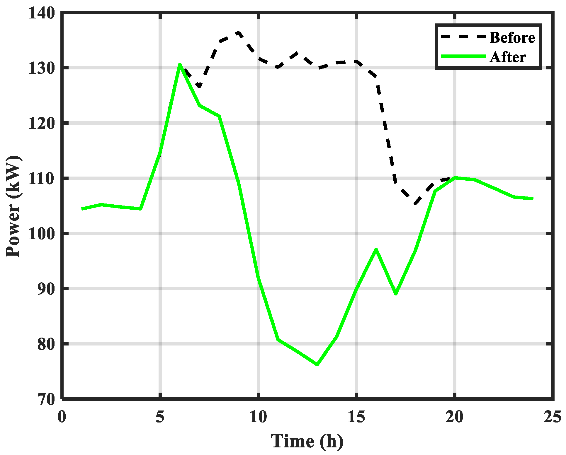
6.3. Scenario 7 Testing Results
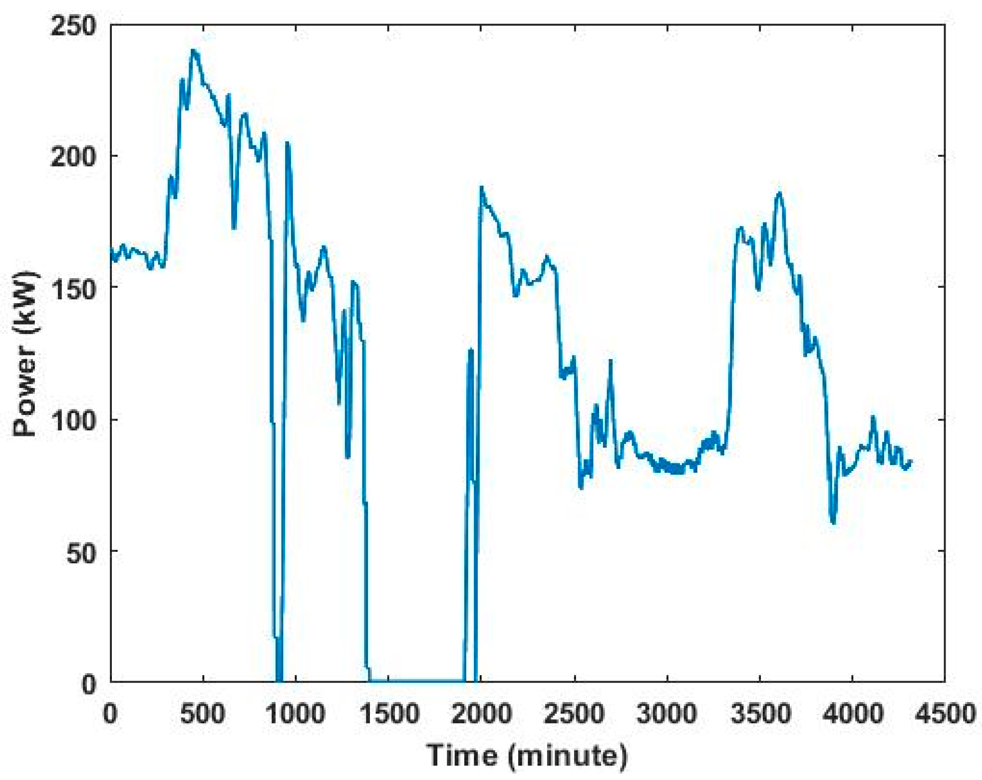
The BESS mode allowed us to observe for how many hours the FSEC experienced zero power usage from the grid while discharging the BESS. As shown in
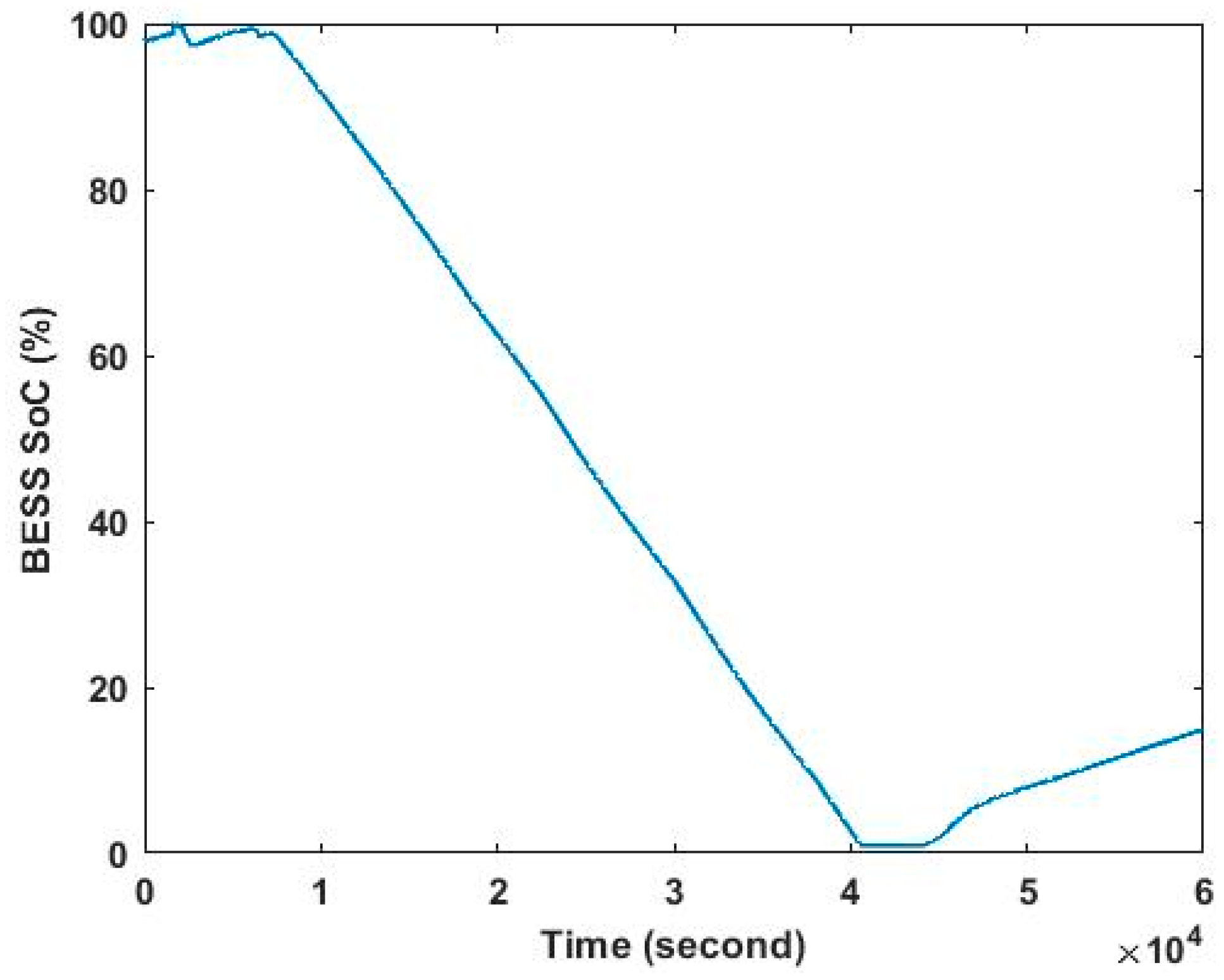
Figure 12, the power usage of the FSEC was simulated for three days.
Figure 13 illustrates the SoC of the BESS during this scenario. As a result of this scenario, the energy usage of the FSEC from the grid became zero for more than 9 h. The reason that the FSEC power usage is in minutes is because the data were taken from the utility, which measured the power usage every minute. However, the SoC data were taken from the BMS in the BESS, which checked the SoC of the batteries every second.
6.4. Scenario 6 Testing Results
Load shifting was performed in Scenario 6 using the BESS + GRID mode. In this simulation, 110 kWh of energy used from the battery pods between 6 AM and 4 PM was shifted to the time period between 5 PM and 3 AM, as plotted in
Figure 14 based on the average power usage for one year.
However, due to the fact that the charging and discharging efficiencies were not equal, and some electrical energy was converted to heat energy, the total number of battery-charging hours was one hour more than the total number of discharging hours in practice. Therefore, 180 kWh of energy utilized from the batteries between 8 AM and 5 PM was shifted to the period between 8 PM and 5 AM for the month of April. These test measurements were performed only on weekdays. It can be seen that the energy consumption during on-peak hours shifted to off-peak hours, as demonstrated in
Figure 15.
6.5. Scenario 1 through 5 Simulation Results
This section includes the first five scenarios. The FSEC has 80 kW power PV panels that were acquired for another research purpose. Now, these PV panels are being integrated into the existing system, and the fixed-threshold method was applied. The expected FSEC power usage profile if these PV panels are utilized is illustrated in
Figure 16.
However, if the BESS with the 80 kW PV farm is used for two goals—peak shaving and the uniformity of power consumption—then, theoretically, a 196 kWh BESS is sufficient to achieve better peak shaving, as seen in
Figure 17. The batteries should not be discharged fully in order to increase their lifespan, and the batteries’ charging/discharging efficiency should also be considered. As a result, a 250 kWh BESS is encouraged.
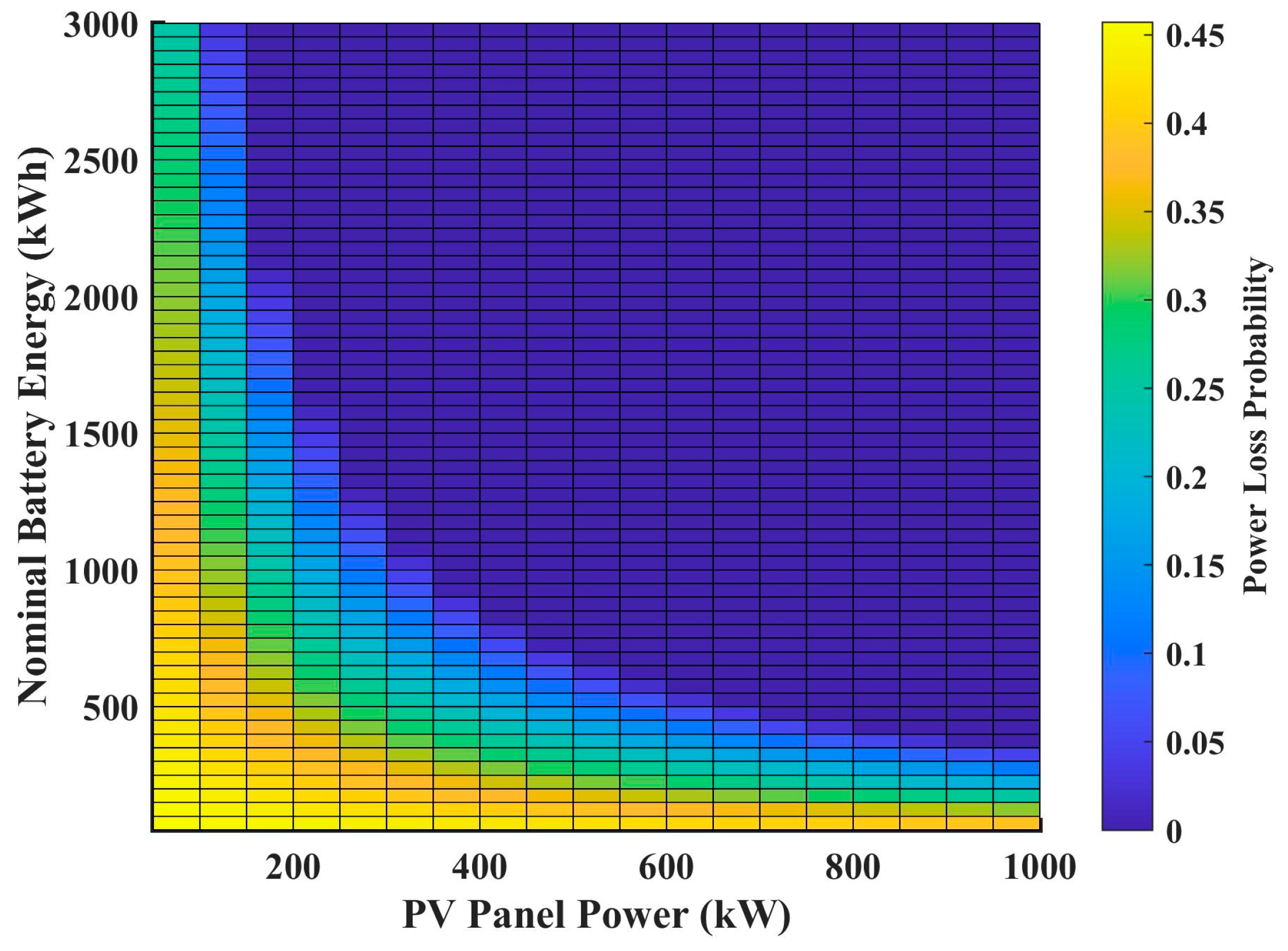
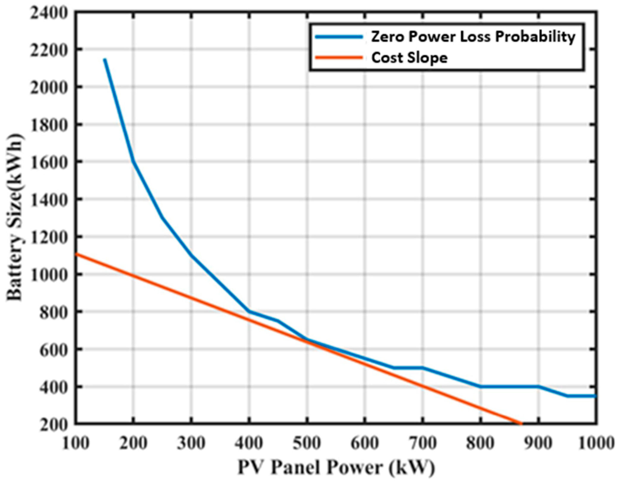
The next goal in this scenario was to increase the BESS size and PV panel size in order to obtain a microgrid with an islanding mode, which allows it to disconnect fully from the grid. As seen in
Figure 18 and
Figure 19, the
PLoP and the optimal sizes of the BESS and PV panels were simulated based on the cost function in [
29] for the FSEC building. Therefore, in order to be off-grid, the optimal BESS energy capacity and PV panels’ power capacity should be 650 kWh and 500 kW, respectively. This also means that a capacity of PV and BESS below these values should not be selected.
6.6. Total Harmonic Distortion (THD) Testing Results
In this test, the data were obtained with an oscilloscope by using current transforms (CTs). The CTs used were high CTs, with the model number SCT-065-800 from EKM Metering Inc., and they provided an output of 26.6 mA when 800 A traveled through the CTs.
The waveforms were obtained at the utility switchgear in order to observe how much the waveforms were distorted before sending them to the grid. The voltage and current waveforms were measured while the BESS was discharged at 200 kW for 10 min and while the BESS was charged at 100 kW for 10 min. The voltage waveforms are shown in
Figure 20 while charging and
Figure 21 during discharging.
At the utility switchgear, the voltage was 480 VAC; then, the RMS current level became 240.56 A for a 200 kW discharge. Theoretically, this 240.56 A current traveled through the CTs, whose outputs were 7.999 mA; then, 799.9 mV must be seen in the oscilloscope when using a 100-ohm resistor, as illustrated in
Figure 22. During the 100 kW BESS charge, the output current became half of that during the discharging scenario, as demonstrated in
Figure 23.
The THD (Total Harmonic Distortion) is a relative measure of the distortion defined through the ratio of the RMS value of the distorted waveform and the RMS value of the fundamental component [
30]. The THD is defined in Equation (10).
During discharging, the average THD value is 7%. However, it is 16% for a 100 kW charging scenario. The reason that the THD level became worse was because the high CTs’ accuracy decreased when the current level decreased.
7. Conclusions
The incorporation of advanced systems at the FSEC through a partnership between the University of Central Florida and A.F. Mensah Inc. includes a bidirectional three-phase inverter with a capacity of 540 KVA and a battery energy storage system with a capacity of 1.86 MWh. The integrated system is currently being used by the FSEC without PV panels. This study provides an overview of this integrated system and a discussion of eight power management scenarios for a microgrid purpose. The energy consumption of the building, the reduced energy consumption, battery testing, load shifting, and peak shaving are presented. Except in the case of peak shaving, the data for the other cases were obtained via real-time measurements (the peak shaving case requires PV panel integration). Firstly, load shifting was achieved by shifting 180 kWh of energy usage from the morning times to night times. Secondly, the peak shaving case was simulated for two cases, with a BESS and without a BESS. An 80 kW PV farm with a 250 kWh BESS was adequate to obtain peak shaving and the uniformity of power consumption. Thirdly, to form a microgrid without a grid, the optimal capacity of the PV panels was determined to be 500 kW. The THD level was determined to be 0.07 in the case where 200 kW of power was sent to the grid. It is crucial to mention that, when more power was sent to the grid, the THD level became better due to the nature of the current transforms. A future step will be to integrate a three-port bidirectional inverter using modular-design, GaN-based switches and PV panels, because the current inverter is a two-port bidirectional inverter.
Author Contributions
Conceptualization, S.G. and I.B.; methodology, S.G.; software, S.G.; validation, S.G. and A.-c.D.; formal analysis, S.G.; investigation, S.G. and A.-c.D.; resources, S.G. and A.M.; data curation, S.G.; writing—original draft preparation, S.G.; writing—review and editing, S.G. and A.-c.D.; visualization, S.G.; supervision, A.M. and I.B.; project administration, A.M. and I.B.; funding acquisition, I.B. All authors have read and agreed to the published version of the manuscript.
Funding
This research was partially funded by A.F. Mensah Inc.
Data Availability Statement
The original contributions presented in the study are included in the article, further inquiries can be directed to the corresponding author/s.
Acknowledgments
Sahin Gullu is affiliated with the Department of Electrical and Electronics Engineering at the Nevsehir Hacibektas Veli University, and he was also sponsored for a study-abroad program by the Ministry of National Education, the Republic of Turkey. MATLAB R2018a was used for simulation and data illustration purposes at University of Central Florida in Orlando, FL, USA.
Conflicts of Interest
The authors declare that this study received funding from A.F. Mensah Inc. The funder was not involved in the study design, collection, analysis interpretation of the data, the writing of this article, or the decision to submit it for publication.
References
- IEA Annual Report. Power Systems in Transitions: Challenges and Opportunities Ahead for Electricity Security. [Online]. Available online: https://iea.blob.core.windows.net/assets/cd69028a-da78-4b47-b1bf-7520cdb20d70/Power_systems_in_transition.pdf (accessed on 1 July 2024).
- IRENA. Global Energy Transformation: A Roadmap to 2050, 2019th ed.; International Renewable Energy Agency: Abu Dhabi, United Arab Emirates, 2019. [Google Scholar]
- Jaganmohan, M. Statista. [Online]. Available online: https://www.statista.com/statistics/280220/global-cumulative-installed-solar-pv-capacity/ (accessed on 6 June 2022).
- Frankfurt School-UNEP Centre/BNEF. Global Trends in Renewable Energy Investment 2020; Frankfurt School-UNEP Collaborating Centre for Climate & Sustainable Energy Finance: Frankfurt, Germany, 2020. [Google Scholar]
- Elkholy, A.; Fahmy, F.H.; El-Ela, A.A.A.; Nafeh, A.E.-S.A.; Spea, S.R. Experimental evaluation of 8kW grid-connected photovoltaic system in Egypt. J. Electr. Syst. Inf. Technol. 2016, 3, 217–229. [Google Scholar] [CrossRef]
- Guidara, I.; Souissi, A.; Chaabene, M. Novel configuration and optimum energy flow management of a grid-connected photovoltaic battery installation. Comput. Electr. Eng. 2020, 85, 106677. [Google Scholar] [CrossRef]
- Guidara, I.; Charfi, S.; Chaabene, M. Original power supply switching algorithm for PV/battery/grid installation. In Proceedings of the 2018 9th International Renewable Energy Congress (IREC), Hammamet, Tunisia, 20–22 March 2018; pp. 1–5. [Google Scholar] [CrossRef]
- Guidara, I.; Souissi, A.; Chaabene, M. Scenarios-based energy dispatching of PVG/Battery/Grid-connected installation. In Proceedings of the 2019 10th International Renewable Energy Congress (IREC), Sousse, Tunisia, 26–28 March 2019; pp. 1–6. [Google Scholar] [CrossRef]
- Lin, Y.; Eto, J.H.; Johnson, B.B.; Flicker, J.D.; Lasseter, R.H.; Pico, H.N.V.; Seo, G.-S.; Pierre, B.J.; Ellis, A. Research Roadmap on Grid-Forming Inverters; NREL/TP-5D00-73476; National Renewable Energy Laboratory: Golden, CO, USA, 2020. Available online: https://www.nrel.gov/docs/fy21osti/73476.pdf (accessed on 8 August 2023).
- Elrais, M.T.; Batarseh, I. Design and Experimental Study of a GaN-based Three-Port Multilevel Inverter. In Proceedings of the IECON 2021–47th Annual Conference of the IEEE Industrial Electronics Society, Toronto, ON, Canada, 13–16 October 2021; pp. 1–6. [Google Scholar] [CrossRef]
- Nilian, M.; Rezaii, R.; Safayatullah, M.; Gullu, S.; Alaql, F.; Batarseh, I. A Three-port Dual Active Bridge Resonant Based with DC/AC Output. In Proceedings of the 2023 IEEE Energy Conversion Congress and Exposition (ECCE), Nashville, TN, USA, 29 October–2 November 2023; pp. 2537–2541. [Google Scholar] [CrossRef]
- Lasseter, R.H.; Chen, Z.; Pattabiraman, D. Grid-Forming Inverters: A Critical Asset for the Power Grid. IEEE J. Emerg. Sel. Top. Power Electron. 2020, 8, 925–935. [Google Scholar] [CrossRef]
- Rathnayake, D.B.; Akrami, M.; Phurailatpam, C.; Me, S.P.; Hadavi, S.; Jayasinghe, G.; Zabihi, S.; Bahrani, B. Grid Forming Inverter Modeling, Control, and Applications. IEEE Access 2021, 9, 114781–114807. [Google Scholar] [CrossRef]
- Unruh, P.; Nuschke, M.; Strauß, P.; Welck, F. Overview on grid-forming inverter control methods. Energies 2020, 13, 2589. [Google Scholar] [CrossRef]
- Matevosyan, J.; Badrzadeh, B.; Prevost, T.; Quitmann, E.; Ramasubramanian, D.; Urdal, H.; Achilles, S.; MacDowell, J.; Huang, S.H.; Vital, V.; et al. Grid-Forming Inverters: Are They the Key for High Renewable Penetration? IEEE Power Energy Mag. 2019, 17, 89–98. [Google Scholar] [CrossRef]
- Song, G.; Cao, B.; Chang, L. Review of Grid-forming Inverters in Support of Power System Operation. Chin. J. Electr. Eng. 2022, 8, 1–15. [Google Scholar] [CrossRef]
- Tayyebi, A.; Groß, D.; Anta, A.; Kupzog, F.; Dörfler, F. Frequency Stability of Synchronous Machines and Grid-Forming Power Converters. IEEE J. Emerg. Sel. Top. Power Electron. 2020, 8, 1004–1018. [Google Scholar] [CrossRef]
- California Public Utilities Commission. Recommendations for Updating the Technical Requirements for Inverters in Distributed Energy Resources, Smart Inverter Working Group Recommendations. 2014. Available online: https://www.cpuc.ca.gov/-/media/cpuc-website/divisions/energy-division/documents/rule21/smart-inverter-working-group/siwgworkingdocinrecord.pdf (accessed on 15 December 2023).
- IEEE Std. 1547-2018 (Revision of IEEE Std. 1547-2003); Redline: IEEE Standard for Interconnection and Interoperability of Distributed Energy Resources with Associated Electric Power Systems Interfaces. IEEE: Piscataway, NJ, USA, 2018.
- Borowy, B.S.; Salameh, Z.M. Methodology for optimally sizing the combination of a battery bank and PV array in a wind/PV hybrid system. IEEE Trans. Energy Convers. 1996, 11, 367–375. [Google Scholar] [CrossRef]
- Shrestha, G.B.; Goel, L. A study on optimal sizing of stand-alone photovoltaic stations. IEEE Trans. Energy Convers. 1998, 13, 373–378. [Google Scholar] [CrossRef]
- Yang, Y.; Bremner, S.; Menictas, C.; Kay, M. Battery energy storage system size determination in renewable energy systems: A review. Renew. Sustain. Energy Rev. 2018, 91, 109–125. [Google Scholar] [CrossRef]
- Gullu, S.; Phelps, J.; Batarseh, I.; Alluhaybi, K.; Salameh, M.; Al-Hallaj, S. Smart Battery Management System for Integrated PV, Microinverter and Energy Storage. In Proceedings of the 2021 12th International Renewable Energy Congress (IREC), Hammamet, Tunisia, 26–28 October 2021; pp. 1–6. [Google Scholar] [CrossRef]
- Sharda, S.; Singh, M.; Sharma, K. Demand side management through load shifting in IoT based HEMS: Overview, challenges and opportunities. Sustain. Cities Soc. 2021, 65, 102517. [Google Scholar] [CrossRef]
- AboGaleela, M.; El-Sobki, M.; El-Marsafawy, M. A two level optimal DSM load shifting formulation using genetics algorithm case study: Residential loads. In Proceedings of the IEEE Power and Energy Society Conference and Exposition in Africa: Intelligent Grid Integration of Renewable Energy Resources (PowerAfrica), Johannesburg, South Africa, 9–13 July 2012; pp. 1–7. [Google Scholar] [CrossRef]
- Barzin, R.; Chen, J.J.J.; Young, B.R.; Farid, M.M. Peak load shifting with energy storage and price-based control system. Energy 2015, 92 Pt 3, 505–514. [Google Scholar] [CrossRef]
- Efkarpidis, N.A.; Imoscopi, S.; Geidl, M.; Cini, A.; Lukovic, S.; Alippi, C.; Herbst, I. Peak shaving in distribution networks using stationary energy storage systems: A Swiss case study. Sustain. Energy Grids Netw. 2023, 34, 101018. [Google Scholar] [CrossRef]
- Uddin, M.; Romlie, M.F.; Abdullah, M.F.; Tan, C.K.; Shafiullah, G.M.; Bakar, A.H.A. A novel peak shaving algorithm for islanded microgrid using battery energy storage system. Energy 2020, 196, 117084. [Google Scholar] [CrossRef]
- Kellogg, W.D.; Nehrir, M.H.; Venkataramanan, G.; Gerez, V. Generation unit sizing and cost analysis for stand-alone wind, photovoltaic, and hybrid wind/PV systems. IEEE Trans. Energy Convers. 1998, 13, 70–75. [Google Scholar] [CrossRef]
- Batarseh, I.; Harb, A. Power Electronics; Springer: Cham, Switzerland, 2018. [Google Scholar]
Figure 1.
Integrated system overview.
Figure 1.
Integrated system overview.
Figure 2.
Physical illustration of the system.
Figure 2.
Physical illustration of the system.
Figure 3.
Design of power management algorithm based on power flow scenarios.
Figure 3.
Design of power management algorithm based on power flow scenarios.
Figure 4.
Peak shaving with fixed-demand method.
Figure 4.
Peak shaving with fixed-demand method.
Figure 5.
Peak shaving with fixed-threshold method.
Figure 5.
Peak shaving with fixed-threshold method.
Figure 6.
FSEC’s power usage from grid during FAT.
Figure 6.
FSEC’s power usage from grid during FAT.
Figure 7.
BESS power usage from grid during second FAT.
Figure 7.
BESS power usage from grid during second FAT.
Figure 8.
SoC of second BESS during FAT.
Figure 8.
SoC of second BESS during FAT.
Figure 9.
FSEC’s average power consumption in a year.
Figure 9.
FSEC’s average power consumption in a year.
Figure 10.
FSEC’s average power usage in each season.
Figure 10.
FSEC’s average power usage in each season.
Figure 11.
Average solar irradiance in different seasons.
Figure 11.
Average solar irradiance in different seasons.
Figure 12.
FSEC’s power usage while discharging BESS.
Figure 12.
FSEC’s power usage while discharging BESS.
Figure 13.
SoC of BESS during scenario 7.
Figure 13.
SoC of BESS during scenario 7.
Figure 14.
Load-shifting simulation results.
Figure 14.
Load-shifting simulation results.
Figure 15.
Load-shifting experimental results.
Figure 15.
Load-shifting experimental results.
Figure 16.
Peak shaving simulation results without energy storage.
Figure 16.
Peak shaving simulation results without energy storage.
Figure 17.
Peak shaving effect with energy storage.
Figure 17.
Peak shaving effect with energy storage.
Figure 18.
Power loss probability distribution for FSEC.
Figure 18.
Power loss probability distribution for FSEC.
Figure 19.
Optimal BESS and PV panel sizes for FSEC.
Figure 19.
Optimal BESS and PV panel sizes for FSEC.
Figure 20.
Voltage waveforms during charging.
Figure 20.
Voltage waveforms during charging.
Figure 21.
Voltage waveforms during discharging.
Figure 21.
Voltage waveforms during discharging.
Figure 22.
Current waveforms during discharging.
Figure 22.
Current waveforms during discharging.
Figure 23.
Current waveforms during charging.
Figure 23.
Current waveforms during charging.
Table 1.
Frequency ride-through standards.
Table 1.
Frequency ride-through standards.
| Frequency Range (Hz) | Region | Disconnection Time (s) |
|---|
| 61.8 < f < 66 | Over-frequency II | 0.16 |
| 61.2 < f ≤ 61.8 | Over-frequency I | 299 |
| 58.8 ≤ f ≤ 61.2 | Continuous operation | Infinite |
| 57 < f < 58.8 | Low-frequency I | 299 |
| 50 < f ≤ 57 | Low-frequency II | 0.16 |
Table 2.
Voltage ride-through standards.
Table 2.
Voltage ride-through standards.
| Voltage Range (V) | Region | Disconnection Time (s) |
|---|
| 120 < V | Over-voltage II | 0.16 |
| 110 < V ≤ 120 | Over-voltage I | 12 |
| 88 ≤ V ≤ 110 | Continuous operation | Infinite |
| 70 ≤ V < 88 | Low-voltage I | 20 |
| 50 ≤ V < 70 | Low-voltage II | 10 |
| V < 50 | Low-voltage III | 1 |
| Disclaimer/Publisher’s Note: The statements, opinions and data contained in all publications are solely those of the individual author(s) and contributor(s) and not of MDPI and/or the editor(s). MDPI and/or the editor(s) disclaim responsibility for any injury to people or property resulting from any ideas, methods, instructions or products referred to in the content. |
© 2024 by the authors. Licensee MDPI, Basel, Switzerland. This article is an open access article distributed under the terms and conditions of the Creative Commons Attribution (CC BY) license (https://creativecommons.org/licenses/by/4.0/).


