Abstract
Flexible multi-state switches (FMSSs), also called soft open point (SOP), are regarded as the core devices in flexible interconnected distribution network. However, due to their more complex control structure and nonlinear characteristics, there is a tight and complex coupling relationship between the transmission power limit and stability of two (or more) converter sides, which brings difficulties to the planning and power flow dispatching control of flexible interconnected distribution networks. In this paper, taking the back-to-back converter based FMSS (BTBC-FMSS) as the research object, the dynamic equivalent circuit connected to the distribution network is constructed, and the transmission active and reactive power expression of the converter on both sides considering PLL dynamics is deduced. The variation rules of transmission power limits on both sides of the device with various structures and control parameters are summarized. Furthermore, the stable operation domain of the BTBC-FMSS is constructed, and the effective measures to improve the transmission power stability of the device are given according to the analysis of the stable operation domain. Finally, a simulation model is built in Matlab/Simulink to verify the effectiveness of the analysis results.
1. Introduction
The traditional radial unidirectional power flow distributed network (DN), characterized by “closed-loop design and open-loop operation”, has had increasing difficulties in meeting the growing demand for flexible regulation [1]. To cope with the double challenges of high proportion of new energy resources’ access and sharp increase in load, in recent years, the academic community has proposed the concept of flexible interconnection of DN, where the core device is the FMSS, also known as the soft open point (SOP), to realize the controllability and power quality of the whole DN system [2,3]. An FMSS is usually composed of two (or more) voltage source inverters (VSCS) through sharing a common DC bus, which has flexible control ability and fast response characteristics, and can significantly improve the power flow control level and fault self-healing recovery ability of a traditional distribution network. Among all the configurations of FMSS, back-to-back converter (BTBC)-type FMSS (BTBC-FMSS) is the mainstream and basic equipment, which is also chosen as the research object of this paper.
Although BTBC-FMSS has unique advantages, as a highly electronic power transmission channel, its power transmission characteristics are different from the traditional line impedance, and its power transmission characteristics show obvious nonlinear controlled characteristics. The specific performance is as follows: (1) Similar to the new energy source grid-connected converter, when the dynamic state of the device control loop is not considered, there is a maximum value (limit power) of the VSC on both sides of the BTBC-FMSS device that is only related to the power grid strength [4]. (2) When considering the dynamic VSC control loop on both sides of the device, small signal instability may occur when the transmission power continues to increase; so, the actual transmission limit power is not equal to the static limit power [5,6]. (3) The control mode of the VSC on both sides of the BTBC-FMSS and the intensity of access to the power grid are different, the power transmission limit and dominant stability in different transmission directions are different [7,8], and the transmission power limit of the device itself should be the intersection of the transmission power limits of the two sides of the VSC.
It is worth noting that the transmission power limit and static stability analysis of BTBC-FMSS can learn from the related research results of grid-connected stability of new energy converters and high-voltage flexible DC transmission (VSC-HVDC), but BTBC-FMSS has its own unique characteristics. Firstly, in view of the back-to-back structure of the common DC side, the static stability of the VSC on both sides of the BTBC-FMSS is deeply coupled, the structure of the distribution network is weak, and there is no assumption of infinite power supply on either side of the power network (short-circuit capacity is comparable); so, it is unreasonable to analyze the static stability of the VSC alone. Secondly, in the distribution network, BTBC-FMSS is not only an active power transmission channel but also a two-way reactive power supply, and there is a four-quadrant operation requirement, which is far more complex than the task of the VSC-HVDC system only undertaking active power transmission channel in the transmission network. Finally, most of the existing VSC-HVDC studies derive its transmission power limit from the point of view in voltage control scheme, but this conclusion is only applicable to a scenario of a new energy station sent by flexible DC transmission, while under most application scenarios of BTBC-FMSS, the current control mode is adopted on both sides (one side is PQ control, the other side is VdcQ control); so, the existing research results are not applicable.
Summing up the existing research, the research content of the following studies [4,5,6,7,8,9,10,11,12,13,14,15] involves the analysis and discussion of the above problems. Among them, references [4,9] study the influence of power grid strength and line impedance angle on the transmission power limit of VSC-HVDC system from the point of view of small signal stability analysis, and this study takes into account the bi-directional power transmission characteristics of sides, but the above literature does not derive the expression of transmission power from the point of view of internal current control of inverter; so, the analysis results are not accurate.
In [10], for the multi-feed power electronic power system, the generalized short-circuit ratio proposed is a static variable independent of the system oscillation frequency, but it can only reflect the small signal stability margin of the multi-feed system, and the static voltage stability is not considered. According to the single-machine infinite bus system model of a new energy source grid-connected converter under the condition of weak power grid, it is concluded that when constant DC voltage control (current control) is adopted in VSC, the positive or negative transmission power to the d-axis current partial derivative can be used as an important key criterion of power transmission stability, but the dynamic and stable operation point of phase-locked loop (Phase Locked Loop, PLL) control link is not taken into account in this study [11]. In [12], the static stability criterion of the single-machine infinite bus system of a new energy grid-connected converter is given under the time scale of DC voltage, and the relationship between static limit current, limit power angle and grid impedance and reactive current is analyzed, but the mode of PLL control link is not included in the static stability analysis. In [13,14,15], the static stability margin index is presented based on the analysis of static voltage equation for the synchronous stability of grid-following inverter controlled by PLL, which has important reference significance. However, refs. [13,14,15] mainly focus on the transient synchronization stability during LVRT, which is quite different from that of grid-connected VSC under normal operating conditions.
In summary, there have been many concerns and achievements on the single grid-connected system of the new energy converter, the transmission power limit of VSC-HVDC and the static and dynamic stability, but related research on BTBC-FMSS is still lacking. Most of the results focus on the small-signal stability analysis at a certain operating point, and the calculation method of the transmission power limit of the BTBC-FMSS device and stable operation domain is not presented.
Thus, the main contributions of this article are presented as follows:
(1) The transmission power limits of the two VSCs on both sides for BTBC-FMSS are derived. Through taking the existence of the stable working point of the PLL control ring as the constraint, the current amplitude variation range and transmission power expression based on current control under steady-state conditions are derived, and the variation rules of transmission power limits on both sides of the device with various structures and control parameters are summarized.
(2) The stable operation domain of BTBC-FMSS is constructed. Through adopting the equal-capacity transmission principle, the stable operation domain for active power transmission of BTBC-FMSS is constructed, the measures to improve the stability of transmission power are given, and a simulation model is built in Matlab/Simulink to verify the effectiveness of the theoretical analysis results.
The rest of this article is organized as follows: Section 2 introduces the equivalent model and control strategy of the flexible interconnected distribution network. Section 3 shows the transmission power expression of BTBC-FMSS. Section 4 analyzes the transmission power limit and stable operation domain of BTBC-FMSS. Section 5 presents the simulation results of the test system. Section 6 concludes the findings.
2. Equivalent Modeling and Control Strategy of Flexible Interconnected Distribution Network
2.1. System Modeling
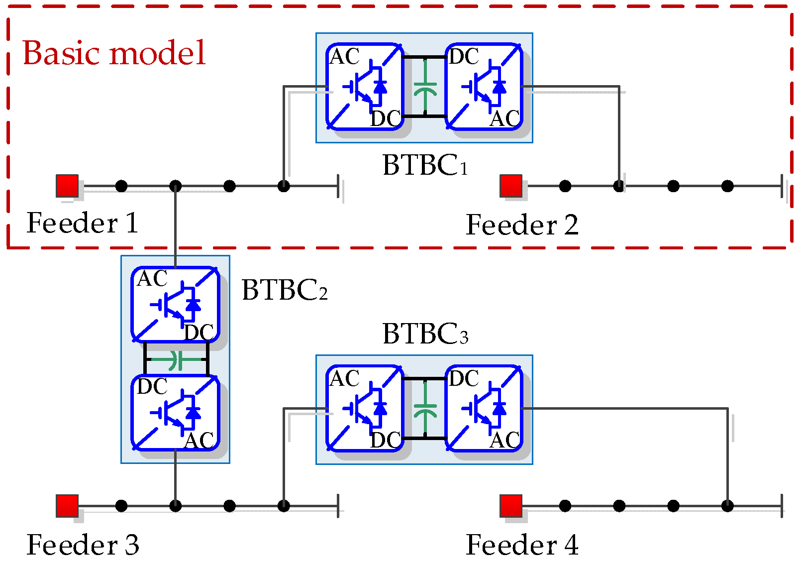
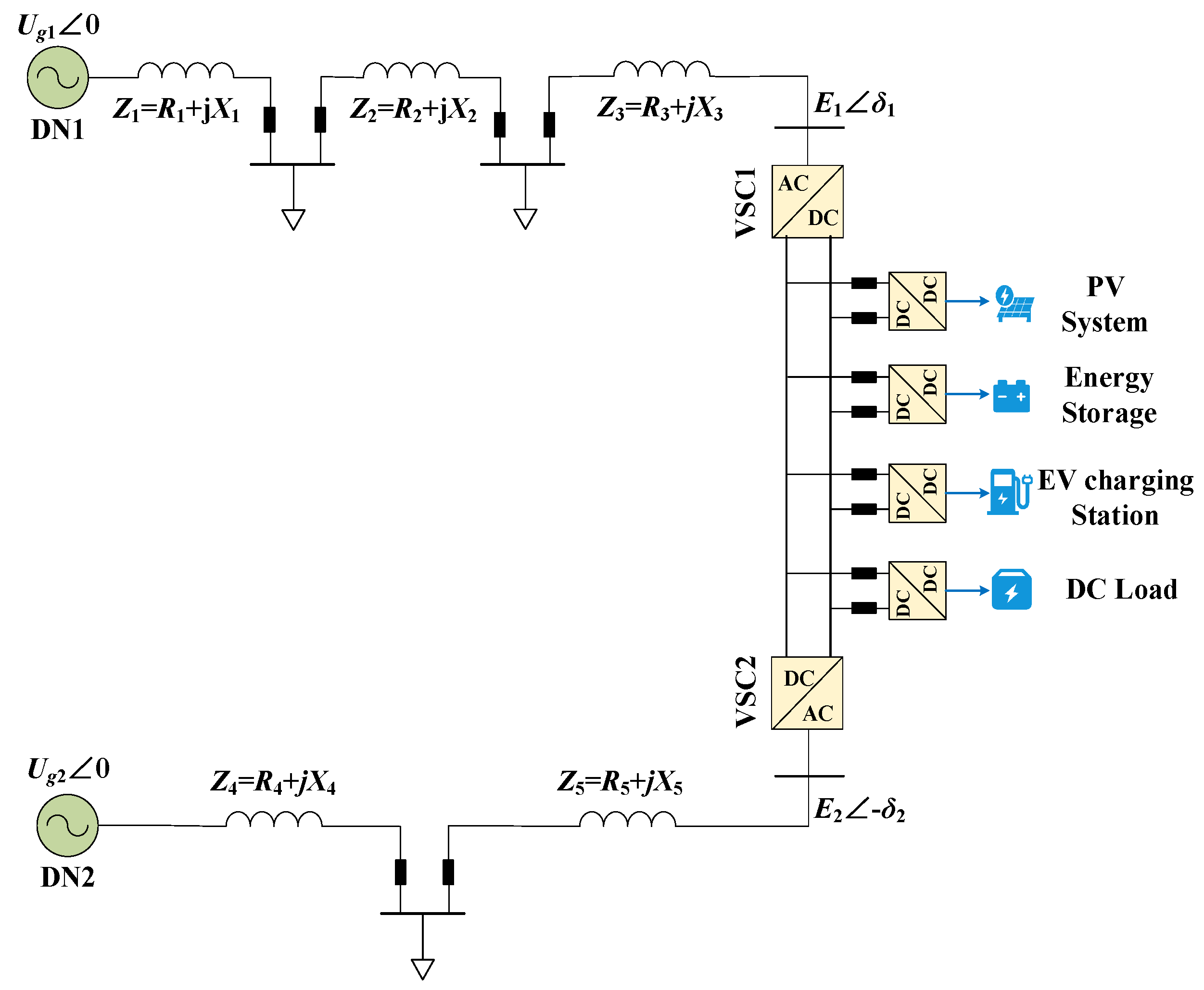
The general structure of a BTBC-FMSS-based flexible interconnected DN is shown in Figure 1, which is composed of multiple feeders and multiple interconnected BTBC-FMSS devices. It is worth pointing out that the diversity of the FMSS topology leads to the diversity of flexible interconnected DNs. Generally, FMSS can be divided into a variety of types, such as double-terminal interconnection [16], multi-terminal interconnection [17], cross-voltage level interconnection and AC-DC hybrid interconnection [18]. Among them, the two-AC-DN system adopts the two-terminal interconnection (BTBC-FMSS) networking mode as its basic type. In this interconnection mode, the two ends of the distribution network can not only isolate each other and operate independently, but also dynamically adjust the interactive power when necessary, balance the load rate level of the feeders of the two sides of the DN, provide the contact channel at the same time, and effectively block the fault current propagation. Therefore, this paper takes the DN system of BTBC-FMSS interconnection as the research object.
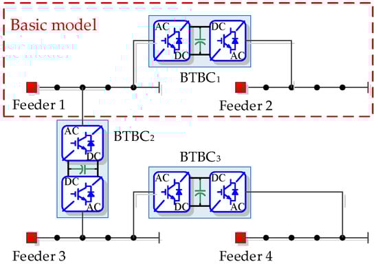
Figure 1.
The structure diagram of the BTBC-FMSS-based flexible interconnected DN system.
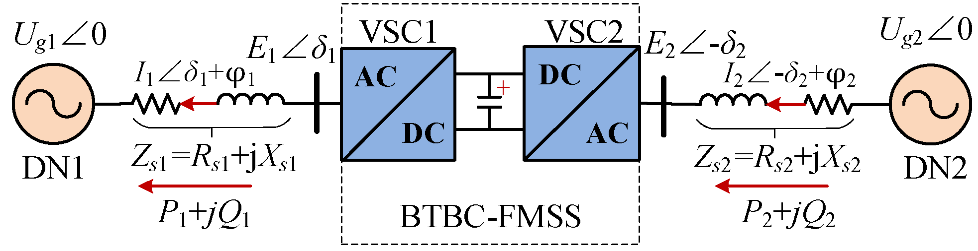
In this paper, the transmission power limit of basic flexible interconnected DNs (two distribution networks connected by a single BTBC-FMSS) is studied. Firstly, the DN system on both sides is equivalent simplified to form a double-ended power supply system, as shown in Figure 2. After a series of star triangle transformations, the load and line are equivalent to the two impedance Zs1 and Zs2 of the AC-DN system, and the voltage sources at both ends are represented by Ug1 and Ug2. Zs1 is the equivalent impedance between the converter VSC1 side and AC system 1 (DN1), which is composed of line impedance Zline, load Zload on PCC and equivalent impedance Zg1 of AC system 1. After star triangle transformation, it is expressed as Zs1 = rs1 + jxs1 = |Zs1|∠θz1. Similarly, Zs2 is the equivalent impedance between the terminal side of the converter VSC2 and the AC system 2 (DN2), expressed as Zs2 = rs2 + jxs2 = |Zs2|∠θz2. E1 and E2 indicate the side voltage amplitude of converter VSC1 and VSC2, respectively.

Figure 2.
The Equivalent circuit of the BTBC-FMSS-based flexible interconnected DN system.
In addition, to further facilitate the analysis of the problem, the VSC1 terminal side is set to adopt the inverter convention, and the output current is positive. The VSC2 side adopts the rectifier convention, which considers the input current to be positive. Therefore, δ1 is the phase difference of VSC1 side voltage E1 ahead of the grid voltage Ug1. δ2 is the phase difference of the grid voltage Ug2 ahead of the VSC2 side E2. δ1 and δ2 can also be considered as the power angles of the VSC on both sides.
2.2. Control Strategy Analysis of Flexible Multi-State Switch
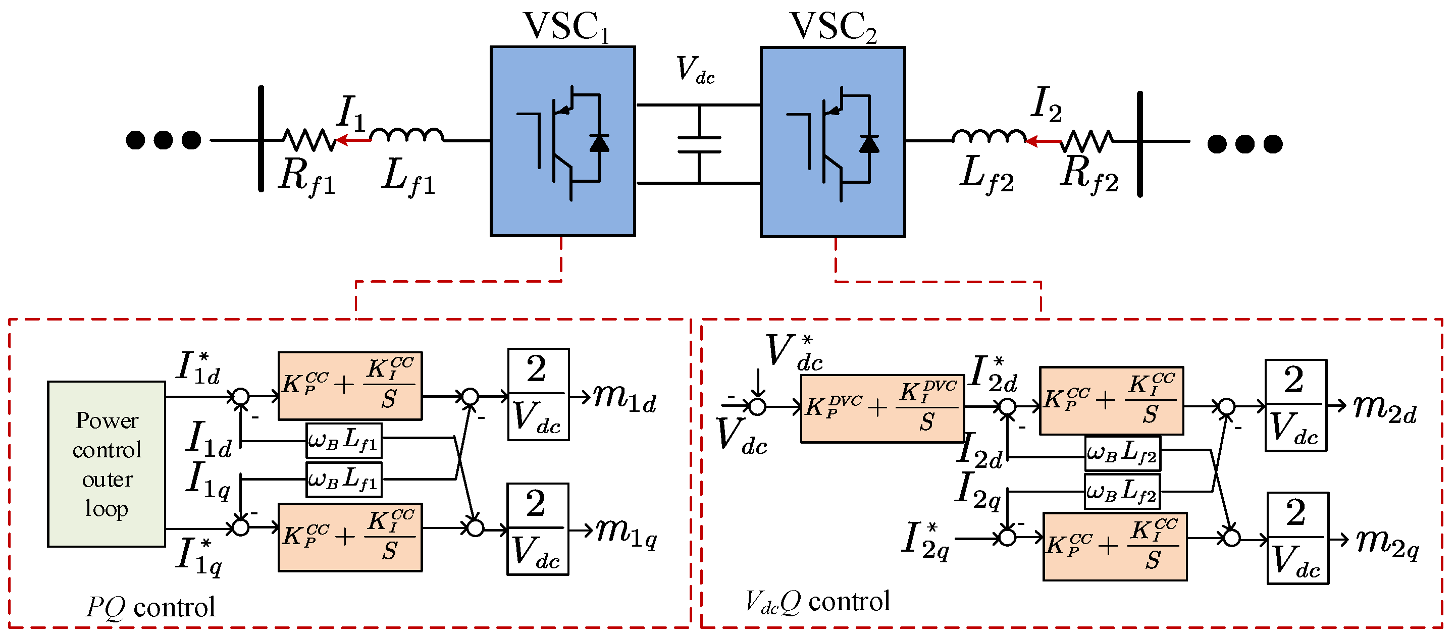
The detailed control architecture of VSC on both sides of BTBC-FMSS is shown in Figure 3. In normal operation, one end of the BTBC-FMSS uses power control strategy (PQ control), while the other end uses DC voltage control strategy (VdcQ control). Since the positive direction of transmission power for the BTBC-FMSS determined in this paper is set as VSC2→VSC1, PQ control is adopted for the VSC1 side and VdcQ control is adopted for the VSC2 side to facilitate the analysis of the problem. It is worth pointing out that the setting of the positive direction and the control mode on both sides does not affect the analysis result of the final power transmission relationship.
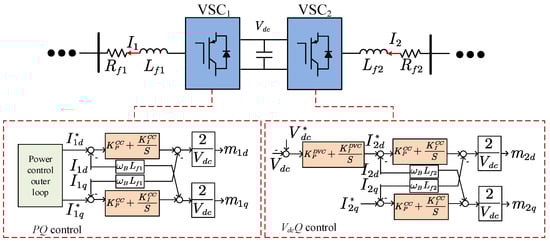
Figure 3.
The control block diagram of BTBC-FMSS device.
Both sides of BTBC-FMSS VSC adopt the current control mode; so, the inner loop of the controller only contains the current loop, which is expressed as follows [19,20]:
where and are the dq axis voltage reference values of VSCs on both sides; , and , are, respectively, measured and reference values of the dq axis current of VSCs on both sides; and are the PI control parameters of the current inner loop; and i = 1, 2.
The external loop of VSC1 uses PQ control to determine the active and reactive power output where the references are decided from the upper-level dispatching command or the local power grid status. The power loop is to make the difference between the reference value of the power and the actual value, and then through the PI control, to realize the error-free control of the power reference, as shown in Formula (2).
where , and , are the measured and reference values of the output active and reactive power of VSC1, respectively. and are the PI control parameters of the power outer loop.
The VSC2 side is controlled by VdcQ to maintain the voltage stability of the capacitor on the DC side of the BTBC-FMSS, and then realize the power balance of the two sides of the VSC. The corresponding controller expression is as follows:
where E2d is the d-axis measured value of the output voltage on the VSC2 side. is the reference value of the output reactive power of the VSC2 side. Vdc and
are the measured values and reference values of the DC voltage of BTBC-FMSS
and
are the PI control parameters of the outer loop of the DC voltage.
3. Derivation of Transmission Power Expression of Flexible Multi-State Switch
According to the analysis in Section 1, current control modes are generally adopted at both ends of BTBC-FMSS under a quasi-steady state. Therefore, the transmission power limit analysis method given in the literature [9,10] based on the circuit correlation between the distribution network voltage and inverter terminal voltage is not accurate. In this section, the transmission power expressions on both sides of BTBC-FMSS are derived in detail according to the current source control circuit expression.
3.1. The Transmission Power Expression of VSC Controlled by Current under dq Transformation
Firstly, according to the Park transformation principle, the expression of the transmission power on both sides of VSC1 and VSC2 in the dq coordinate system is written, as shown in Equation (4).
where Pi and Qi denote the active and reactive power output from the VSCi side, respectively; Eid and Eiq denote the voltage components in the d and q axes of the VSCi side, respectively; and Iid and Iiq denote the current components in the d and q axes of the VSCi side, respectively.
In addition, converters generally adopt d-axis voltage orientation, that is, Eiq = 0; so, Equation (4) can be further written as follows:
Due to the d-axis voltage orientation, Pi and Qi are approximately proportional to Iid and −Iiq when Eid does not change much, the approximate decoupling of active and reactive power control is realized, and the constant current control can be converted into constant power control. It is worth pointing out that Equation (5) cannot directly reflect the functional relationship between the output power Pi + jQi on the VSCi side and its output current Ii and power angle δi, which needs to be further derived according to the vector diagram.
3.2. Derivation of Transmission Power Expression of VSC on Both Sides of BTBC-FMSS
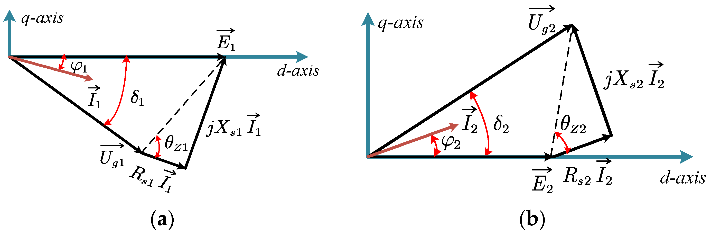
Firstly, the vector relationship of voltage and current between VSCi and distribution network on both sides in the dq coordinate system is drawn, as shown in Figure 4a,b.
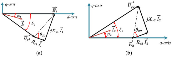
Figure 4.
Vector diagram of BTBC-FMSS both sides: (a) VSC1 side vector relationship; (b) VSC2 side vector relationship.
As can be seen from Figure 4a, since VSC1 adopts the inverter tradition, the VSC1 terminal voltage E1 is ahead of the power grid voltage Ug1. Based on the vector relationship, the expression of E1 in d and q axis components can be derived as follows:
where δ1 denotes the phase difference between the machine terminal voltage E1 on the VSC1 side and the grid voltage Ug1, I1 denotes the current amplitude on the VSC1 side, |Zs1| denotes the amplitude of the equivalent impedance on the VSC1 side, θz1 denotes the phase angle of the equivalent impedance on the VSC1 side, and φ1 denotes the power factor angle on the VSC1 side.
By substituting E1d in the above equation into Equation (5), the transmission power expression of VSC1 side under d-axis voltage orientation can be written as follows:
Similarly, by adopting the rectifier tradition on the VSC2 side, the expression of E2 in the d and q axes’ components can be obtained:
where δ2 denotes the phase difference between the machine terminal voltage E2 on the VSC2 side and the grid voltage Ug2, I2 denotes the current amplitude on the VSC2 side, |Zs2| denotes the amplitude of the equivalent impedance on the VSC2 side, θz2 denotes the phase angle of the equivalent impedance on the VSC2 side, and φ2 denotes the power factor angle on the VSC2 side.
Similarly, by substituting E2d into Equation (5), the transmission power expression of VSC2 side under d-axis voltage orientation can be written:
The expressions of active and reactive power transmission power shown in Equations (7) and (9) are related to the two controlled variables of output current amplitude Ii and power factor angle φi at the VSCi side, but there is still the uncontrolled variable power angle δi to be further replaced.
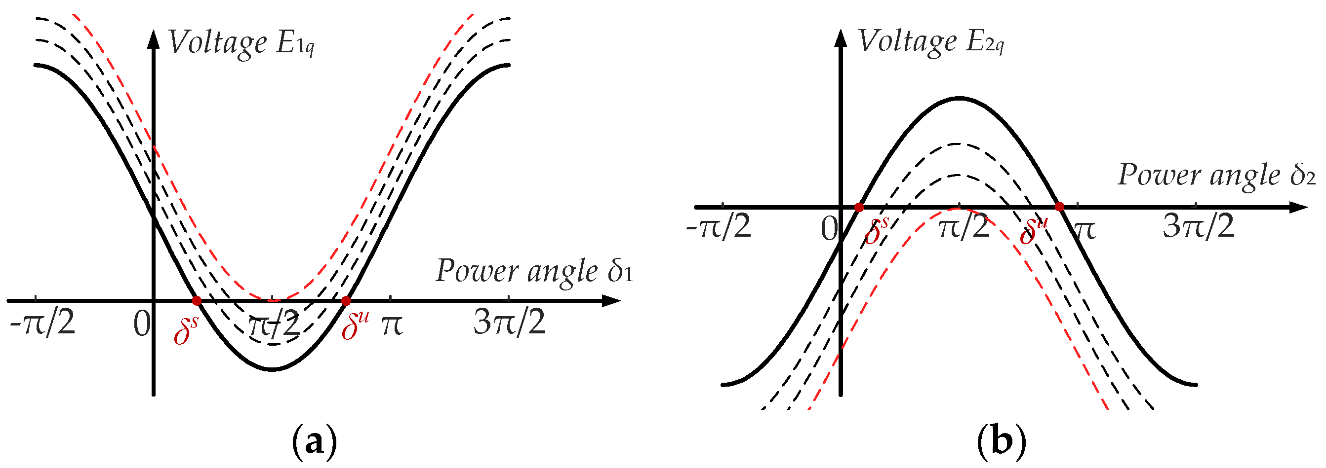
Considering that the VSC on both sides adopts the d-axis voltage orientation and the PLL adopts the q-axis voltage Eiq phase locking, the Eiq = 0 element is valid under the steady-state condition of the system, and the relationships between E1q and δ1 and E2q and δ2 are plotted, respectively, as shown in Figure 5a,b.
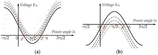
Figure 5.
q axis voltage and power angle relationship of VSCi: (a) relationship between VSC1 side voltage and power angle; (b) relationship between VSC2 side voltage and power angle.
In the above figure, there are two operating points for the δi angle of VSC on both sides under the condition that Eiq = 0 is met. According to the small-signal stability analysis, the static stable operating point of δi can be determined, as shown in Equation (10).
Obviously, according to the solution constraint, the condition ≤ π/2 is obtained.
By substituting the result of the above stable operating point into Equations (7) and (9), the transmission power expressions of VSC on both sides can be further written as follows:
- (1)
- VSC1 side,
- (2)
- VSC2 side,
It can be seen from Expressions (11)–(14) that when the VSC on both sides adopts the current control mode, its output power expression contains only two controlled variables: the output current amplitude Ii on both sides and the power factor angle φi, which is the transmission current vector . It can also be seen from the analysis of Equations (11) and (14) that the active and reactive transmission power are also related to the two structural parameters of the power network intensity Ugi/|Zsi| and the equivalent impedance angle of the power network φi.
In addition, the observation Formulas (11)–(14) show that the expressions of active and reactive power show some symmetry in form, that is, there is translation and axial symmetry in the active and reactive power characteristics of VSCi, which is expressed as follows:
Through symmetry analysis, we can know that only the active power transmission characteristics are given, and then the reactive power transmission characteristics can be obtained by translation and axisymmetric transformation. Therefore, if not specified below, only the corresponding analysis of the output active power characteristics of the VSCi on both sides of the BTBC-FMSS is carried out.
4. Transmission Power Limit and Stable Operation Domain Analysis of BTBC-FMSS
Section 3 derives the expression of the transmission power of the VSC on both sides of the BTBC-FMSS under the current control. This section will further analyze the transmission power limit and stable operation domain of the BTBC-FMSS equipment according to the table, and discuss its relationship with the BTBC-FMSS stability.
4.1. Analysis of Transmission Power Characteristics on Both Sides of BTBC-FMSS
BTBC-FMSS has the ability of four-quadrant operation, and there is also a potential demand for four-quadrant operation in DN. Therefore, if the output current amplitude Ii and power factor angle φi of the VSC on both sides are in the range of Ii ≥ 0, φi∈[−π, π]. Then, the output active and reactive power of VSC on both sides should be regarded as binary functions with respect to the above two variables, expressed as Pi(Ii, φi) and Qi(Ii, φi), i = 1, 2.
Under the constraint of the existence of static stable working point of PLL, the input variable of PLLi integrator of VSCi on both sides of BTBC-FMSS must be strictly 0, that is, Eiq = 0. If the special angle αi is further defined as the sum of the impedance angle θzi and the power factor angle φi, that is, αi= θzi + φi, then using Eiq = 0 and according to the Formulas (5) and (10), the value range of Ii can be calculated, expressed as follows:
What really affects the power transmission direction should be the power factor angle φ. When the range of the power factor angle is [−π/2, π/2], the direction of power transmission is forward, i.e., from VSC2 to VSC1; when the range of the power factor angle is [π/2, 3π/2], the direction of power transmission is inverted, i.e., from VSC1 to VSC2. Therefore, it is clear that the transmission direction has nothing to do with the impedance angle θz.
However, in this paper, in order to facilitate the analysis, we defined the special angle α to be the sum of power factor angle and impedance angle, that is α = θz + φ, which does not change the fact that the transmission direction is only related to the power factor Angle φ.
Considering the four-quadrant operation capability of VSCi, there is Ii ≥ 0, φi∈[−π, π], and the equivalent impedance angle of the power grid on both sides θzi∈[0, π/2], i = 1, 2. Thus, θzi + φi∈[−π + θzi, π + θzi]. Under different values θzi + φi, the upper limit Iimax of Ii exists as follows:
As can be seen from the above formula, when θzi + φi = 0 and θzi + φi = π (that is, φi and θzi are opposite or complementary to each other), the output/input current on the VSCi side has no upper limit, and is only influenced by the capacity of the VSC itself.
In addition to the inherent limit of VSCi input/output current, it is known from Equations (11)–(14) that there is a complex non-linear relationship between VSCi input/output power and input/output current and power factor angle. At the same time, because of the symmetry of Equations (11)–(14), this paper mainly focuses on the active power transmission capability of BTBC-FMSS. Therefore, taking the VSC1 side of Equation (11) as an example, the expression of transmission power limit is derived.
Firstly, according to Formula (11), using the condition of dP1/dI1 = 0, the critical current of P1 with extreme value is obtained, which is expressed as follows:
According to the above formula, in the special case of α1 = 0, the critical current tends to infinity because there is no constraint on the output current. By replacing Formula (18) with the Formula (11), the extreme value P1cr of the transmitted active power on the VSC1 side can be obtained, which is expressed as follows:
In the above formula, K1cr(α1) is a coefficient only related to the special angle α1. In the quasi-steady state, Sac1 is approximately the short-circuit capacity sent by the distribution network 1 to the VSC1 side. K1cr (α1) and Sac1 can be further expressed as follows:
According to the above formula, the magnitude of the extreme P1cr of the transmitted active power on the VSCi side is only related to the short-circuit capacity Sac1 and the special angle α1 on the grid side, and the transmission direction is only determined by the power factor angle φ1 = α1 − θZ1.
Formulas (18)–(20) give the expression of the transmission active power extreme value P1cr and the corresponding critical current I1cr on the BTBC-FMSS VSC1 side. According to the maximum function theorem, the maximum value of a continuous function can only be obtained at the end of the interval or the extreme point. For VSC1 side, according to Formula (17), the variation norm of the output current I1 is [0, I1max]; so. if (17) is substituted into (11), the expression of P1 (I1max) can be deduced as follows:
In the above formula, K1m(α1) can be expressed as follows:
Similarly, the critical current I2cr of the transmitted active power P2 on the VSC2 side can be obtained, which is expressed as follows:
Correspondingly, the transmission active power extreme value P2cr on the VSC2 side is expressed as follows:
In the above formula, K2cr(α2) and Sac2 can be expressed as follows:
Similarly, by substituting (17) into (13), the expression of P2 (I2max) can be deduced as follows:
In the above formula, K2m(α2) can be expressed as follows:
Obviously, the comprehensive Formulas (18)–(27) show that the limit of the transmission power of the VSC on both sides of the BTBC-FMSS is mainly determined by the extreme value Picr on each side and the interval endpoint values Pi(Iimax) and Pi(0). In addition, it is obvious that the expressions of Picr and Pi (Iimax) are only related to the power factor angle φi(αi) of the controlled variable. Therefore, if the curves of Picr − αi, Pi(Iimax) − αi and Pi = 0 are drawn, the closed area surrounded by each curve is the static stable operation domain on each side for the VSCi. The static stable operation domain of each side of BTBC-FMSS is intuitively analyzed with a specific example.
Table 1 shows the typical specific values of the equivalent circuit of the BTBC-FMSS flexible interconnection DN as shown in Figure 2. Among them, to control the control variables to facilitate the problem analysis, it is assumed that the physical and control parameters of the VSC on both sides of the BTBC-FMSS are the same, and the equivalent impedance parameters and voltage levels of the flexible interconnected DN on both sides of the BTBC-FMSS are completely the same. In addition, the corresponding stable operation domains of the VSC on both sides are given.

Table 1.
The structure and control parameters of flexible interconnected distribution network.
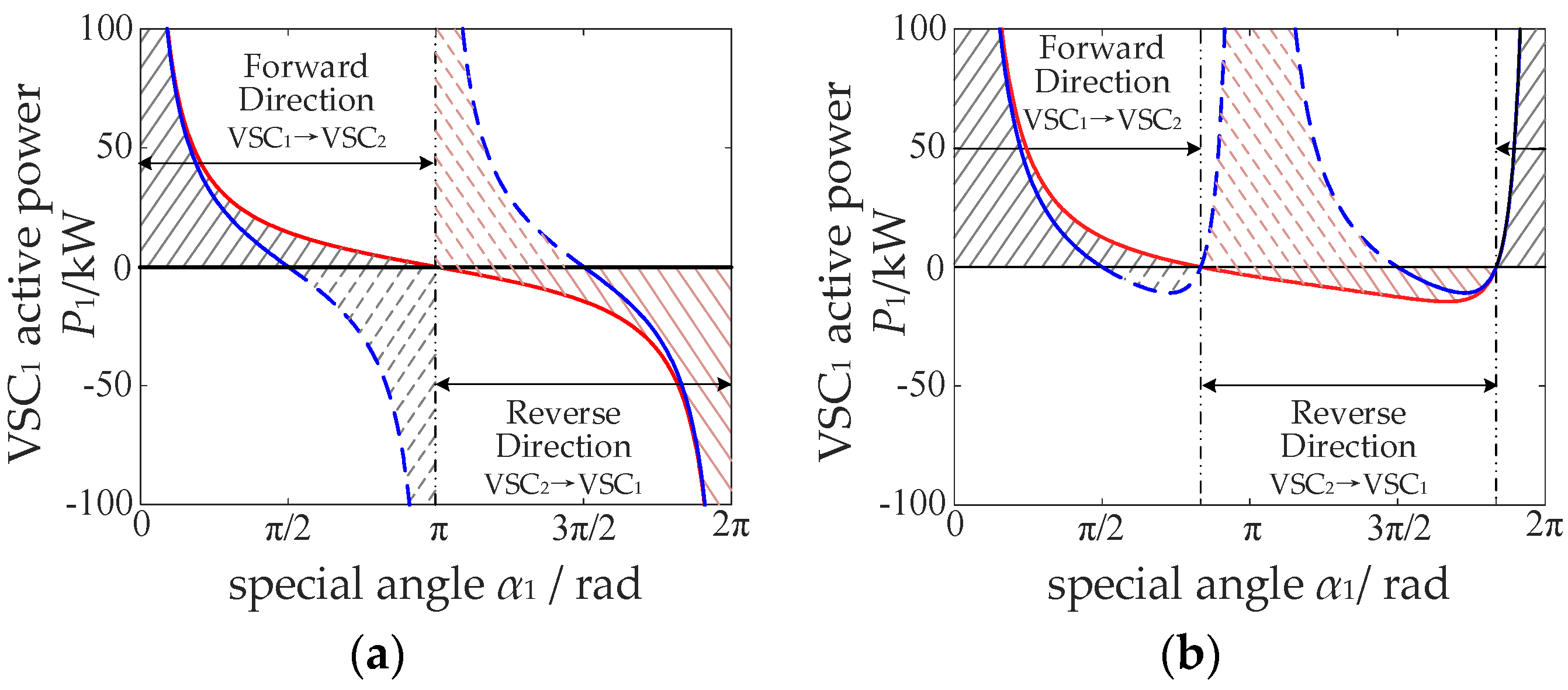
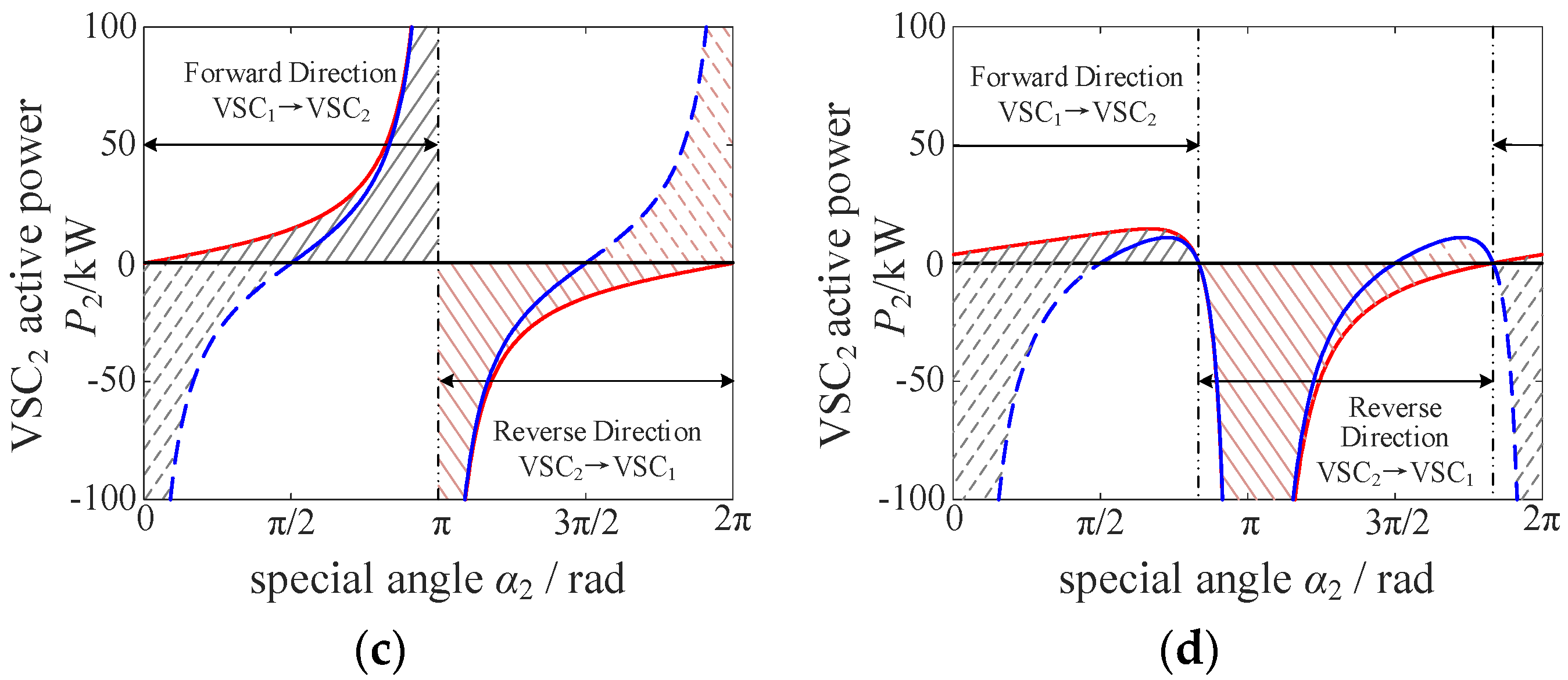
The static stable operation domain of the VSC on both sides of the BTBC-FMSS at different impedance angles is shown in Figure 6. Figure 6a,b corresponds to two cases of VSC1 side θZ1 = π/2 and θZ1 = π/3, respectively, and Figure 6c,d corresponds to two cases of VSC2 side θZ2 = π/2 and θZ2 = π/3, respectively. The red line represents the Picr − αi curve, the blue line represents the Pi(Iimax) − αi curve, and the black line represents the Pi = 0 curve. The gray shaded area represents the stable operation domain of active power forward transmission, which is expressed as SD1, and the light red shadow represents the stable operation domain of active power reverse transmission, which is represented as SD2. In addition, the realization indicates that the output current direction of the VSCi side is the same as the active power direction, and the dotted line indicates that the two directions are opposite.
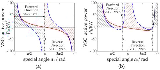
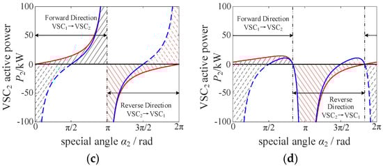
Figure 6.
The static stable operation region of BTBC-FMSS for two-sided VSCs active power transmission, (a) θz1 = π/2, P1 − α1 curve; (b) θz1 = π/3, P1 − α1 curve; (c) θz1 = π/2, P2 − α2 curve; (d) θz1 = π/3, P2 − α2 curve.
Looking carefully at Figure 6a–d, the following conclusions can be drawn by comparison:
(1) The Picr curve takes 2π as the period, and the Pi (Iimax) curve takes π as the period, and the static stable operation domain surrounded by them and Pi (0) is unbounded when the conditions of αi = 0 and αi = π are satisfied.
(2) When the line impedance is approximately pure inductance (θzi = π/2), with αi = π as the boundary, the static stable operation domain of each side of VSC with forward and reverse transmission is the same and the center is symmetrical, that is, the stable operation domain is the same in different transmission directions.
(3) In the inductive line (θzi = π/3), there is a difference in the stable operation domain of the forward and backward transmission power of each side of the VSC, that is, the feasible region of stable operation in different directions is different.
(4) Under the same impedance angle and short-circuit capacity, the static stable operation domain of forward transmission on the VSC2 side is symmetrical with the static stable operation domain of the reverse transmission on the VSC1 side, and vice versa.
(5) The static stable operation domain (solid line + dashed line region) under the current control mode is larger than that under the power control mode (solid line region). The reason is that the current control is stored in the operation point where the VSC current is negatively related to active power and can operate normally.
4.2. Stable Operation Domain Analysis of BTBC-FMSS
First, it is important to point out that the active and reactive power transmission characteristics of the BTBC-FMSS are fundamentally different: (1) For the active power transmission problem, since the BTBC-FMSS is equivalent to an active transmission channel, the equation P1 = P2 necessarily exists in the steady state while ignoring the power loss on the DC side. (2) For the reactive power transmission problem, due to the complete decoupling of the reactive power control on both sides, the BTBC-FMSS should be regarded as a bi-directional reactive power supply, and the size and direction of Q1 and Q2 are not necessarily related to each other but only to the reactive power control mode.
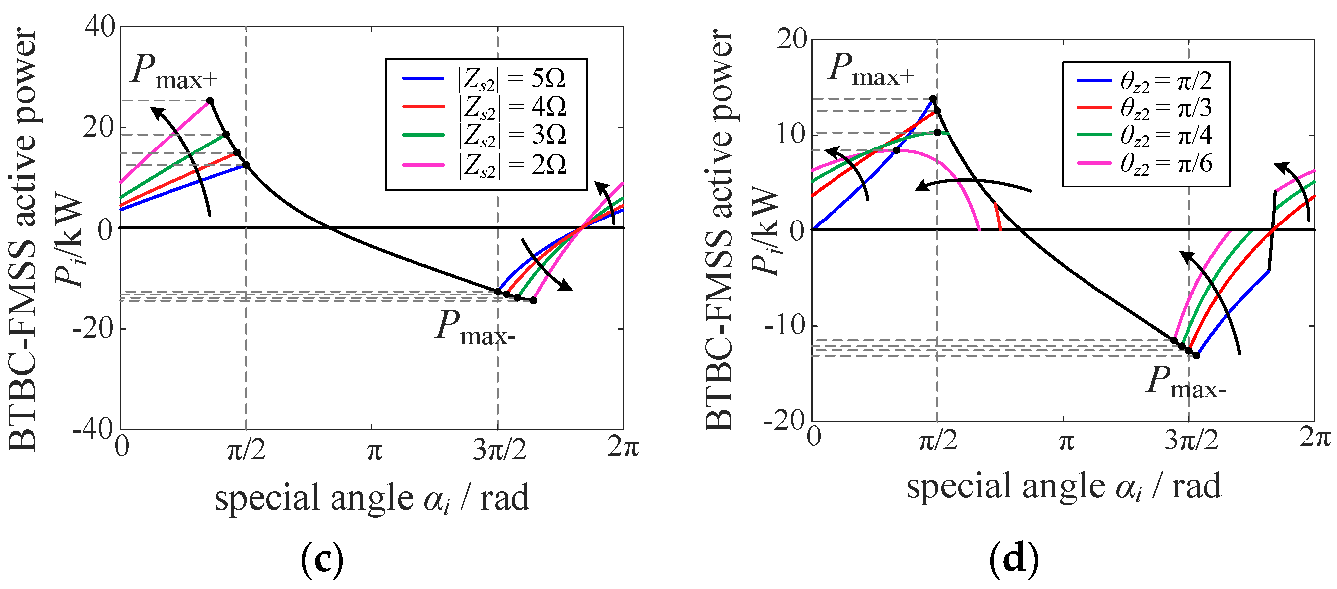
Secondly, it is considered that in a real flexible interconnected DN system, at the steady state, balancing the load ratio of feeders on both sides as an active transmission channel is the BTBC-FMSS’s core mode of operation. On the one hand, affected by the capacity, the proportion of reactive power transmission is too large to crowd the active transmission channel, and the reactive power transmission should be used as an auxiliary function without or with less transmission; on the other hand, the reactive power balancing in the grid should try to follow the principle of in situ, and a larger reactive power transmission will undoubtedly increase the active loss of the device. In addition, most studies also believe that even if the BTBC-FMSS can transmit reactive power, the reactive power control on both sides of it should establish a correlation relationship. Therefore, this paper further selects a special transmission mode, i.e., equal-capacity transmission mode (). Obviously, in the equal capacity transmission mode, the intersection of the static stabilized operating areas of the VSCs on both sides is the static stabilized operating area of the whole device of the BTBC-FMSS. Considering the actual operation scenario, the equivalent impedance of each side of the BTBC-FMSS cannot be simply regarded as pure inductance, and the values and impedance angles of the equivalent impedance may be different, but the voltage levels of the feeder lines on both sides of the DN are generally the same. Therefore, to facilitate the analysis, the parameters of fixed DN1 remain unchanged, two scenarios of θZ1 = π/2 and θZ1 = π/3 are selected to change the short-circuit capacity (equivalent impedance module value|Zs2|) and impedance angle θz2 of DN2, respectively, and the static stable operation domain of BTBC-FMSS as shown in Figure 7a–d is obtained.
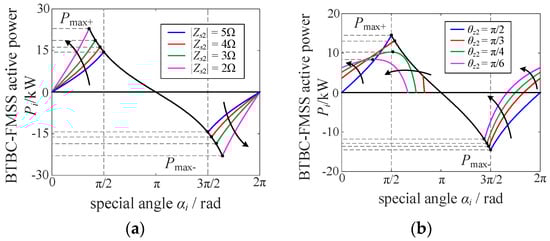
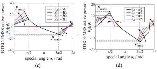
Figure 7.
The static stable operation domain of BTBC-FMSS for active power transmission, (a) θz1 = π/2 with |Zs2|variations, (b) θz1 = π/2 with θz2 variations; (c) θz1 = π/3 with |Zs2| variations; (d) θz1 = π/3 with θz2 variations.
As shown in Figure 7, the black solid line represents the P1cr curve, and different colored solid lines represent the gradient of the P2cr curve. The irregular closed area surrounded by P1cr, P2cr and Pi = 0 is the static stable operation domain of the BTBC-FMSS device, which is expressed as SD = SD1∩SD2. A careful analysis of the above two pictures shows that the following conclusions can be drawn:
(1) Different from the separate analysis of VSC static stable operation domain on each side, the static stable operation domain of BTBC-FMSS must be bounded under forward/reverse transmission, and there is a maximum upper limit of transmission active power, which is Pmax+ in forward transmission and Pmax− in reverse transmission.
(2) If the short-circuit capability and impedance angle of the DN on both sides are the same, that is, Ug1 = Ug2, |Zs1| = |Zs2|, when θZ1 = θZ2, the maximum transmission power limit of BTBC-FMSS forward and reverse must be obtained at π/2 and 3 π/2, and SD+ = SD−.
(3) With the increase in the short-circuit capability of the VSC2 side (in Figure 7a), the overall transmission power limit of the BTBC-FMSS increases significantly, and the SD area expands significantly.
(4) When the equivalent circuit impedance angle of the VSC2 side is reduced (in Figure 7b), the overall transmission power limit of the BTBC-FMSS is reduced, the SD decreases slightly under the forward transmission, and the SD decreases obviously under the reverse transmission.
According to conclusion 1, the maximum active power transmission limits of BTBC-FMSS in forward and reverse transmission directions are Pmax+ and Pmax−, respectively, and can be obtained by solving the intersection of P1cr and P2cr. However, when the parameters of the distribution network on both sides of the BTBC-FMSS are asymmetric, the analytical expression is difficult to obtain, and it can only be obtained by depicting the stable operation domain in practical application.
4.3. Transmission Active Power Limits Analysis and Enhancement Measures of BTBC-FMSS
(1) The analysis of BTBC-FMSS in the previous section shows that there must be a stability limit of transmission power in BTBC-FMSS in different transmission directions, and the limit is only related to the short-circuit capacity, line impedance angle and power factor angle of the power grid on both sides. The corresponding calculation flow chart can be shown as Algorithm 1:
| Algorithm 1: BTBC-FMSS transmission power stability limit algorithm. |
| 1: The Thevenin equivalent of the BTBC-FMSS based flexible interconnected DN on both sides is carried out. |
| 2: Get the equivalent impedance on both sides: |
| 3: Zs1 = |Zs1| ∠ θ1 |
| 4: Zs2 = |Zs2| ∠ θ2 |
| 5: Calculate, derive the maximum input/output current amplitude I1max and I2max. |
| 6: Make drawings, derive the stable operation domain SD1 and SD2. |
| 7: Take the intersection, SD = SD1∩SD2 (Figure 6) |
| 8: Derive Pmax+ and Pmax− (the maximum upper limit of active power transmission). |
| end |
(2) Enhancement measures to improve static stability
Measure 1: The VSC sides on both sides use the local reactive power compensation devices (capacitors) as the parallel reactive power compensator.
The advantage of local reactive power compensation is that it can support the voltage of VSC sides on both sides, improve the short-circuit capacity of AC system to a certain extent, and leave enough active power transmission channels.
Measure 2: The transmission of active and reactive power distribution ratio is adjusted according to the actual situation (adjust the power factor angle φi).
It can be seen from Figure 7 that the pure active power transmission mode often does not correspond to the maximum transmission active power limit, because the equivalent impedance angle of the DN on both sides is not strictly equal to π/2. In the absence of a local reactive power compensation device, properly adjusting the distribution ratio of active and reactive power is helpful to improve the transmission capacity of active power.
(3) Potential challenges and future research directions
Firstly, the potential challenges of the method proposed in this paper lie in the acquisition of grid equivalent impedance, which may be difficult to calculate when there are many nonlinear loads and distributed generators in the distribution network.
Secondly, this paper only investigates the BTBC-FMSS in conventional control scheme (PQ control for VSC1 and VdcQ control for VSC2). However, in some cases, such as in fault condition, one of the VSC side can transfer into the virtual synchronous generator (VSG) control scheme. Thus, further discussion and research of its stable operation domain are needed.
Finally, in a multi-terminal (more than two VSC terminals) LVDC system, the constraints on power transmission for FMSS device can be presented as Pvsc1 + P vsc2 + …+P vscn = 0. Therefore, how to visualize the stable operating domain of FMSS device in this case is also one of the future research directions.
4.4. The Engineering Application Prospect of the Stable Operation Domain of BTBC-FMSS and the Specific Suggestions for the Actual Distribution Network
The flexible multi-state switching stable operation domain proposed in this paper can be applied to two typical scenarios: one is the BTBC-based interconnected microgrid clusters, and the other is the low-voltage direct current (LVDC) system.
Scenario I: Interconnecting multiple microgrids (MGs) to form a larger-scale interconnected MGs (IMGs) is an ideal way to increase the penetration rate of distributed generation (DG) and improve the reliability of power supply for the whole system. In addition to the conventional impedance lines interconnection scheme, nowadays, a new interlinking way, by using back-to-back converters (BTBCs), has become a novel interconnection scheme to solve the integration problems of IMGs. Usually, MG can be viewed as a weak grid since there is only a limited power supply and a weak grid structure. In such a system, the BTBC device is likely to have the transmission limit due to the constraint of stable operation domain.
Scenario II: More and more distributed energy sources, such as photovoltaic systems and wind power, are connected to the power grid through DC-DC or AC-DC converters, which, coupled with the wide application of DC devices such as electric vehicles, LEDs, and energy storage, has promoted the rapid development of low-voltage DC systems and AC-DC hybrid systems. In such a DN system, at the end of the feeders, the analysis of stable operation domain for the BTBC is necessary.
The specific suggestions for the actual distribution network about implementing BTBC-FMSS stable operation domain can be summarized in the following two points:
(1) The stable operation domain is both influenced by the short-circuit capacity and controller design on both sides of BTBC. Basically, the weaker the system, the more important it is to discuss the stable operating domain of BTBC. The two typical application scenarios are presented above.
(2) For a given capacity BTBC-FMSS device in DN, the main task is to evaluate its stable operation domain in real time comparing with its capacity. The intersection of the two is the actual stable operation domain for the BTBC-FMSS. In other words, the initial capacity planning for BTBC-FMSS should also refer to the verification of the stable operation domain, and the two issues are interactively coupled.
5. Simulation Results
To verify the validity of the proposed analysis method for BTBC-FMSS power transmission limit and static stability, the simulation verification model shown in Figure 8 is built in Matlab/Simulink. The structural and control parameters of distribution network and BTBC-FMSS devices are shown in Table 2, and the impedance parameters of distribution lines and loads on both sides are shown in Table 3.
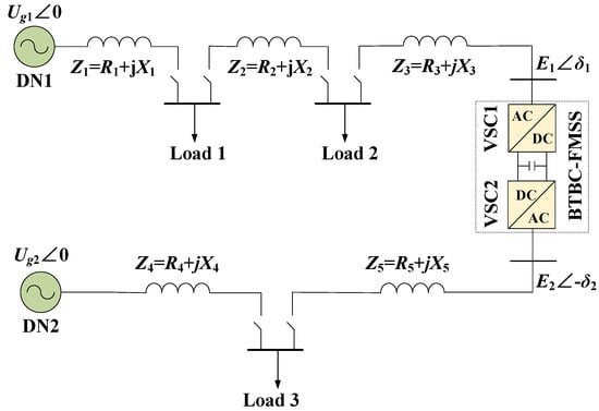
Figure 8.
The simulation circuit of the BTBC-FMSS-based flexible interconnected DN system.
Table 2.
The structure and control parameters of flexible interconnected DN.
Table 3.
Structural parameters of flexible interconnected distribution grids before and after Davening equivalence.
According to Thevenin’s equivalent method, the equivalent impedance parameters of the DN system on both sides under full load access are Zs1 = 4.55 Ω, Zs2 = 9.85 Ω, Ug1 = 324, Ug2 = 361.1, and equivalent voltage.
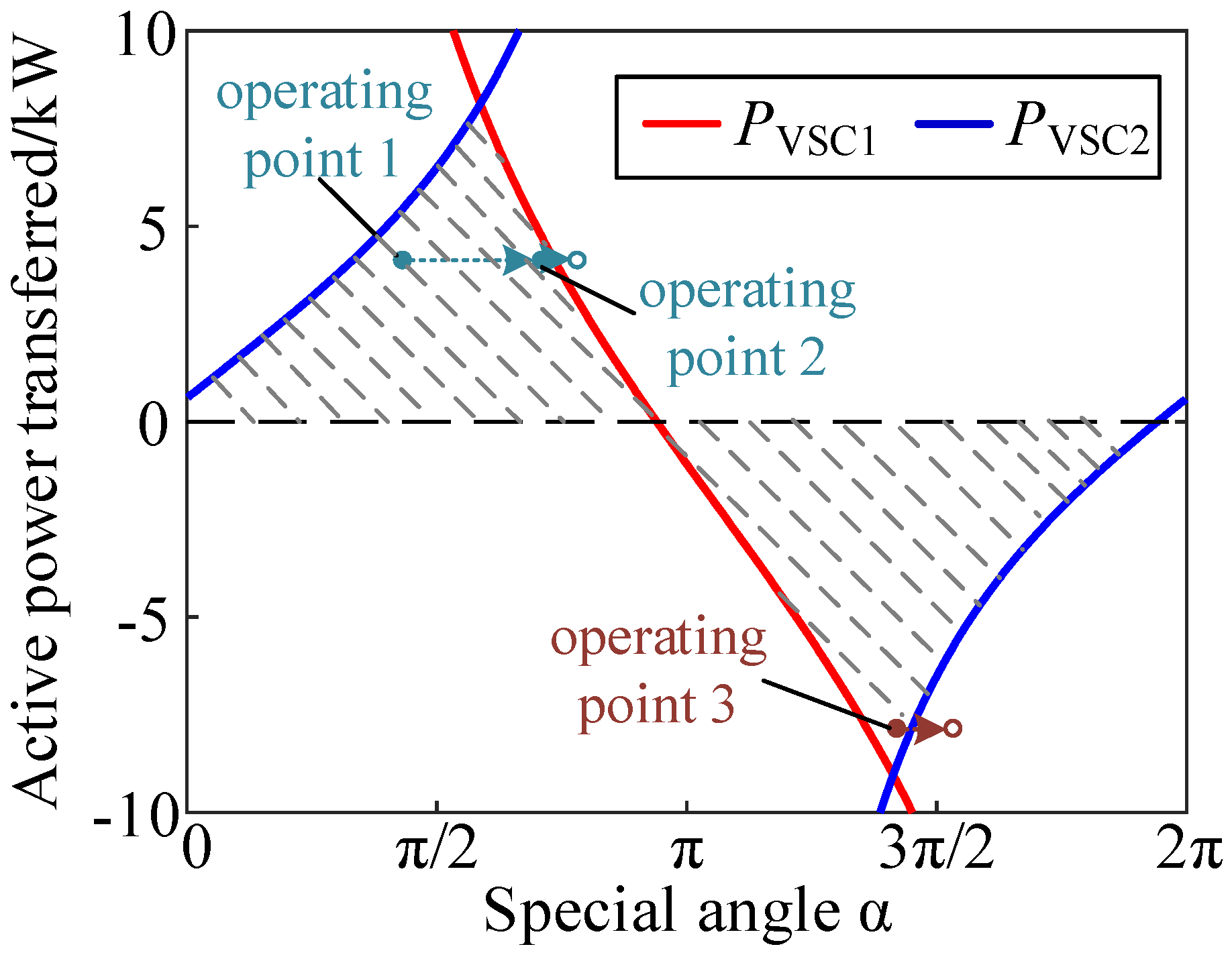
According to the derivation process of this paper, the stable operation domain of BTBC-FMSS can be made under the simulation example, as shown in Figure 9.
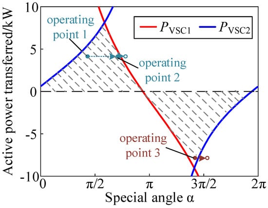
Figure 9.
Stable operation domain of BTBC-FMSS under simulation cases.
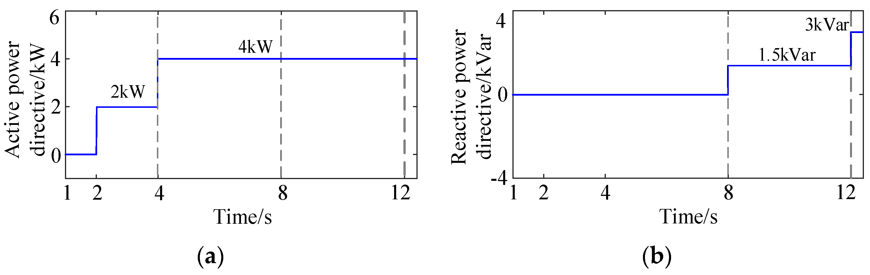
Case 1: All loads are connected to the system at the beginning of the simulation, and the active and reactive power transmission references are set to 0. For active power control, the active power transmission references are changed into 2 kW and 4 kW at 2 s and 4 s, respectively; for reactive power control, the reactive power transmission references on both sides of VSC are changed into 1.5 kVar at 8 s time, and the simulation ends at 3 kVar at 12 s.
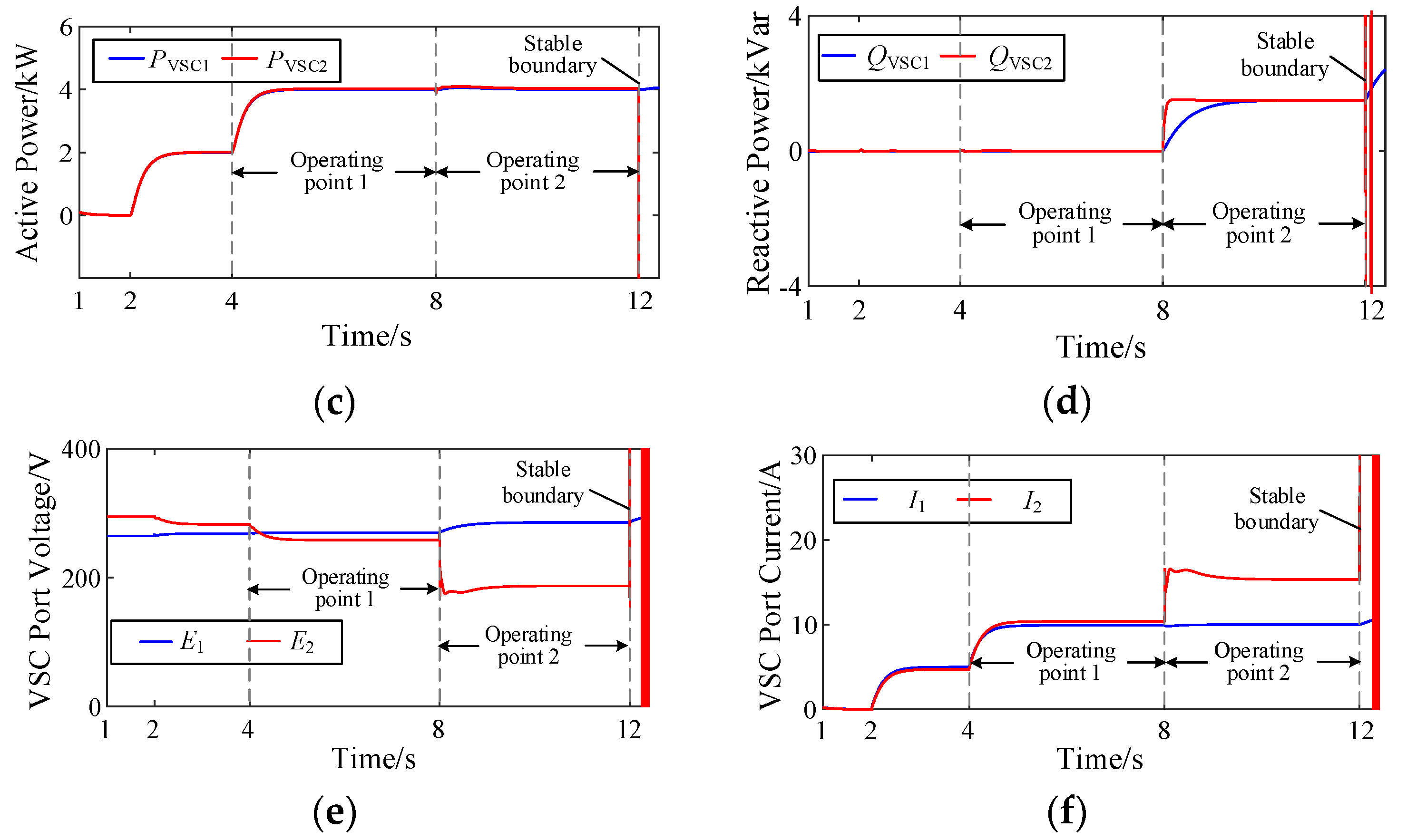
Figure 10 shows the dynamic response curve of the system under the setting of example 1. Through the gradual change in the transmission power reference, the operation state of the BTBC-FMSS is stable at the operating point 1, with PVSC1 = PVSC2 = 4 kW, QVSC1 = QVSC2 = 0 kVar at approximately 6 s, and the synchronization is identified in Figure 9. At 8 s, the reactive power reference of the VSC on both sides is changed to 1.5 kVar, and the operation point of the BTBC-FMSS immediately moves to the right, and finally stabilizes at the operation point 2, with PVSC1 = PVSC2 = 4 kW, QVSC1 = QVSC2 = 1.5 kVar. At 12 s, changing the reactive power reference of VSC on both sides to 3 kVar will cause operating point 2 to continue to move to the right. Due to crossing the stable boundary dominated by VSC2. Looking at Figure 10, we can see that the system becomes unstable immediately after 12 s.
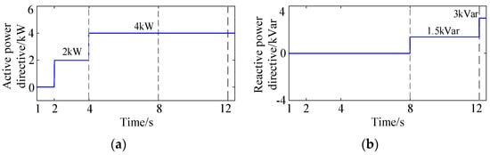
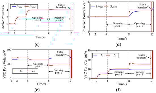
Figure 10.
Dynamic responses of BTBC-FMSS under Case 1: (a) active power directive; (b) reactive power directive; (c) dynamic response of transmitted active power; (d) dynamic response of transmitted reactive power; (e) dynamic response of VSC side voltage; (f) dynamic response of VSC side current.
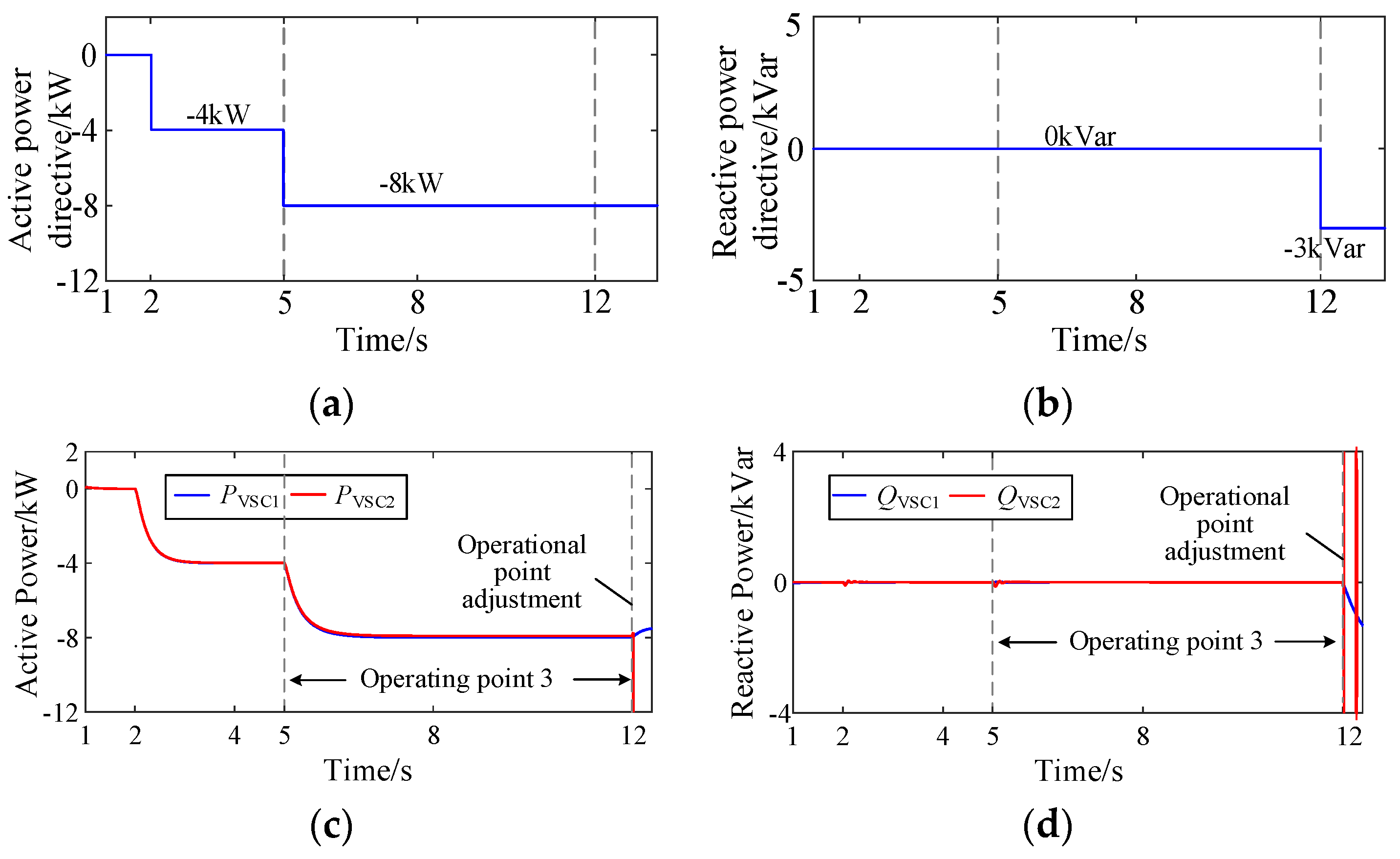
Case 2: All the loads are connected to the system at the beginning of the simulation, and the active and reactive power transmission references are set to 0. For active power control, the active power transmission references are changed to −4 kW and −8 kW at 2 s and 5 s, respectively, and for reactive power control, the reactive power transmission references on both sides of VSC are changed to −3 kVar at 12 s; the simulation ends at 13.5 s.
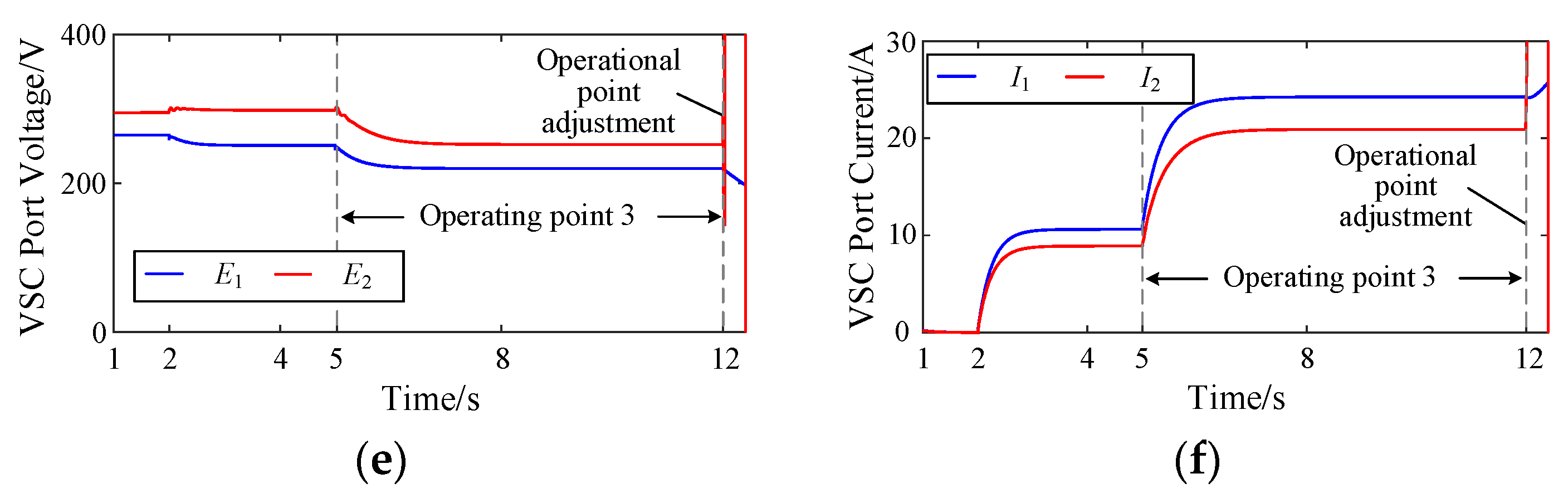
Figure 11 shows the dynamic response curve of each electric quantity of the system under the setting of example 2. Obviously, through the slow change in the active power transmission reference, the operation state of the BTBC-FMSS is stable at operation point 3, with PVSC1 = PVSC2 = −8 kW, QVSC1 = QVSC2 = 0 kVar at approximately 8 s, and the synchronization is identified in Figure 9. At 12 s time, when the reactive power reference is given to −3 kVar, the BTBC-FMSS becomes unstable immediately after 12 s because it crosses the stability boundary dominated by VSC1.

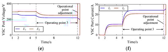
Figure 11.
Dynamic responses of BTBC-FMSS under Case 2: (a) active power directive; (b) reactive power directive; (c) dynamic response of transmitted active power; (d) dynamic response of transmitted reactive power; (e) dynamic response of VSC side voltage; (f) dynamic response of VSC side current.
Case 3: In order to verify the generality and scalability of the proposed method, based on the system in Figure 8, the photovoltaic system, energy storage device and DC load are further added to the DC bus side, and the line and load parameters of the AC side are changed at the same time. The varied system diagram is shown in Figure 12. Ignoring the dynamic of the DC/DC converter, and the equivalent DC component at DC bus can be equivalent to a constant power DC load. To facilitate the analysis, the equivalent constant power DC load is set to 1 kW in the simulation system. The structure and control parameters of the LVDC DN system and the BTBC-FMSS device are shown in Table 4, and the impedance parameters of the distribution lines and loads on both sides are shown in Table 5.
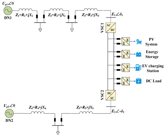
Figure 12.
The simulation circuit diagram of Case 3.
Table 4.
The structure and control parameters of flexible interconnected DN in case 3.
Table 5.
Structural parameters of flexible interconnected distribution grids before and after Davening equivalence in case 3.
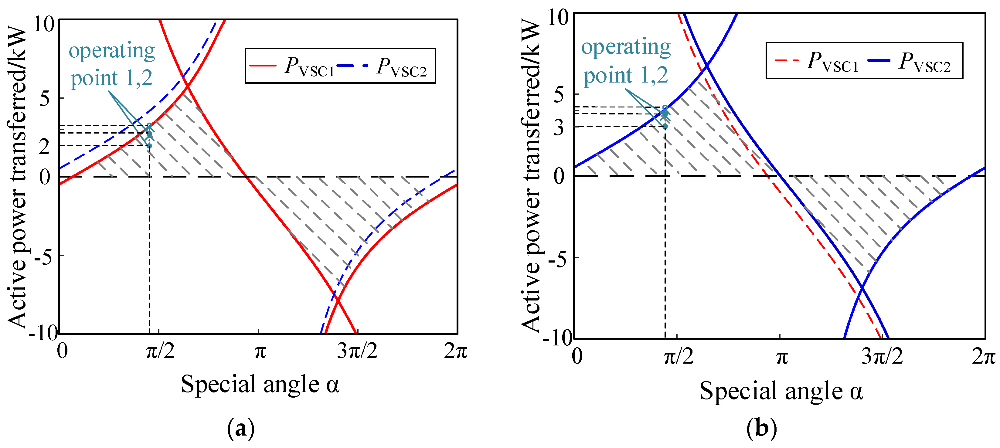
After the load is added to the DC side, the operating states on both sides of BTBC-FMSS will no longer be consistent, and their stable operation domains will also change, but there is always an equation constraint relationship of PVSC1 + Pdc = PVSC2. When the power is transmitted forward and satisfies the inequality PVSC1 + Pdc > PVSC2, the stability boundary of VSC2 side remains unchanged, while the stability operation domain of VSC1 side becomes smaller due to the ‘pinning’ effect of VSC2 side. The stability boundary of VSC1 side is adjusted to the stability boundary of VSC2 side minus the boundary of constant power of DC side. When the power on both sides satisfies the inequality PVSC1 + Pdc < PVSC2, the stable boundary on the VSC1 side remains unchanged, and the stable operation domain on the VSC2 side becomes larger. The specific performance is that the stable boundary on the VSC2 side is adjusted to the stable boundary on the VSC1 side and the boundary after the constant power on the DC side; the opposite is true when the power is transmitted in the reverse direction. The specific stable operation domains on both sides of BTBC-FMSS are shown in Figure 13. The area enclosed by the red curve in Figure 13a is the stable operation domain on the VSC1 side, and the area enclosed by the blue curve in Figure 13b is the stable operation domain on the VSC2 side.
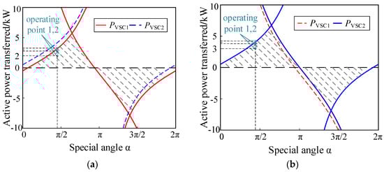
Figure 13.
Stable operation domains of BTBC-FMSS under simulation case 3: (a) stable operation domain on the VSC1 side; (b) stable operation domain on the VSC2 side.
According to Thevenin’s equivalent method, the equivalent impedance parameters of the distribution network on both sides under full load access are Zs1 = 5.06 Ω∠79.24°, Zs2 = 8.68 Ω∠77.84°, Ug1 = 324∠−1.27°, Ug2 = 288.6∠−4.06°, and equivalent voltage.
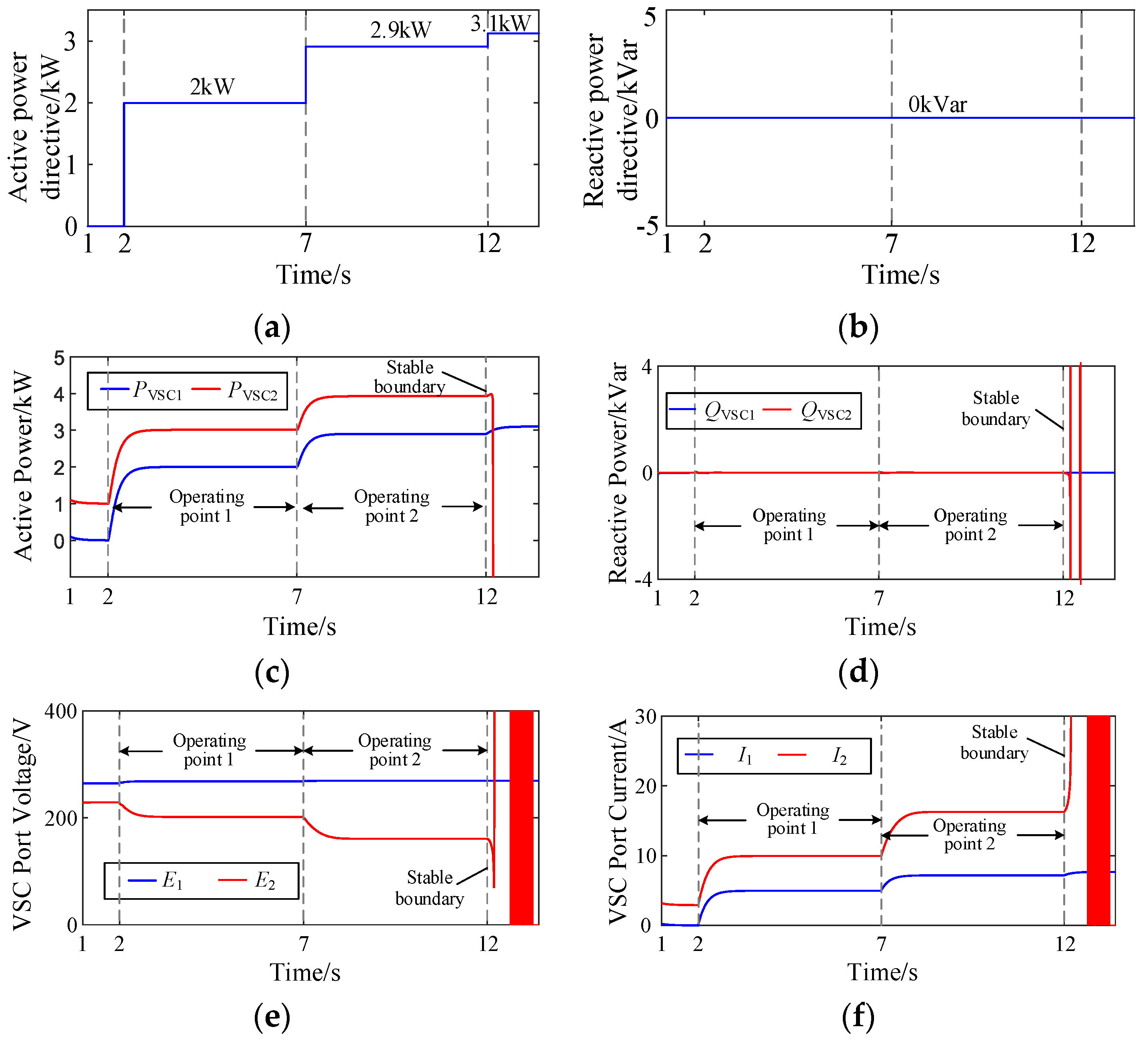
At the beginning of the simulation, all loads are connected to the system, and the active and reactive power transmission references are set to 0. For active power control, the active power transmission command is changed to 2 kW, 2.9 kW and 3.1 kW at 2 s, 7 s and 12 s, respectively. The reactive power reference is always 0; the simulation ends at 12.5 s.
Figure 14 shows the dynamic response curve of each electrical quantity of the system under the setting of example 3. Through the gradual change in the transmission power reference, roughly at 3 s, the VSC1 side is stable at the operating state with PVSC1 = 2 kW, QVSC1 = 0 kVar, and the VSC2 side is stable at the operating state with PVSC2 = 3 kW, QVSC2 = 0 kVar, which is synchronously identified in Figure 13a,b. At 7 s, the active command on the VSC1 side is changed to 2.9 kW. At this time, the operating points on both sides will move upward, and finally stabilize at the operating point 2 of PVSC1 = 2.9 kW, QVSC1 = 0 kVar, PVSC2 = 3.9 kW, QVSC2 = 0 kVar. At 12 s, the active power command on the VSC1 side is increased to 3.1 kW, which causes the operating points on both sides to continue to move upward due to the crossing of the VSC2-dominated stability boundary. It can be seen from Figure 14 that the system is unstable immediately after 12 s. Therefore, the simulation verifies the effectiveness of the BTBC-FMSS stable operation domain under different network topologies, load/generation conditions and parameter settings.

Figure 14.
Dynamic responses of BTBC-FMSS under Case 3: (a) active power directive; (b) reactive power directive; (c) dynamic response of transmitted active power; (d) dynamic response of transmitted reactive power; (e) dynamic response of VSC side voltage; (f) dynamic response of VSC side current.
6. Conclusions
This paper studies the transmission power limit and static stability of the ideal distribution system with BTBC-FMSS access, and draws the following conclusions:
(1) The transmission power limit of BTBC-FMSS is affected by the combined dynamic effects of structural parameters such as grid strength Ugi/|Zsi|, impedance angle θzi and other structural parameters, as well as control parameters such as current amplitude Ii and power factor angle φi on both sides of BTBC-FMSS.
(2) BTBC-FMSS’s two sides of the VSC transmission power limit itself by each side of the PLL static stabilization of the operating point of the existence of this condition constraint; there is a − αi curve for each, and the actual BTBC-FMSS power transmission limit of the − αi curve is the intersection of the two.
(3) The stable operating region of BTBC-FMSS proposed in this paper makes it easier to quantify the stable operating region of the device’s power transfer than the short-circuit ratio or the small-signal stability analysis, and it can guide the capacity configuration and optimal operation of BTBC-FMSS, which has good practical value.
Firstly, the small signal entails a large amount of work to determine the stable operating domain by determining whether each operation point is stable. Secondly, the small signal relies on linearization at the operation point. In contrast, the method proposed in this paper is a large-signal analysis method, which directly derives the stability boundary by mainly considering the dominant stable mode of the outer control loop (PLL control loop). Compared with the existing small-signal analysis methods, the method proposed in this paper is much more intuitive and accurate.
Author Contributions
Conceptualization, X.W.; methodology, J.D.; formal analysis, X.W.; investigation, B.X.; data curation, J.D.; writing—original draft preparation, X.W.; writing—review and editing, Z.Q. and X.M.; supervision, X.M. All authors have read and agreed to the published version of the manuscript.
Funding
This research was funded by State Grid Anhui Electric Power Co. (No. B31205230004).
Data Availability Statement
Data are contained within the article.
Conflicts of Interest
The authors Xunting Wang, Jinjin Ding and Bin Xu were employed by State Grid Anhui Electric Power Research Institute. The remaining authors declare that the research was conducted in the absence of any commercial or financial relationships that could be construed as a potential conflict of interest.
References
- Fuad, K.S.; Hafezi, H.; Kauhaniemi, K.; Laaksonen, H. Soft Open Point in Distribution Networks. IEEE Access 2020, 8, 210550–210565. [Google Scholar] [CrossRef]
- Zhang, G.; Wang, Y.; Peng, B.; Lu, Y.; Qiu, P.; Xu, F.; Wang, C. Multi-objective operation optimization of active distribution network based on three-terminal flexible multi-state switch. J. Renew. Sustain. Energy 2019, 11, 2. [Google Scholar] [CrossRef]
- Li, P.; Ji, J.; Ji, H.; Song, G.; Wang, C.; Wu, J. Self-healing oriented supply restoration method based on the coordination of multiple SOPs in active distribution networks. Energy 2020, 195, 116968. [Google Scholar] [CrossRef]
- Zhou, J.Z.; Ding, H.; Fan, S.; Zhang, Y.; Gole, A.M. Impact of Short-Circuit Ratio and Phase-Locked-Loop Parameters on the Small-Signal Behavior of a VSC-HVDC Converter. IEEE Trans. Power Deliv. 2014, 29, 2287–2296. [Google Scholar] [CrossRef]
- Wang, J.; Zhou, N.; Chung, C.Y.; Wang, Q. Coordinated Planning of Converter-Based DG Units and Soft Open Points Incorporating Active Management in Unbalanced Distribution Networks. IEEE Trans. Sustain. Energy 2020, 11, 2015–2027. [Google Scholar] [CrossRef]
- Aithal, A.; Li, G.; Wu, J.; Yu, J. Performance of an electrical distribution network with Soft Open Point during a grid side AC fault. Appl. Energy 2017, 227, 262–272. [Google Scholar] [CrossRef]
- Tian, Y.; Peng, F.; Wang, Y.; Chen, Z. Coordinative impedance damping control for back-to-back converter in solar power integration system. IET Renew. Power Gener. 2019, 13, 1484–1492. [Google Scholar] [CrossRef]
- Li, P.; Ji, H.; Yu, H.; Zhao, J.; Wang, C.; Song, G.; Wu, J. Combined decentralized and local voltage control strategy of soft open points in active distribution networks. Appl. Energy 2019, 241, 613–624. [Google Scholar] [CrossRef]
- Zhou, J.Z.; Gole, A.M. VSC transmission limitations imposed by AC system strength and AC impedance characteristics. In Proceedings of the 10th IET International Conference on AC and DC Power Transmission (ACDC 2012), Birmingham, UK, 1–5 December 2012; pp. 1–6. [Google Scholar]
- Yuan, H.; Xin, H.; Wu, D.; Li, Z.; Qin, X.; Zhou, Y.; Huang, L. Assessing Maximal Capacity of Grid-Following Converters with Grid Strength Constraints. IEEE Trans. Sustain. Energy 2022, 13, 2119–2132. [Google Scholar] [CrossRef]
- Huang, Y.; Wang, D. Effect of Control-Loops Interactions on Power Stability Limits of VSC Integrated to AC System. IEEE Trans. Power Deliv. 2017, 33, 301–310. [Google Scholar] [CrossRef]
- Huang, S.; Wu, S.; Zhang, J.; Sun, B.; Han, T. Research on and application of fault disposal in flexible interconnection distribution network. In Proceedings of the 2020 IEEE International Conference on Advances in Electrical Engineering and Computer Applications (AEECA), Dalian, China, 25–27 August 2020; pp. 639–642. [Google Scholar]
- He, X.; Geng, H.; Xi, J.; Guerrero, J.M. Resynchronization Analysis and Improvement of Grid-Connected VSCs during Grid Faults. IEEE J. Emerg. Sel. Top. Power Electron. 2019, 9, 438–450. [Google Scholar] [CrossRef]
- He, X.; Tsinghua University; Geng, H.; Ma, S. Transient Stability Analysis of Grid-Tied Converters Considering PLL’s Nonlinearity. CPSS Trans. Power Electron. Appl. 2019, 4, 40–49. [Google Scholar] [CrossRef]
- Hu, Q.; Fu, L.; Ma, F.; Ji, F. Large Signal Synchronizing Instability of PLL-Based VSC Connected to Weak AC Grid. IEEE Trans. Power Syst. 2019, 34, 3220–3229. [Google Scholar] [CrossRef]
- Zhao, Y.; Yang, Q.; Dai, N.; Huang, Y. An improved control strategy with adaptive dynamic reference control for DC voltage stabilization in soft open point. In Proceedings of the 2023 IEEE 2nd International Power Electronics and Application Symposium (PEAS), Guangzhou, China, 10–13 November 2023; pp. 2203–2208. [Google Scholar]
- Song, J.; Zhang, Y.; Gao, Z.; Cao, C.; Wang, Z.; Xu, F. Research on Topology and control technology of soft multi-state open point with fault isolation capability. In Proceedings of the 2018 China International Conference on Electricity Distribution (CICED), Tianjin, China, 17–19 September 2018; pp. 1467–1473. [Google Scholar]
- Göksu, Ö.; Teodorescu, R.; Bak, C.L.; Iov, F.; Kjær, P.C. Instability of Wind Turbine Converters During Current Injection to Low Voltage Grid Faults and PLL Frequency Based Stability Solution. IEEE Trans. Power Syst. 2014, 29, 1683–1691. [Google Scholar] [CrossRef]
- Naderi, M.; Khayat, Y.; Shafiee, Q.; Dragicevic, T.; Bevrani, H.; Blaabjerg, F. Interconnected Autonomous AC Microgrids via Back-to-Back Converters—Part I: Small-Signal Modeling. IEEE Trans. Power Electron. 2019, 35, 4728–4740. [Google Scholar] [CrossRef]
- Naderi, M.; Khayat, Y.; Shafiee, Q.; Dragicevic, T.; Bevrani, H.; Blaabjerg, F. Interconnected Autonomous ac Microgrids via Back-to-Back Converters-Part II: Stability Analysis. IEEE Trans. Power Electron. 2020, 35, 11801–11812. [Google Scholar] [CrossRef]


Disclaimer/Publisher’s Note: The statements, opinions and data contained in all publications are solely those of the individual author(s) and contributor(s) and not of MDPI and/or the editor(s). MDPI and/or the editor(s) disclaim responsibility for any injury to people or property resulting from any ideas, methods, instructions or products referred to in the content. |
© 2024 by the authors. Licensee MDPI, Basel, Switzerland. This article is an open access article distributed under the terms and conditions of the Creative Commons Attribution (CC BY) license (https://creativecommons.org/licenses/by/4.0/).