A Nonlinear Hybrid Modeling Method for Pump Turbines by Integrating Delaunay Triangulation Interpolation and an Improved BP Neural Network

Abstract

In order to solve the problem that the data processing accuracy of the characteristic curves is not high, which affects the accuracy of the simulation of variable-speed pumped storage units, this paper proposes a nonlinear hybrid modeling method for pump turbines by integrating Delaunay triangulation interpolation and an improved back-propagation neural network. Firstly, the improved Sutter transform is used to preprocess the original curve, and the convex hull of the transformed curve is calculated. With the unknown point inside the convex hull, Delaunay triangulation interpolation is used to model the transformed curve. With the unknown point outside the convex hull, the back-propagation neural network is first established based on the input and output, and then the initial weights and thresholds of the network are determined using the mind evolution algorithm to complete the modeling and simulation of the curve. Simulation results show that the proposed method fully integrates the high-precision features of interpolation and the powerful nonlinear fitting ability of the neural network, which greatly improves the efficiency and accuracy of pump turbine modeling.

1. Introduction

With the continuous development of the power industry and the demand for clean, low-carbon, and green development, renewable energy represented by hydropower has developed rapidly [1,2,3]. Among them, variable-speed pumped storage units (VSPSUs) based on doubly fed induction motors and pump turbines (PTs) have become a research hotspot in recent years due to their advantages of large capacity, high operating efficiency, and flexible power adjustment [4,5,6]. Different from conventional fixed-speed pumped storage units, VSPSUs can continuously adjust the pump power by adjusting the speed under the pump condition, and the operating efficiency of the PT will change with the change in head and speed [7,8]. Therefore, in order to realize accurate simulation calculations, it is urgent to study and establish a high-precision model of PTs while laying the foundation for the optimal working condition tracking and optimization control of VSPSUs [9].

The modeling of a PT is mainly to obtain the mathematical relationship between the unit’s quantity of flow, torque and opening, speed, and working head. So far, its mathematical models can be broadly divided into three categories, namely linear models [10,11,12,13], nonlinear models proposed by the IEEE PES Working Group [14,15], and nonlinear models based on characteristic curves [16,17,18,19,20,21,22,23]. The linear model simply performs a Taylor expansion of the torque and flow formulas, ignoring the second-order and higher-order derivative terms. Although linear models are simple and easy to solve, they cannot accurately describe the characteristics of the PT [16]. On the premise of ignoring the loss, the IEEE PES Working Group proposed nonlinear models for hydraulic turbines, taking into account factors such as opening, head, and quantity of flow [14]. In engineering practice and theoretical research, complete characteristic curves of a PT are easy to obtain, and they can also fully describe the nonlinear characteristics. Therefore, using characteristic curves is the most direct and detailed method to reflect the relationship between parameters under various operating conditions of the unit [16].

The modeling based on characteristic curves has always used traditional interpolation and neural network methods. In [17], the comprehensive characteristic data were interpolated using triangulation, and the results were verified to be unique and correct through experiments. In [18], a turbine model was established using a back-propagation (BP) neural network. In [19], a deep learning method based on improved particle swarm optimization and long short-term memory was proposed to fit the flow curve of the turbine, and the effectiveness of the method was verified. However, the complete characteristic curves exhibit an S-shape in the runaway and reverse pump conditions, and there are also intersections and overlaps in the working area of the pump. This brings significant difficulties to the fitting and modeling of the characteristic curves. In order to fully estimate the curves, researchers usually use methods such as the Sutter transform and its improvement, as well as three-dimensional curve fitting. The Sutter transform proposed in [21] converts the original curve into a curve with a small twist and no multi-value curve, which solves the difficulty of fitting to a certain extent. On this basis, an improved Sutter transform method was proposed to process the curves, and the transformed curves were fitted by least squares, which provided convenience for the calculation of the PT [22]. Based on the improved Sutter transform, an extreme learning machine model based on a novel autoencoder was proposed in [23]. The research results show that the model has better modeling accuracy and generalization ability than the traditional neural network model.

In fact, the spatial interpolation algorithm is accurate enough—even higher than the fitting accuracy of general neural networks—to complete high-precision modeling of the PT. However, it cannot interpolate in the blank data area of the boundary. Obviously, it is not enough to build a pump turbine model based on interpolation or neural networks.

Based on the above analysis, this paper first preprocesses the original characteristic curve using the improved Sutter transform in order to improve the modeling accuracy of the PT. Then, within the convex hull, the transformed curve is interpolated using Delaunay triangulation interpolation. Beyond the convex hull, the mind evolutionary algorithm is used to optimize the initial weights and thresholds of the back-propagation (BP) neural network, and then the improved BP (IBP) is used to fit and expand the transformed curve. Finally, the modeling under all working conditions is complete. In this paper, three experiments (convex hull inner, convex hull outer, and partially convex hull outer) were carried out, using BP, IBP, convolutional neural network (CNN), long short-term memory (LSTM), and random forest (RF) models as comparative models. The experimental results show that: (1) when the test set is all within the convex hull, the modeling accuracy of the proposed method and the interpolation method is the highest; (2) when the test set is all outside the convex hull, the proposed method and IBP have the highest modeling accuracy; (3) when part of the test set is outside the convex hull, the modeling accuracy of the proposed method is the highest. In addition, the results of the Friedman test in Experiment 3 verify that the proposed method is significantly different from the comparison method, and the performance of this method ranks first.

2. Modeling and Modeling Evaluation of the PT

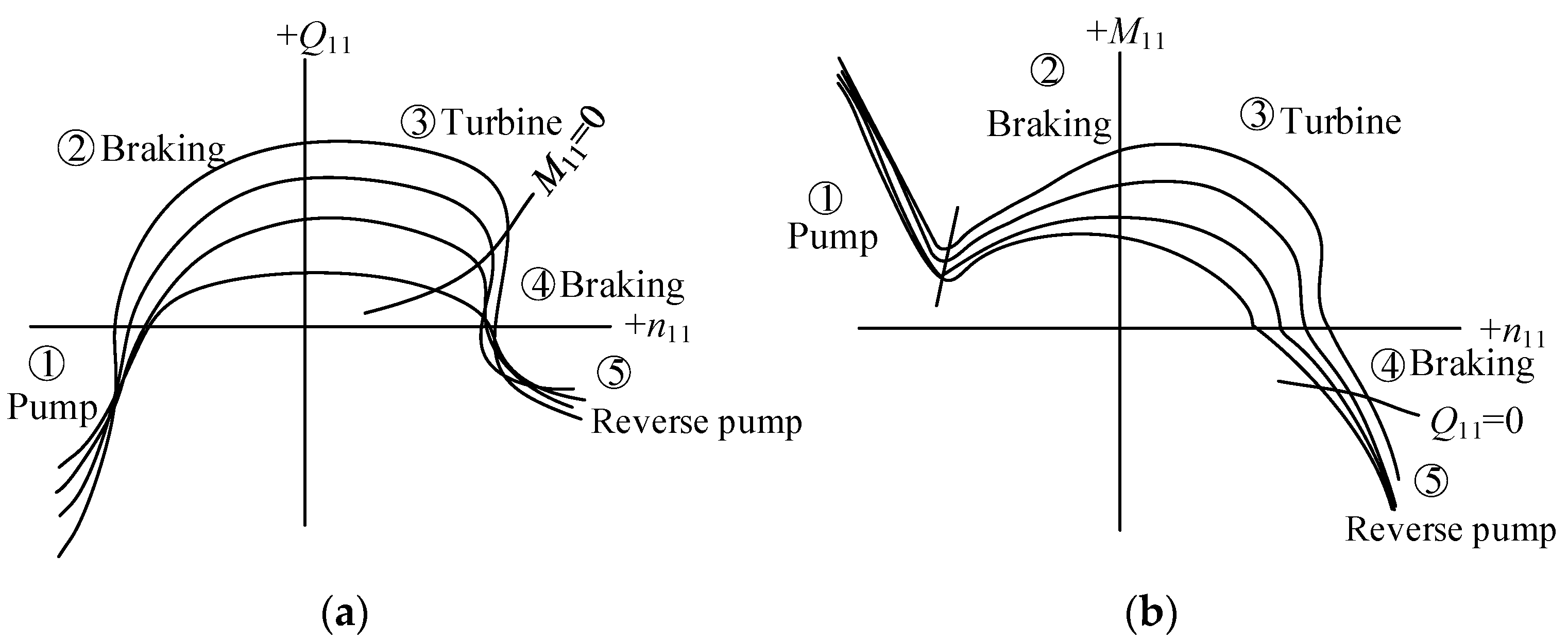
2.1. Modeling of the PT Based on the Complete Characteristic Curve

The pump turbine is a complex nonlinear system, and there is currently no recognized analysis formula to describe the quantity of flow and torque. The commonly used method is to discretize the complete characteristic curve and model it using numerical calculation methods. According to the IEC-60193 specification [24], the complete four-quadrant characteristic curve of the impeller can be obtained through model testing, as shown in Figure 1.

The complete characteristic curves include the flow characteristic curve and torque characteristic curve, which describe the nonlinear relationship between the unit quantity of flow, unit torque, unit speed, and opening, as shown in (1).

$$\{\begin{array}{c}{Q}_{11}=f_Q(y,n_{11}) \\ M_{11}=f_M(y,n_{11})\end{array}$$

(1)

where $Q_{11}$, $M_{11}$, and $n_{11}$ are the unit flow, unit speed, and unit torque, respectively, and y is the opening. $f_Q$ represents a nonlinear function of unit flow rate, unit speed, and opening, while $f_M$ represents a nonlinear function of unit torque, unit speed, and opening.

It can be clearly seen from Figure 1 that the same set of unit speeds and openings at both ends of the curve correspond to three or more flows and torques, and there is a multi-value problem. In order to solve that problem, relevant scholars have proposed a series of curve transformation methods. The improved Sutter transformation method proposed in [25] effectively solves the problem. Therefore, this paper adopts this method, and the formula is as follows:

$$\{\begin{array}{l}WH(x,y)=\frac{h}{{\alpha }^2+q^2+C_h\cdot h}{\left(y+C_y\right)}^2\\ WM(x,y)=\left(\frac{m+k_{1}h}{{\alpha }^2+q^2+C_h\cdot h}\right){\left(y+C_y\right)}^2\\ x=\arctan \left[\left(q+k_2\sqrt{h}\right)/\alpha \right],\alpha >0\\ x=\pi +\arctan \left[\left(q+k_2\sqrt{h}\right)/\alpha \right],\alpha <0\end{array}$$

(2)

where k₁ > |M_11max|/M_11r, k₂ = 0.5~1.2, C_y = 0.1~0.3, and C_h = 0.4~0.6.

Therefore, by determining the WH curve and WM curve with small torsion and no multiple values, the complete characteristic curve can be deduced. Modeling the pump turbine is transformed into modeling the WH and WM curves.

2.2. Modeling Evaluation Indicators

In order to objectively understand the accuracy of modeling, this paper uses root mean square error (RMSE), mean absolute percentage error (MAPE), and coefficient of decision (R²) to verify the feasibility and effectiveness and compare the effects of different modeling methods based on these values. Their expressions are as follows:

$$\{\begin{array}{l}RMSE=\sqrt{\frac{1}{N}{\displaystyle \sum _{i=1}^N{({\widehat{y}}_i-y_i)}^2}}\\ MAPE=\frac{1}{N}{\displaystyle \sum _{i=1}^N\left|\frac{{\widehat{y}}_i-y_i}{y_i}\right|}\\ R^2=1-{\displaystyle \sum _{i=1}^N{({\widehat{y}}_i-y_i)}^2}/{\displaystyle \sum _{i=1}^N{({\widehat{y}}_i-\overline{y})}^2}\end{array}$$

(3)

where $y=[y_1,y_2,\cdots ,y_N]$ and $\widehat{y}=[{\widehat{y}}_1,{\widehat{y}}_2,\cdots ,{\widehat{y}}_N]$ are the actual series and the modeled estimated series, respectively, and $\overline{y}$ is the average value of y.

3. Nonlinear Hybrid Modeling Method for the PT

In order to ensure the accuracy of modeling, this paper combines the high-precision features of interpolation with the powerful nonlinear fitting ability of a neural network. Next, we will introduce Delaunay triangulation interpolation, improved BP (IBP) optimized by the mind evolutionary algorithm, and a nonlinear hybrid modeling method.

3.1. Delaunay Triangulation Interpolation

Triangulation essentially organizes scattered points in a plane or space, expressing adjacency relationships through triangles or tetrahedrons, as shown in Figure 2.

Delaunay triangulation is the most classic method for triangulation, and it has been proven to be the most optimized triangulation.

There are two types of algorithms for Delaunay triangulation. One is the incremental algorithm, and commonly used algorithms include Green-Sibson [26], Lawson [27], etc. Another type is the divide-and-conquer algorithm [28]. Taking the Lawson algorithm as an example, the principle of Delaunay triangulation will be introduced below.

(1)

A super triangle containing all the measurement points is constructed and placed in a linked list of triangles.

(2)

The measurement points in the set are sequentially inserted. First, the triangle containing the insertion point in the circumcircle is identified. The insertion point is then connected to all the vertices of the triangle, completing the insertion of a point in the Delaunay triangle linked list.

(3)

Based on the characteristics of the Delaunay triangulation network’s external empty circles, the optimization criterion is used to optimize the newly formed local triangle to satisfy the Delaunay characteristics.

(4)

Steps (2)–(4) above are performed in a loop until all measurement points have been inserted, forming a complete irregular network.

(5)

Similarly, the points to be interpolated need to follow step (4), and the estimated values of the points can be calculated through linear interpolation.

Obviously, the points to be interpolated need to be inserted into the Delaunay triangular irregular network and cannot be interpolated in the blank data area of the boundary.

3.2. IBP Optimized by the Mind Evolutionary Algorithm

The initial weight and threshold of the neural network are related to training speed, convergence rate, and convergence effect. In this paper, the mind evolutionary algorithm (MEA) is used to optimize the BP for the nonlinear modeling of pump turbines. The detailed optimization steps are as follows:

(1) The BP neural network [29] corresponding to the input and output is established, and a population containing weights and thresholds is generated for training the network. Firstly, R sets of data are randomly generated as initial values for the population, which follows a uniform distribution between (0,1). The root mean square difference between the objective function and the network output value is calculated as the score for each individual.

$${\xi }_{AV}=\frac{1}{2s}{\displaystyle \sum _{n=1}^s{\displaystyle \sum _{j=1}^q{(d_j(n)-y_j(n))}^2}}$$

(4)

where s is the total number of training samples, $d_j(n)$ is the value of the objective function, and $y_j(n)$ is the output data of the network. The smaller the $d_j(n)-y_j(n)$, the better the weight and threshold data contained by the individual, and the better the individual’s score. Then M + T individuals with the best scores from the population are selected, including the M superior subpopulation and the T temporary subpopulation.

(2) Convergence operations are carried out within the population. Taking each winner as the center, M superior subpopulations and T temporary subpopulations are generated by using the normal distribution $N(\mu ,\Sigma )$. When each vector is independent of each other, its diagonal element is assumed to be $\left\{{\sigma }_{id}\right\},d=0,1,\cdots ,R$. When the population evolves, the weight or threshold of the winner is taken as the mean, and the covariance of the new generation of sub-individuals is:

$$\{\begin{array}{c}{\sigma }_{(i+1)d}=c_1{\sigma }_{id}+c_2\delta \\ \delta =\sqrt{{\displaystyle \sum _{j=1}^R({{\mu }^{\prime }}_j-{\mu }_j)}}\end{array}$$

(5)

where $c_1$ and $c_2$ are constants between 0.1 and 0.5, and $\delta$ is the difference between the two generations of winners.

(3) The alienation operation between populations is carried out. The alienation of the MEA takes place throughout global space. According to the score, the replacement of the winning subpopulation and the temporary subpopulation, the abandonment of the temporary subpopulation, and the release and reorganization of the subpopulation are completed.

(4) Convergence is judged, and if the conditions are not met, steps (2) and (3) are performed repeatedly.

3.3. Nonlinear Hybrid Modeling Method

Considering the shortcomings of Delaunay triangulation interpolation and the strong nonlinear fitting ability of IBP, this paper proposes a nonlinear hybrid modeling method for pump turbines by intergrating Delaunay triangulation interpolation and improved BP, as shown in Figure 3. Within the convex hull, Delaunay triangulation is used to interpolate and encrypt the curves. In addition to the convex hull, the mind evolutionary algorithm is used to optimize the initial weight and threshold of the BP, and the data of the unknown region are estimated by the smooth extension of the IBP.

4. Experimental Verification

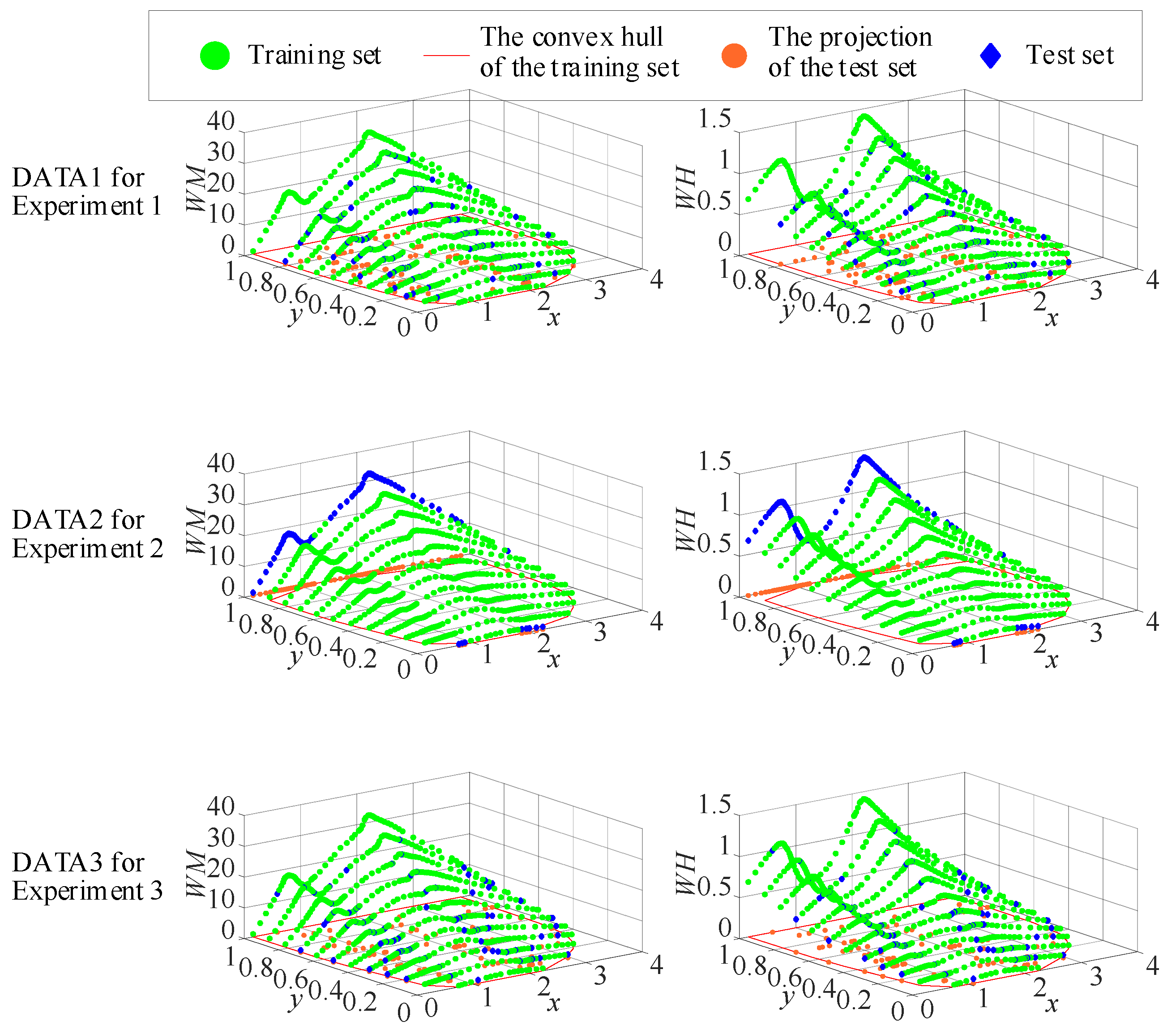
4.1. Experimental Data

In this paper, the complete characteristic curve of a pump turbine is selected as the experimental data, as shown in Figure 4a,b, which contains a total of 891 sets of data. First, the original data are processed according to (2) to obtain new data, and the WH and WM curves are shown in Figure 4c,d. It is worth mentioning that in (2), k₁ = 19.5, k₂ = 0.9, C_y = 0.2, and C_h = 0.5. As shown in Figure 4, the improved Sutter transform transforms the original curve with large torsion and multiple values into the WH curve and the WM curve with small torsion and no multiple values. Modeling a pump turbine essentially translates to modeling WH and WM curves.

In order to test the effectiveness of the proposed method, this paper divides the training set and the test set of the data according to 9:1. Among them, 801 sets of data are used to train the model, and 90 sets of data are used to test the model. In order to fully validate the effectiveness, three sets of experiments are designed in this paper, and the experimental data are shown in Figure 5. It depicts three sets of experimental data, where the green part is the training set, the red curve is the convex hull of the training set, the blue part is the test set, and the orange part is the projection of the test set. As can be seen from Figure 5, all the test sets in experiment 1 are inside the convex hull, all the test sets in experiment 2 are outside the convex hull, and part of the test sets in experiment 3 are inside the convex hull, while some are outside the convex hull.

4.2. Experiment 1: Inside the Convex Hull

Taking DATA1 in Figure 5 as the experimental data, the hybrid modeling method in Figure 3 is used to establish the pump turbine model. The training set is used for model training, and the test set is used for validating the effectiveness of the model. Figure 6 shows the error of the model estimation results for the test set, where interpolation (IP), BP, IBP, convolutional neural network (CNN), long short-term memory (LSTM), and random forest (RF) are used as comparison methods. Figure 6 is a biaxial graph, where the gray part represents RMSE, with the left axis as the vertical axis. Blue and red, respectively, represent MAPE and 1-R², with the right axis as the vertical axis.

As can be seen from Figure 6, among the methods, the estimation error of the interpolation and the proposed hybrid method (PHM) is consistent and minimal, and their determination coefficients are closest to 1, which are 99.993% (WH) and 99.996% (WM). On the one hand, the reason why they have the same result is that the test set in DATA1 is all within the convex hull of the training set, and the PHM is essentially an interpolation method in this example. On the other hand, the results in Figure 6 also show that the interpolation method has the highest modeling accuracy when it is within the convex hull. In addition, the estimation error of WH shows that IBP greatly improves the accuracy of BP, and the RMSE is reduced from 0.06 to 0.032, MAPE is reduced from 8.161% to 4.704%, and R² is increased from 94.7363% to 98.5383%. In addition, in the neural network method, RF performed best in WH modeling, while BP and IBP performed best in WM modeling, and CNN and LSTM did not perform particularly well in this experiment. This may be due to the fact that LSTM and CNN, as representatives of deep learning, have strong applicability to long-term dependence and spatial data, while the modeling of the PT does not have these characteristics itself, so the modeling effect of deep learning is not as good as that of shallow neural networks.

4.3. Experiment 2: Outside the Convex Hull

Using DATA2 in Figure 5 as the experimental data, the model estimation error of the test set is shown in Figure 7. It is worth mentioning that for cases where interpolation outside the convex hull cannot obtain effective results, this paper replaces it with the average of the effective results in the test set.

From Figure 7, it can be seen that the estimation errors of IBP and the PHM are consistent and minimal among all methods, and R² is closest to 1, with values of 99.133% (WH) and 99.774% (WM). On the one hand, the reason why they have the same result is that the test set in DATA2 is all outside the convex hull of the training set, and the PHM is essentially an IBP method in this example. On the other hand, the results in Figure 7 also show that IBP has the highest modeling accuracy outside the convex hull. In addition, it can be clearly seen in Figure 7 that in both WH and WM modeling, the IBP modeling error in this paper is the lowest and the accuracy is the highest, while the accuracy of RF is the lowest. The above analysis fully proves the superiority of IBP in solving the problem that interpolation cannot obtain effective results.

4.4. Experiment 3: Partially Outside the Convex Hull

Using DATA3 in Figure 5 as the experimental data, the model estimation error of the test set is shown in Figure 8.

As can be seen from Figure 8, the estimation error of the PHM in this paper is the smallest, and the R² is closest to 1. This is because the PHM fully combines the advantages of the interpolation method and the IBP method in different scenarios. Overall, RF performs poorly in modeling, which may be due to the fact that RF is not able to make estimates beyond the scope of the training set of data when performing regression, which can lead to transitional fitting when modeling data outside of the training set. This can be demonstrated by the RF estimation error in Figure 6, Figure 7 and Figure 8.

In fact, after obtaining the WH and WM modeling estimation results, it is necessary to calculate the unit torque according to Equation (2). Based on the above results, the estimation result of the unit torque is shown in Figure 9, and the estimation error is shown in

Table 1. The estimation error.

	Error	RMSE	MAPE (%)	R2 (%)
Model
IP		3160.3143	88.4499	9.4724
BP		244.8342	7.8279	95.9455
IBP		196.9613	3.3978	94.5856
CNN		268.3546	9.9853	93.4788
LSTM		482.9481	11.8363	79.2922
RF		475.0019	20.1417	80.5958
PHM		152.2848	3.4479	97.6663

.

As can be seen from Figure 9 and Table 1, the PHM in this paper has the highest modeling accuracy, with the lowest RMSE and MAPE, and R² is closest to 1. By carefully observing Table 1 and Figure 6, Figure 7 and Figure 8, it can be seen that the modeling accuracy of the unit torque is lower than that of WH and WM, especially the interpolation method. This is why, even in the case of high modeling accuracy of WH and WM curves, it is still necessary to further integrate IBP to improve the accuracy of modeling.

Furthermore, the non-parametric Friedman test method is used to verify the difference between the estimated results of several models, and the model effects are ranked. The calculated results of the Friedman test are shown in

Table 2. The Friedman test results.

Model	IP	BP	IBP	CNN	LSTM	RF	PHM
Mean rank	2.5611	3.8556	4.1833	5.2222	4.9556	4.9444	2.2778
Sort	2	3	4	7	6	5	1
p-value	p = 5.8487 × 10−33

.

The p < 0.01 in Table 2 shows that there is a significant gap between the estimation results of these seven models at the significant level of 0.01. According to the ranking of the mean rank, the PHM ranks first, which also shows the effectiveness of the proposed method in this paper. It is worth mentioning that the interpolation ranks second only to the PHM, which is inconsistent with the lowest correlation coefficient of the interpolation method in Table 1. This is because nonparametric tests are essentially sorting-based statistical methods that compare the average performance of multiple models. The low performance of certain test points has a low impact on the overall performance ranking.

5. Conclusions

In this paper, a nonlinear hybrid modeling method for pump turbines is proposed by combining the high-precision features of interpolation with the strong nonlinear fitting ability of a neural network. First, the improved Sutter transform is used to solve the multi-value problem, and the original characteristic curves are transformed into the WH curve and WM curve with small torsion and no multi-value. Then, the convex hull of the transformed curve is calculated, and the curve is modeled using Delaunay triangulation interpolation or BP optimized by the mind evolutionary algorithm by judging whether the test point is in the convex hull. Compared with the common BP, CNN, LSTM, and RF, the proposed method significantly improves the modeling efficiency and accuracy of pump turbines.

Considering that the proposed method has good results in the modeling of pump turbines, the next research work will continue to cut in from this perspective and discuss how to achieve optimal working condition tracking and coordinated control of variable-speed pumped storage units based on the high-precision pump turbine model.

References

1. 2023 Statistical Review of World Energy[EB/OL]//Energy Institute. Available online: https://www.energyinst.org/statistical-review (accessed on 18 January 2024).
2. European Electricity Review 2022[EB/OL]//Ember. Available online: https://ember-climate.org/insights/research/european-electricity-review-2022/#supporting-material (accessed on 18 January 2024).
3. Hoffstaedt, J.P.; Truijen, D.P.K.; Fahlbeck, J.; Gans, L.H.A.; Qudaih, M.; Laguna, A.J.; De Kooning, J.D.M.; Stockman, K.; Nilsson, H.; Storli, P.-T.; et al. Low-head pumped hydro storage: A review of applicable technologies for design, grid integration, control and modelling. Renew. Sustain. Energy Rev. 2022, 158, 112119. [Google Scholar] [CrossRef]
4. Xu, Z.; Deng, C.; Yang, Q. Flexibility of variable-speed pumped-storage unit during primary frequency control and corresponding assessment method. Int. J. Electr. Power Energy Syst. 2023, 145, 108691. [Google Scholar] [CrossRef]
5. Chazarra, M.; Perez-Diaz, J.I.; Garcia-Gonzalez, J. Optimal Joint Energy and Secondary Regulation Reserve Hourly Scheduling of Variable Speed Pumped Storage Hydropower Plants. IEEE Trans. Power Syst. 2018, 33, 103–115. [Google Scholar] [CrossRef]
6. Xu, Z.; Deng, C.; Yang, Q. A primary frequency control strategy for variable-speed pumped-storage plant in generating mode based on adaptive model predictive control. Electr. Power Syst. Res. 2023, 221, 109356. [Google Scholar] [CrossRef]
7. Yao, W.; Deng, C.; Li, D.; Chen, M.; Peng, P.; Zhang, H. Optimal Sizing of Seawater Pumped Storage Plant with Variable-Speed Units Considering Offshore Wind Power Accommodation. Sustainability 2019, 11, 1939. [Google Scholar] [CrossRef]
8. Liu, M.; Tan, L.; Cao, S. Theoretical model of energy performance prediction and BEP determination for centrifugal pump as turbine. Energy 2019, 172, 712–732. [Google Scholar] [CrossRef]
9. Wang, L.; Zhang, K.; Zhao, W. Nonlinear Modeling of Dynamic Characteristics of Pump-Turbine. Energies 2022, 15, 297. [Google Scholar] [CrossRef]
10. Feng, C.; Mai, Z.; Wu, C.; Zheng, Y.; Zhang, N. Advantage of battery energy storage systems for assisting hydropower units to suppress the frequency fluctuations caused by wind power variations. J. Energy Storage 2024, 78, 109989. [Google Scholar] [CrossRef]
11. Chen, Y.; Xu, W.; Liu, Y.; Bao, Z.; Mao, Z.; Rashad, E.M. Modeling and Transient Response Analysis of Doubly-Fed Variable Speed Pumped Storage Unit in Pumping Mode. IEEE Trans. Ind. Electron. 2023, 70, 9935–9947. [Google Scholar] [CrossRef]
12. Mohale, V.; Chelliah, T.R.; Hote, Y.V. Small Signal Stability Analysis of Damping Controller for SSO Mitigation in a Large Rated Asynchronous Hydro Unit. IEEE Trans. Ind. Appl. 2023, 59, 4914–4923. [Google Scholar] [CrossRef]
13. Chen, Y.; Deng, C.; Zhao, Y. Coordination Control between Excitation and Hydraulic System during Mode Conversion of Variable Speed Pumped Storage Unit. IEEE Trans. Power Electron. 2021, 36, 10171–10185. [Google Scholar] [CrossRef]
14. Group, I.W. Hydraulic turbine and turbine control model for system dynamic studies. IEEE Trans. Power Syst. 1992, 7, 167–179. [Google Scholar]
15. Sarasúa, J.I.; Pérez-Díaz, J.I.; Wilhelmi, J.R.; Sánchez-Fernández, J.Á. Dynamic response and governor tuning of a long penstock pumped-storage hydropower plant equipped with a pump-turbine and a doubly fed induction generator. Energy Convers. Manag. 2015, 106, 151–164. [Google Scholar] [CrossRef]
16. Zhao, Z.; Yang, J.; Yang, W.; Hu, J.; Chen, M. A coordinated optimization framework for flexible operation of pumped storage hydropower system: Nonlinear modeling, strategy optimization and decision making. Energy Convers. Manag. 2019, 194, 75–93. [Google Scholar] [CrossRef]
17. Zhang, R.; Liu, Z.; Wang, L.; Zhang, Y. Data interpolation by Delaunay triangulation for the combined characteristic curve of a turbine. J. Hydroelectr. Eng. 2011, 30, 197–952. [Google Scholar]
18. Li, J.; Chen, Q.; Chen, G. Study on synthetic characteristic curve processing of Francis turbine conbined with BP neural network. J. Hydroelectr. Eng. 2015, 34, 182–188. [Google Scholar]
19. Pan, H.; Hang, C.; Feng, F.; Zheng, Y.; Li, F. Improved Neural Network Algorithm Based Flow Characteristic Curve Fitting for Hydraulic Turbines. Sustainability 2022, 14, 10757. [Google Scholar] [CrossRef]
20. Cao, R.; Guo, W.; Qu, F. Hydraulic disturbance characteristics and power control of pumped storage power plant with fixed and variable speed units under generating mode. J. Energy Storage 2023, 72, 108298. [Google Scholar] [CrossRef]
21. Suter, P. Representation of Pump Characteristics for Calculation of Water Hammer. Sulzer Tech. Rev. 1966, 4, 45–48. [Google Scholar]
22. Dorfler, P.K. Improved Suter Transform for Pump-Turbine Characteristics. Int. J. Fluid Mach. Syst. 2010, 3, 332–341. [Google Scholar] [CrossRef]
23. Zhang, C.; Peng, T.; Zhou, J.; Ji, J.; Wang, X. An Improved Autoencoder and Partial Least Squares Regression-Based Extreme Learning Machine Model for Pump Turbine Characteristics. Appl. Sci. 2019, 9, 3987. [Google Scholar] [CrossRef]
24. IEC60193 1999; Hydraulic Turbines, Storage Pumps and Pump-Turbines–Model Acceptance Tests. European Committee for Standards: Brussels, Italy, 1991; Second edition 11-1999.
25. Liu, Z.-M.; Zhang, D.-H.; Liu, Y.-Y.; Zhang, X. New Suter-transformation Method of Complete Characteristic Curves of Pump-turbines Based on the 3-D Surface. China Rural. Water Hydropower 2015, 1, 143–145+150+157. [Google Scholar]
26. Weatherill, N.P.; Hassan, O. Efficient three-dimensional Delaunay triangulation with automatic point creation and imposed boundary constraints. Int. J. Numer. Methods Eng. 2010, 37, 2005–2039. [Google Scholar] [CrossRef]
27. Waston, D.F. Computing the n-dimensional Delaunay tessellation with application to voronoi polytopes. Comput. J. 1981, 24, 167–172. [Google Scholar]
28. Joe, B. Three-Dimensional Triangulations from Local Transformations. Siam J. Sci. Stat. Comput. 1989, 10, 718–741. [Google Scholar] [CrossRef]
29. Yang, W.X.; Tse, P.W. Development of an advanced noise reduction method for vibration analysis based on singular value decomposition. Ndt Int. 2003, 36, 419–432. [Google Scholar] [CrossRef]
Figure 1. Complete characteristic curve of a pump turbine. (a) Flow characteristic curves; (b) torque characteristic curves.
Electronics 13 02573 g001
Figure 2. Triangulation of 2D scattered points.
Electronics 13 02573 g002
Figure 3. Nonlinear hybrid modeling method.
Electronics 13 02573 g003
Figure 4. The complete characteristic curve and the corresponding curves after the improved Sutter transform.
Electronics 13 02573 g004
Figure 5. Experimental data.
Electronics 13 02573 g005
Figure 6. The estimation error of the DATA1 dataset.
Electronics 13 02573 g006
Figure 7. The estimation error of the DATA2 dataset.
Electronics 13 02573 g007
Figure 8. The estimation error of the DATA3 dataset.
Electronics 13 02573 g008
Figure 9. Estimation results for the unit torque.
Electronics 13 02573 g009