Article

A Novel Feature Selection Strategy Based on the Harris Hawks Optimization Algorithm for the Diagnosis of Cervical Cancer

1
Division of Electrical Engineering and Computer Science, Graduate School of Natural Science & Technology, Kanazawa University, Kakuma-Machi, Kanazawa 920-1192, Japan
2
Faculty of Electrical, Information and Communication Engineering, Kanazawa University, Kakuma-Machi, Kanazawa 920-1192, Japan
*
Author to whom correspondence should be addressed.
Electronics 2024, 13(13), 2554; https://doi.org/10.3390/electronics13132554
Submission received: 24 April 2024 / Revised: 11 June 2024 / Accepted: 24 June 2024 / Published: 28 June 2024

Abstract

:
Cervical cancer is the fourth most commonly diagnosed cancer and one of the leading causes of cancer-related deaths among females worldwide. Early diagnosis can greatly increase the cure rate for cervical cancer. However, due to the need for substantial medical resources, it is difficult to implement in some areas. With the development of machine learning, utilizing machine learning to automatically diagnose cervical cancer has currently become one of the main research directions in the field. Such an approach typically involves a large number of features. However, a portion of these features is redundant or irrelevant. The task of eliminating redundant or irrelevant features from the entire feature set is known as feature selection (FS). Feature selection methods can roughly be divided into three types, including filter-based methods, wrapper-based methods, and embedded-based methods. Among them, wrapper-based methods are currently the most commonly used approach, and many researchers have demonstrated that these methods can reduce the number of features while improving the accuracy of diagnosis. However, this method still has some issues. Wrapper-based methods typically use heuristic algorithms for FS, which can result in significant computational time. On the other hand, heuristic algorithms are often sensitive to parameters, leading to instability in performance. To overcome this challenge, a novel wrapper-based method named the Binary Harris Hawks Optimization (BHHO) algorithm is proposed in this paper. Compared to other wrapper-based methods, the BHHO has fewer hyper-parameters, which contributes to better stability. Furthermore, we have introduced a rank-based selection mechanism into the algorithm, which endows BHHO with enhanced optimization capabilities and greater generalizability. To comprehensively evaluate the performance of the proposed BHHO, we conducted a series of experiments. The experimental results show that the proposed BHHO demonstrates better accuracy and stability compared to other common wrapper-based FS methods on the cervical cancer dataset. Additionally, even on other disease datasets, the proposed algorithm still provides competitive results, proving its generalizability.

1. Introduction

Cervical cancer is the fourth most prevalent cancer globally, as well as one of the leading causes of female mortality attributed to cancer. In the year 2020 alone, approximately 604,127 new cases of cervical cancer were diagnosed, accompanied by about 341,831 lives lost [1]. There are many factors that contribute to cervical cancer. The most significant factor is the Human Papillomavirus (HPV) [2]. But, this does not mean that individuals with HPV will definitely develop cervical cancer, as the development of cervical cancer due to HPV’s influence typically takes a long time [3]. Other risk factors such as smoking, HIV infection, organ transplantation, and so on, may increase the probability of cervical cancer to varying degrees [4]. Although cervical cancer can lead to a high mortality rate if not treated, it is worth emphasizing that it is also one of the most treatable forms of cancer when detected early [5]. As a matter of fact, nearly 95 % of cervical cancer-related fatalities occur in low-income countries with insufficient medical resources [6]. Currently, cervical cancer diagnosis predominantly hinges on biopsy results obtained through colposcopy. This approach encounters resistance among women due to the discomfort involved, and it imposes a significant burden on medical resources. Consequently, it becomes less accessible to individuals with lower incomes. Therefore, there is an urgent need for a cost-effective early cervical cancer diagnostic method.
In recent years, with the rapid advancement of machine learning (ML) technologies, automated cancer diagnosis by ML methods has become a prominent research direction. For example, in the field of lung cancer, Fermino et al. [7] utilized a cascade support vector machine (CSVM) for the prediction of cancer, while Setio et al. [8] introduced a novel computer-aided diagnostic system based on a multi-view convolutional network. In the domain of breast cancer, Abdel-Zaher et al. [9] developed a CAD system based on Deep Belief Networks (DBN), while Mughal B et al. [10] proposed a classification model based on Backpropagation Neural Networks (BPNN) for automated breast cancer diagnosis. Additionally, Ben-Cohen A et al. [11] presented a liver segmentation and liver metastases detection model using a fully convolutional network (FCN), and Rau et al. [12] developed a predictive model for liver cancer in individuals with Type II diabetes by employing both an Artificial Neural Network (ANN) and Logistic Regression (LR). In addition, there are numerous other cases [13,14,15,16,17,18].
The above examples demonstrate that ML can indeed provide significant assistance in automated cancer diagnosis. However, there are still some issues that need to be addressed. ML methods typically require a sufficiently large number of samples to avoid overfitting and ensure generalization. Moreover, they do not necessitate an excess of features, to avoid the curse of dimensionality [19]. However, tasks related to disease diagnosis often involve a large number of features. Among these features, redundant or irrelevant ones will increase computational costs and even lead to decreased prediction accuracy [20]. Furthermore, since some features are derived from medical examinations at hospitals, retaining useless features can lead to an unnecessary increase in financial burden on patients. The process of reducing features in machine learning (ML) methods is known as feature selection (FS). In this study, we extend research in this direction by proposing a new FS method designed to eliminate useless features in the context of ML-based automatic diagnosis of cervical cancer.
The remaining structure of this paper is as follows: Section 2 introduces related works and the contributions of this paper. Section 3 provides a detailed presentation of the proposed method. The experiments and discussions are shown in Section 4. Finally, Section 5 concludes this paper.

2. Related Work

Currently, the most commonly used ML-based approaches for cervical cancer diagnosis is utilizing pap-smear images [21]. For example, Liu et al. [22] proposed a novel CVM-Cervix model for cervical cancer diagnosis by combining the vision transformer (VIT) [23] and DeiT Model [24]. Pramanik et al. [25] in their work employ an ensemble approach for cervical cancer detection, which achieving higher accuracy compared to using InceptionV2 [26], MobileNetV2 [27], and ResNetV2 [28] individually. In addition, an exemplar pyramid deep feature extraction-based method was utilized by Yaman et al. [29] for predicting cervical cancer. Furthermore, Shi et al. [30] employed graph neural networks to predict cervical cancer based on pap-smear images, and Tripathi et al. [31] utilized ResNet-152 for cervical cancer classification.
On the other hand, aided by the advancement of computer-assisted technologies, alternative approaches such as molecular dynamics simulation techniques have provided new insights into the research on cervical cancer identification. Through comprehensive molecular and integrative analysis, researchers have been able to uncover numerous novel genomic and proteomic characteristics specific to different subtypes of cervical cancer [32]. Previous researchers have discovered that a significant quantity of microRNAs (miRNAs) exhibit abnormal expression in cervical cancer tissues, contributing to tumorigenesis, progression, and metastasis. This has subsequently led to the identification of multiple miRNA sequences as potential diagnostic biomarkers for cervical cancer [33]. Additionally, long non-coding RNAs (lncRNAs) have emerged as biomarkers for cervical cancer [34]. DNA methylation, a pivotal epigenetic mechanism, holds significant sway in biological processes [35]. It was verified that methylation markers exhibit higher sensitivity than protein markers in cancer diagnosis [36]. Subsequently, numerous studies have unveiled methylation biomarkers specific to cervical cancer [37]. All the methods mentioned above have shown considerable advancements in the field of computer-aided diagnosis for cervical cancer. However, these approaches still face certain challenges, including limited flexibility and substantial associated costs, complicating their deployment in low-income regions. A viable solution is to utilize the risk factors identified in early screenings to predict the presence of cervical cancer. In 2017, the University of California released a relevant dataset on the UCI database, which greatly propelled research in this regard [38]. Subsequently, researchers have conducted a series of studies on the dataset. For one, the dataset exhibits significant class imbalance, which can severely impact the accuracy of model predictions. To deal with the problem, Newaz et al. [39] proposed a novel data balancing method by combining techniques such as SMOTE [40], the Condensed Nearest Neighbor Rule (CNN) [41], and the Edited Nearest Neighbor Rule (ENN) [42]. Experimental results demonstrated that the proposed approach outperformed using SMOTE, CNN, or ENN individually, yielding a higher accuracy. Additionally, as different classifiers have varying preferences in extracting information from the data, Lu et al. attempted to use an ensemble method that incorporates five different classifiers in order to surpass the performance of a single classifier [43]. The above two works attempted to enhance the predictive accuracy of this dataset from different perspectives.
As mentioned before, FS is also a crucial step when using ML-based methods. Significant improvements in both predictive accuracy and speed of the model can be achieved by removing irrelevant or redundant features. The FS methods can be categorized into three main types: filter-based, wrapper-based, and embedded-based methods. Firstly, filter-based methods employ statistical measures to assess the relevance of features with respect to a class label. These methods fall into two primary categories: ranking-based (univariate) and search-space-based (multivariate). In the ranking-based category, features with higher ranks are selected using a predefined threshold value. These ranks are determined based on the associations between each feature and the specified class label, aiming to eliminate the least pertinent features. Conversely, the search-space-based approaches consider inter-feature relationships; thus, they are capable of eliminating both irrelevant and redundant features [44]. Secondly, wrapper-based methods rely on the evaluation of classifiers to selected features. Consequently, they are capable of selecting a feature subset that can yield optimal results. Wrapper-based methods comprise three main components: a search algorithm, a classifier, and a fitness function [45]. Finally, embedded methods automatically enhance classification performance by selecting features as an integral part of the learning process [20]. Each method comes with its own set of pros and cons. Filter-based methods are known for their lower computational complexity and reduced risk of overfitting compared to other two methods, while wrapper-based methods enhance accuracy beyond what filter methods offer; they do so at the cost of increased computational time [46]. In addition, embedded methods are notably affected by the choice of classifiers and hyper-parameters, which can make them difficult to apply effectively. Nithya et al. in their work explored the utilization of these three FS techniques to determine the significance of various risk factors in cervical cancer diagnosis [47]. It was demonstrated that wrapper-based methods outperformed other approaches in terms of performance, albeit requiring more time. Moreover, it is worth mentioning that the previously introduced two works by Newaz et al. and Lu et al. also employed wrapper-based methods by default for FS. In fact, wrapper-based methods are the most commonly used FS methods for such datasets. And variants of heuristic algorithms like the Genetic Algorithm (GA) [48], the Differential Evolution Algorithm (DE) [49], and the Particle Swarm Optimization Algorithm (PSO) [50] are frequently employed as the primary tools of wrapper-based methods. However, these methods all suffer from performance instability. This is attributed to the fact that most current heuristic algorithms possess hyper-parameters that requiring manual adjustment. Furthermore, the performance of these algorithms is easily influenced by these hyper-parameters when applied to a specific tasks. To address this issue, this paper proposes a novel wrapper-based FS method named the Binary Harris Hawk Optimization (BHHO) algorithm. Compared to other algorithms, BHHO has the smallest number of hyper-parameters, which significantly reduces the extent to which it is affected by hyper-parameters, thereby providing more stable performance. BHHO is developed from the Harris Hawk Optimization algorithm (HHO) [51]. The HHO algorithm is a heuristic algorithm designed for solving continuous numerical problems and is not inherently suitable for addressing binary numerical problems such as FS. In this study, we have extended it into BHHO that is capable of handling binary numerical problems. Additionally, we have introduced a novel rank-based selection mechanism in order to make BHHO more suitable for specific tasks like cervical cancer prediction by considering various ranking approaches. The main contributions of this paper are as follows:
(1) Based on the HHO algorithm, a novel BHHO algorithm is proposed for FS of cervical cancer data. The BHHO algorithm has fewer hyper-parameters and better stability compared to other wrapper-based FS algorithms.
(2) In the BHHO algorithm, we have introduced an rank-based selection mechanism. This mechanism directs the generation of new solutions based on the feature ranking, thereby further enhancing the algorithm’s performance.
(3) We compared the proposed BHHO algorithm with commonly used wrapper-based and filter-based methods on the cervical cancer dataset, verifying the superiority of the proposed BHHO algorithm.
(4) To assess the generality of the proposed BHHO algorithm, we conducted experiments on three additional disease datasets apart from the cervical cancer dataset. The results indicate that BHHO performs remarkably well even on other datasets.
(5) On the cervical cancer dataset, the proposed BHHO algorithm was further integrated with filter-based feature selection methods to reduce computational costs while maintaining or enhancing performance.
In the next section, we will provide a detailed explanation of the proposed BHHO algorithm.

3. Materials and Methods

In this section, we first provide a brief overview of the original HHO algorithm. Subsequently, we delve into the detailed explanation of our proposed BHHO algorithm.

3.1. Overview of the HHO Algorithm

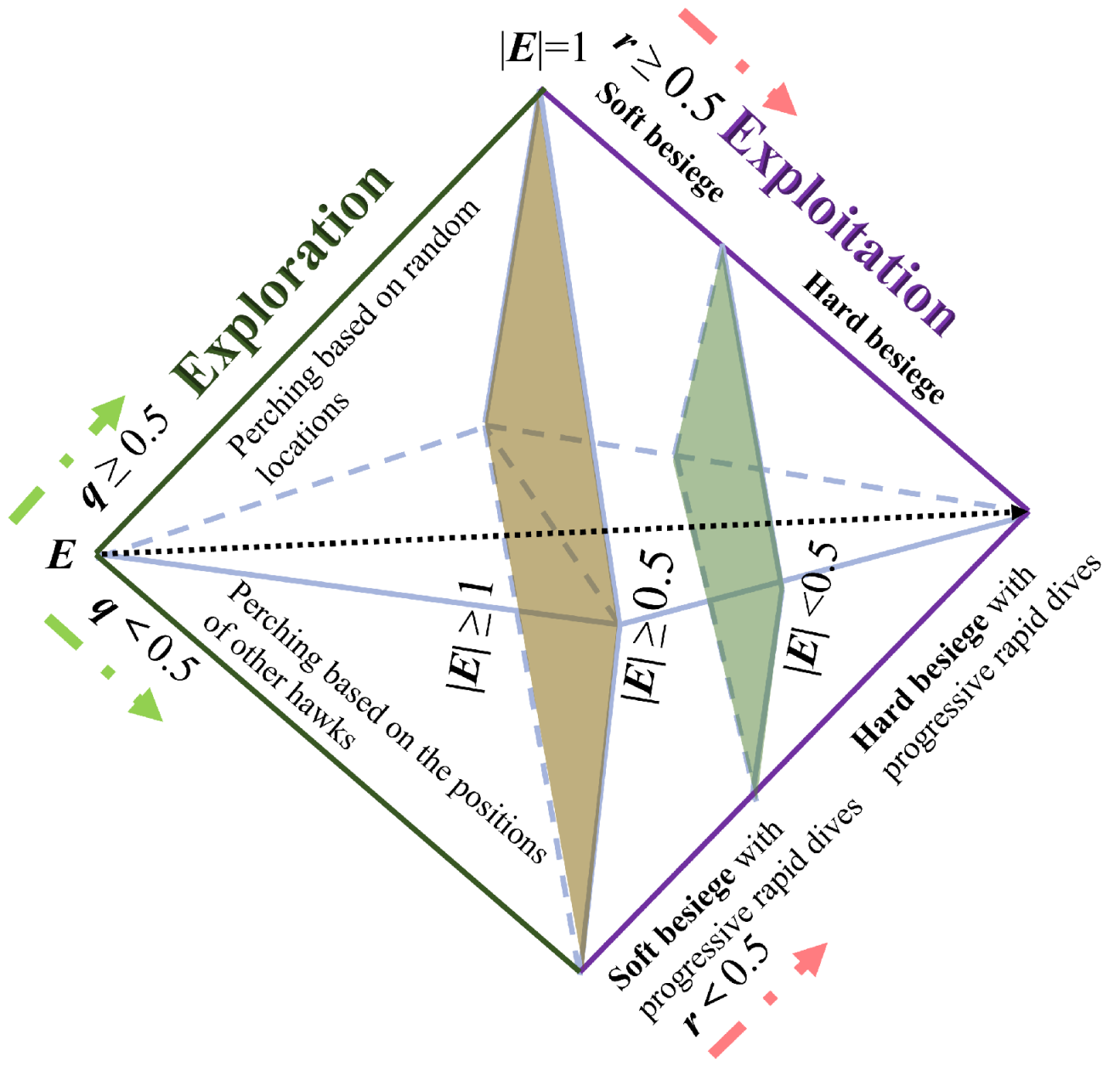
The original HHO algorithm emulates the cooperative behavior and hunting tactics of Harris hawks. Harris hawks initially form an encircling formation around their prey during the capture process. Then, they will employ various types of actions to gradually wear down the prey’s stamina while reducing the distance between themselves and the prey. Finally, when the timing is right, they make a sudden dash to seize the prey. The HHO algorithm employs exploration and exploitation phases to simulate different stages of Harris hawks’ hunting behaviors. Harris hawks will exhibit distinct behavior patterns in different phases. For a specific Harris hawk, it determines the phase it is in according to the prey’s stamina and then performs specific action patterns with a certain probability. Assume that E represents the current stamina of the prey and that q and r are the probabilities of actions. Figure 1 illustrates how the Harris hawk performs different actions based on E, q, and r.
In the original HHO algorithm, the authors defined these actions as continuous operations; thus, it is unable to address FS problems. Zhang et al. [52] in their work transformed the output of the HHO algorithm into binary values (0 or 1) to make it applicable to FS problems. However, this method was too simplistic and rough, which prevented the HHO algorithm from achieving its full potential. On the other hand, Dokeroglu et al. [53] introduced a new set of discrete operations for the HHO algorithm in their work, proposing a novel robust multi-objective HHO algorithm. They applied this algorithm to FS problem and achieved significant results. Building upon the foundation of Dokeroglu’s work, in this paper we introduce a novel set of discrete operations within the framework of the HHO algorithm. Additionally, a feature ranking-based selection mechanism is proposed to further enhance its performance. In the rest parts of this section, we will introduce the details of the proposed BHHO algorithm.

3.2. Proposed BHHO Algorithm

3.2.1. Exploration Phase

As shown in Figure 1, based on the current energy level E of the prey, the entire algorithm is primarily divided into two parts. The energy level of prey (E) decreases during iterations following Equation (1):
E = 2 E 0 ( 1 t T )
where E 0 represents the initial energy, which is randomly assigned a value within the range of [ 1 , 1 ] at the beginning of each iteration. t denotes the current iteration, and T represents the total number of iterations. As the prey gains strength, the initial energy E 0 is adjusted to reflect this by moving towards 1. Conversely, a decrease in E 0 towards 1 signifies the prey is losing stamina. The overall energy level E diminishes as the number of iterations t approaches T, indicating a gradual expenditure of energy.
When the prey has sufficient energy ( | E | 1 ), the algorithm is in the exploration phase. During this phase, it will perform actions based on the probability q, namely either “perching based on random locations” or “perching based on the position of other hawks”. On the other hand, when the prey’s energy is insufficient ( | E | < 1 ), the algorithm enters the exploitation phase. In this phase, depending on the action probability parameter r and the value of the energy level E, it is divided into four different behavioral modes, which including “soft besiege”, “soft besiege with progressive rapid dives”, “hard besiege”, and “hard besiege with progressive rapid dives”.
When the energy level | E | 1 , the proposed BHHO algorithm performs two operations, namely “perching based on random locations” and “perching based on the position of other hawks”. In the first operation, we randomly select a h a w k r from the population, and choose a random number N which is less than the total number of features. Then we swap the positions of the current hawk and h a w k r at N random locations. In the second operation, we randomly select two hawks from the population, namely h a w k 1 and h a w k 2 . Then, we copy the hawk with higher fitness to the individual with lower fitness. Figure 2 shows the example of the two operations. It is noted that in the original HHO, hawks execute only one of the two operations, determined by the factor q. Conversely, in our proposed BHHO, both operations are executed simultaneously during the exploration phase.

3.2.2. Exploitation Phase

When the energy level | E | < 1 , the algorithm is at exploitation. In this phase, according to the action probability parameter r and the value of E. The Harris hawk will take either a soft or hard action based on the prey’s energy level E, while simultaneously seeking an opportunity to capture the prey. When the prey still has sufficient energy left ( | E | > = 0.5 ), the Harris hawk will opt for a soft besiege. In the BHHO algorithm, the soft besiege action will randomly select J positions and copy the values at these positions on the prey to the current Harris hawk. The prey is the best individual among the current population in the BHHO algorithm, and J is a random number that is less than the total number of features. When r < 0.5 , it indicates that the prey has stuck their neck out, and the Harris hawk will attempt to capture the prey directly. The action is called soft besiege with progressive rapid dives in the BHHO algorithm. Specifically, this action select M percent of the positions in the current hawk. The formula for M is as follows:
M = | E | K
where K is the total number of features. Subsequently, values of the selected positions are changed. Figure 3 shows examples of the soft besiege and soft besiege with progressive rapid dives.
Conversely, when the prey’s energy is nearly depleted ( | E | < 0.5 ), the Harris hawk will take hard action. Like the soft action, depending on the value of r, the hard action includes two behavioral patterns: hard besiege ( r > = 0.5 ) and hard besiege with progressive rapid dives ( r < 0.5 ). However, unlike the soft action, we have introduced a new rank-based selection mechanism to further increase the probability of finding superior solutions in the hard action.
The rank-based selection mechanism uses feature rankings to guide the individuals in the BHHO algorithm. Specifically, in “hard besiege” and “hard besiege with progressive rapid dives” we have incorporated two discrete operations. One operation includes the rank-based selection mechanism, while the other operation does not. The two operations generate two new individuals, and the superior one is retained. It should be noted that the ranking of features is derived from filter-based FS methods. Clearly, different filter-based methods will have varying effects in different tasks. To identify a method that is more suitable for addressing the cervical cancer issue, this paper attempts to use three filter-based methods, including the ReliefF (Rf) method [54], the variance thresholding (VT) method [55], and the mutual information (MI) method [56], as tools for feature ranking. The proposed BHHO with these three ranking strategies are referred to as RfBHHO, VTBHHO, and MIBHHO, respectively.
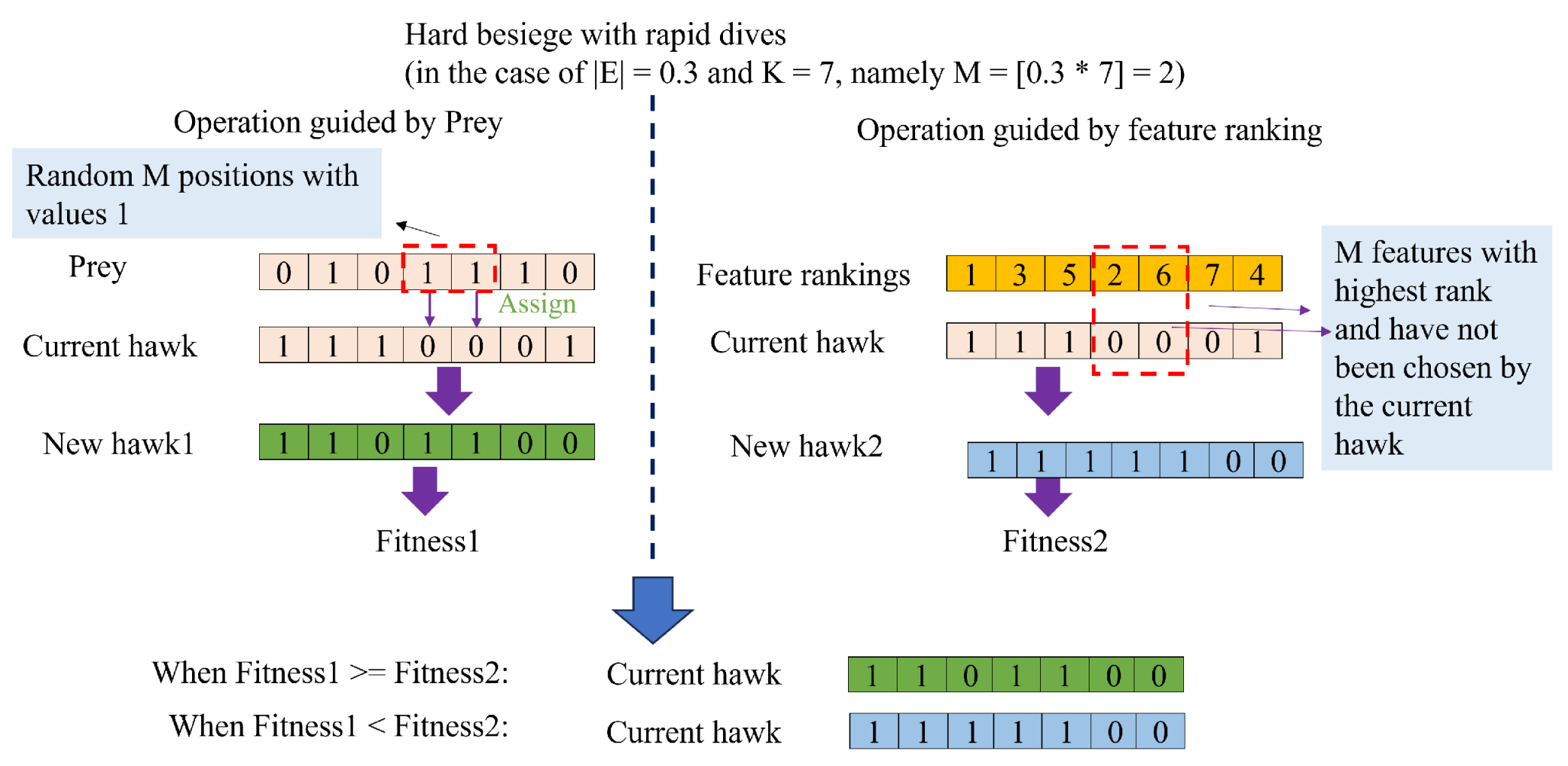
Eventually, the “hard besiege” is defined as follows: First, a position where the value differs between the prey and the current hawk is selected. Then the prey’s value is copied to the current hawk to generate h a w k 1 . Next, we select a feature that has highest rank and has not been chosen by the current hawk, then allow the current hawk select this feature to generate h a w k 2 . Finally, we copy the better one of h a w k 1 and h a w k 2 to the current hawk. For another, the “hard besiege with progressive rapid dives” is defined as follows: First, based on the current prey’s energy, we select M (obtained by Equation (2)) positions with values 1 in the prey, and copy them to the current hawk to generate h a w k 1 . Second, based on the current prey’s energy, we select the top M ranked features that have not yet been chosen by the current hawk, and allow the current hawk select these feature to generate h a w k 2 . Finally, we copy the better one of h a w k 1 and h a w k 2 to the current hawk. We illustrate the examples of hard besiege and hard besiege with progressive rapid dives in Figure 4 and Figure 5, respectively.

3.3. The Theoretical Analysis of the Proposed BHHO Algorithm

As introduced above, we have defined a new set of discrete operators in the BHHO algorithm. Since the E 0 in Equation (1) is a random value, any operation could potentially be executed at any stage of the algorithm. However, due to the presence of the 1 t T term, the prey’s energy level | E | tends to decrease as the algorithm iterates. Therefore, the two operations in the exploration phase are more likely to be executed in the early stages of the algorithm, while the four operations in the exploitation phase are more likely to be executed in the latter half stages.
During the exploration phase, the variable N can be any number from 1 to the total number of features, which offers a larger search space for the individuals. In this part, the algorithm tries to find better optimal solutions through larger step changes. In the exploitation phase, the algorithm introduce the variable M to limit the search space of the individuals. Since the value of M depends on the variable E, the M in soft actions is always larger than in hard actions. During the mid-stages of the algorithm, | E | is more likely to fall into the range of [0.5, 1], indicating that soft actions are more likely to be executed. The individuals can move towards the optimal individual by soft actions, thereby improving the quality of the entire population. At the later stages of the algorithm, | E | is more likely to fall into the range of [0, 0.5], meaning there is a greater possibility of executing hard actions. At this part, since the algorithm has converged or is close to convergence, the algorithm not only utilizes the prey to guide other individuals but also introduces a rank-based selection mechanism to attempt to find better global optimal solutions.
In summary, the entire BHHO algorithm ensures convergence by gradually reducing the search space of the individuals. The specific operation executed by the algorithm is decided by Equation (1), which guarantees the diversity of the population. In addition, the rank-based selection mechanism enhances the algorithm’s capability to search for a global optimal solution. Moreover, there are no other hyper-parameters in the algorithm apart from the population size and the total number of iterations, which greatly alleviates the issue of heuristic algorithms being overly sensitive to hyper-parameters.
The whole process of proposed algorithm is demonstrated in Algorithm 1.
Algorithm 1 Pseudo-code of the proposed BHHO algorithm
  1:
Input: The population size P and the maximum number of iterations T
  2:
Output: Best individual
  3:
Generate the set of feature rankings by a filter-based method
  4:
Calculate the fitness values (F1-score) of hawks
  5:
Designate the optimal hawk as the prey.
  6:
while   t < = T   do
  7:
    i = 1
  8:
    while  i < = P  do
  9:
        Assign a random number from [−1, 1] to E 0
10:
        Calculate the prey’s energy level E
11:
        if  | E | 1  then                        ▹ Exploration phase
12:
           Execute perching based on random locations
13:
           Execute perching based on the position of other hawks
14:
        end if
15:
        if  | E | < 1  then                        ▹ Exploitation phase
16:
           Assign a random number from [0, 1] to r
17:
           if  r > = 0.5 and | E | > = 0.5  then Execute soft besiege
18:
           end if
19:
           if  r > = 0.5 and | E | < 0.5  then Execute hard besiege
20:
           end if
21:
           if  r < 0.5 and | E | > = 0.5  then Execute soft besiege with progressive rapid dives
22:
           end if
23:
           if  r < 0.5 and | E | < 0.5  then Execute hard besiege with progressive rapid dives
24:
           end if
25:
        end if
26:
    end while
27:
    Calculate the fitness values (F1-score) of hawks
28:
    Designate the optimal hawk as the prey.
29:
end while
30:
Output: prey (Best individual)

3.4. Combination of Proposed BHHO and Filter-Based Methods

Wrapper-based FS methods are better at finding feature subset that can improve predication performance, but they also require more computational time. On the other hand, completely useless features in wrapper-based methods may also negatively impact the quality of the final solution. A common hybrid FS strategy to address these issues is to first use filter-based methods to eliminate a small portion of redundant features and then apply wrapper-based methods to process the remaining features. In this paper, we will attempt to combine the best-performing BHHO variant from our experiments with the RF, VT, and MI methods. Specifically, we used the top 90 % ranked features from the Rf, VT, and MI methods separately as the input for the best BHHO variant.

4. Results and Discussion

In this study, seven classifiers include the Support Vector Machine (SVM) [57], the Random Forest (RF) [58], the Naive Bayes (NB) [59], the Adaptive Boosting (Adaboost) [60], the Discriminant Analysis (DA) [61], the Logistic Regression (LR) [62], and the k-Nearest Neighbors (KNN) [63] are used in this paper. In addition, the commonly used wrapper-based methods including GA algorithm, PSO algorithm, and DE algorithm were used for comparison. The flowchart of experiments is illustrated in Figure 6. We commence by preprocessing datasets, which eliminating missing values within datasets. Subsequently, we employ a 5-fold cross-validation scheme to partition the data. In each fold, we conduct an FS operation on the training set. Since the dataset is severely imbalanced, the SMOTE [40] algorithm is used to balancing the training set for a better performance. Then, both the training set and testing set undergo normalization. Finally, we utilize the training set for model training and employ the testing set for performance evaluation. All experiments were conducted on a personal PC with an Intel(R) Core i 9 , 2.20 GHz, and 16 GB memory using Python.

4.1. Dataset

4.1.1. Cervical Cancer Dataset

The cervical cancer dataset is available at the UCI repository and was originally collected from the Hospital Universitario de Caracas in Venezuela. It was utilized in this study. There are 858 records, each characterized by 32 features that encompass habits, sexual history, demographic information, and more. The original dataset includes 55 positive cases and 803 negative cases. Due to privacy concerns, some patients choose not to answer some questions. Hence, the data contains some missing values. Two features, “STDs: Time since first diagnosis” and “STDs: Time since the last diagnosis”, have a total number of 787 missing values. As the number of missing values in the two features exceeds 90 % , we have chosen to remove them. Additionally, there are 105 patients with missing values across 18 features. These patients were excluded from the dataset since more than half of their feature information was incomplete. The rest of the missing values were filled by the Multivariate Imputation by Chained Equation (MICE) method [64]. MICE is a highly flexible imputation method that more accurately measures the uncertainty of missing values compared to other imputation techniques. It replaces missing data by running multiple regression models, where each missing value is imputed based on the other variables in the dataset. To prevent data leakage, we train the MICE algorithm model solely on the training set, and then use the trained model to impute the missing values in the entire dataset. As a result, we have obtained a dataset consisting of information from 753 patients with 30 features. The dataset includes 53 positive cases and 700 negative cases.

4.1.2. Other Datasets

To better illustrate the performance of the proposed BHHO algorithm, we conducted additional experiments on three other disease datasets. These three datasets include the Cleveland dataset [65], the Z-Alizadeh Sani dataset [66], and the Parkinson dataset [67]. The Cleveland dataset contains 303 cases, with 139 positive cases and 164 negative cases. Although this dataset originally comprises 75 features, it is common for most researchers to utilize only 13 of these features. In this study, we also only selected these 13 features as the input to our model. The Z-Alizadeh Sani dataset encompasses 303 cases, consisting of 216 positive cases and 87 negative cases, with a total of 55 features. The Parkinson dataset encompasses 240 cases, consisting of 120 positive cases and 120 negative cases, with a total of 46 features. The objective of both the Cleveland dataset and the Z-Alizadeh Sani dataset is to ascertain whether individuals have heart disease, while the Parkinson dataset aims to identify the presence of Parkinson’s disease in individuals. All three datasets are two classification problems.

4.2. Performance Metrics

In this paper, six metrics including a c c u r a c y , r e c a l l , s p e c i f i c i t y , p r e c i s i o n , F 1 - s c o r e , and G e o m e t r i c - M e a n (G- m e a n ) are employed to evaluate the performance of the proposed method. The equations of these six metrics are defined as follows:
A c c u r a c y = T P + T N T P + F P + T N + F N
R e c a l l = T P T P + E N
S p e c i f i c i t y = T N F P + T N
P r e c i s i o n = T P T P + F P
F 1 s c o r e = 2 R e c a l l P r e c i s i o n R e c a l l + P r e c i s i o n
G m e a n = R e c a l l S p e c i f i c i t y
where T P represents the correct identification of a diseased person as sick; T N signifies the correct classification of a healthy person as being healthy; F P denotes the incorrect classification of a healthy person as diseased; and F N refers to the incorrect classification of a diseased person as healthy. It is noted that the F 1 - s c o r e is used as the objective function when employing wrapper-based methods, with the macro average applied due to the imbalanced nature of the data.

4.3. Validation on the Cervical Cancer Dataset

In this part, we validate the performance of proposed BHHO algorithm on the cervical cancer dataset. Table 1 presents the experimental results without an FS method. The results of proposed BHHO methods are demonstrated in Table 2. In addition, the results of GA method, PSO method, and DE method are shown in Table 3. Since we employed a 5-fold strategy to partition the dataset, all the table presents the experimental results in the form of “mean ± variance”.
Clearly, all the experimental results exhibit high a c c u r a c y and p r e c i s i o n but low s e n s i t i v i t y and s p e c i f i c i t y . This is because the dataset belongs to the category of highly imbalanced datasets, namely, the majority class vastly outnumbers the minority class. In the real world, the diagnosis of cervical cancer is precisely such a situation where negative results overwhelmingly outnumber positive results. In such a situation, using simple metrics like a c c u r a c y or p r e c i s i o n may not accurately assess the performance since these two metrics can easily yield high value when the majority class greatly outnumbers the minority class. In the case of cervical cancer, the consequences of incorrectly predicting the minority class are much more severe than incorrectly predicting the majority class. Therefore, we pay more attention to the results of r e c a l l and s p e c i f i c i t y . However, this does not mean that a c c u r a c y and p r e c i s i o n should be ignored. To comprehensively evaluate the performance, F1-score and G-mean are used as the main reference indicators in our experiments. So, we have highlighted the best F1-score and G-mean in bold on each table.
From the three tables, it can be observed that when using the wrapper-based methods, most results tend to be better than those obtained using all features, which represents that using wrapper-based FS algorithms can capturing the implicit relationships between features, effectively reducing the number of features while improving performance. From Table 2, it can be observed that among three BHHO variants, VTBHHO achieved the highest F1-score of 28.60 when using Adaboost as the classifier and the highest G-mean of 64.18 when using LR as the classifier. Furthermore, it can be found that the highest result obtained by proposed BHHO algorithm surpasses all outcomes using the GA method, PSO method, and DE method. Figure 7 visually demonstrated such a situation. In Figure 7, the best F1-score and G-mean of each wrapper-based method are selected as representatives. The specific values and the classifiers that achieved these results are annotated above each bar. Clearly, the best results from all the wrapper-based methods surpassed the best results obtained using all features, and the best results from proposed BHHO methods surpassed other commonly used wrapper-based methods.
Table 4, Table 5, Table 6 show the experimental results after employing Rf method, VT method, and MI method. The top 50 % , 60 % , 70 % , and 80 % of features are selected as the features subset. It can be observed that when using Rf method, most classifiers did not surpass the performance of the original feature set, while when using VT method or MI method, a majority of the classifiers managed to exceed the performance of the original feature set, while there were still some classifiers that experienced a decline in performance. It is worth emphasizing that only in MI method (using top 80 % of features), the performance of DA completely surpassed the results of all classifiers using the all feature set. But this result is still less than majority of wrapper-based method. It is evident that not all FS methods yield positive results. While filter-based FS methods can reduce redundant features and enhance accuracy to some extent, their effectiveness is quite limited. In some cases, this method may even degrade the performance. This is because the importance of features in a dataset cannot be judged solely from a statistical perspective. The relationships between features must also be considered. Some features, which might seem statistically insignificant on their own, can significantly improve performance when used in conjunction with other features. Filter-based methods often overlook this aspect. Therefore, in practical applications, most researchers do not rely solely on filter-based methods.
Based on the above validation, we further attempted a hybrid method that first uses filter-based methods to eliminate a small portion of redundant features and then applies proposed BHHO methods to process the remaining features. Specifically, we used the top 90 % ranked features from the Rf, VT, and MI methods separately as the input for the VTBHHO method. The results of the experiment are shown in Table 7. We bold the best F1-score and G-mean among all results. In the combination of Rf and VTBHHO, the highest F1-score ( 30.21 % ) was obtained when using SVM as the classifier. In the combination of MI and VTBHHO, the highest G-mean ( 61.69 % ) was achieved when using Adaboost as the classifier. It can be observed that, compared to using VTBHHO alone, the hybrid approaches achieved a higher F1-score but obtained a lower G-mean. This is because we used the F1-score as the objective function for the wrapped-based methods, so the methods are more inclined to favor feature subsets that can improve the F1-score. When using wrapper-based methods alone, some features with negative effects impacted the quality of the final solution. However, by first using filter-based methods to eliminate those features that were most likely completely useless, the quality of all feature subsets was improved, thereby increasing the likelihood of obtaining better solutions.
Finally, we analyze the selected feature sets obtained when combining Rf and VTBHHO (using SVM as the classifier), that is, the situation that achieves the highest F1-score. The selected feature results are shown in Table 8. Obviously, when the distribution of the dataset varies, even using the same FS method and classifier, the selected features can vary significantly. In the five different subsets of the dataset, the number of features used ranged from a maximum of 18 features to a minimum of 8 features among the 30 features. The table summarizes the usage of all features, and it can be observed that the last feature “DX” has been used in all subsets. This suggests that past diagnostic results play a crucial role in the current decision-making process. Additionally, “Hormonal Contraceptives (year)”, “STDs”, “STDs:syphilis”, and “STDs:molluscum contagiosum” have been used four times, indicating that these risk factors significantly increase the likelihood of cervical cancer detection. On the other hand, “STDs:condylomatosis” and “STDs:cervical condylomatosis” have been shown to have no association with the discovery of cervical cancer. These statistical findings can provide valuable recommendations to the general population. When highly relevant risk factors appear in daily life, we should be vigilant and seek further medical diagnosis.

4.4. Validation on Other Datasets

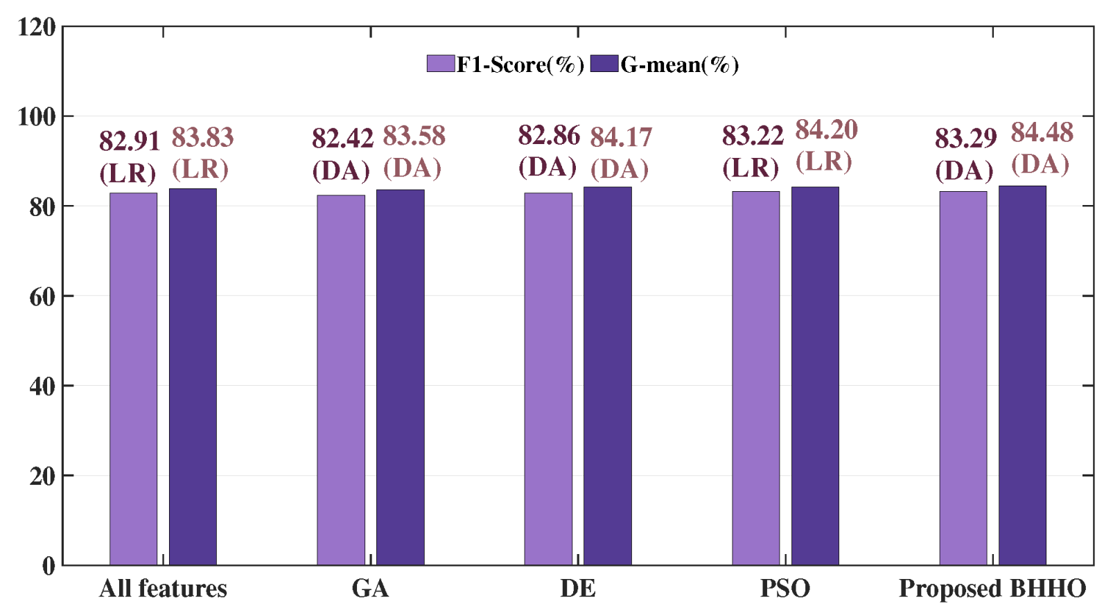
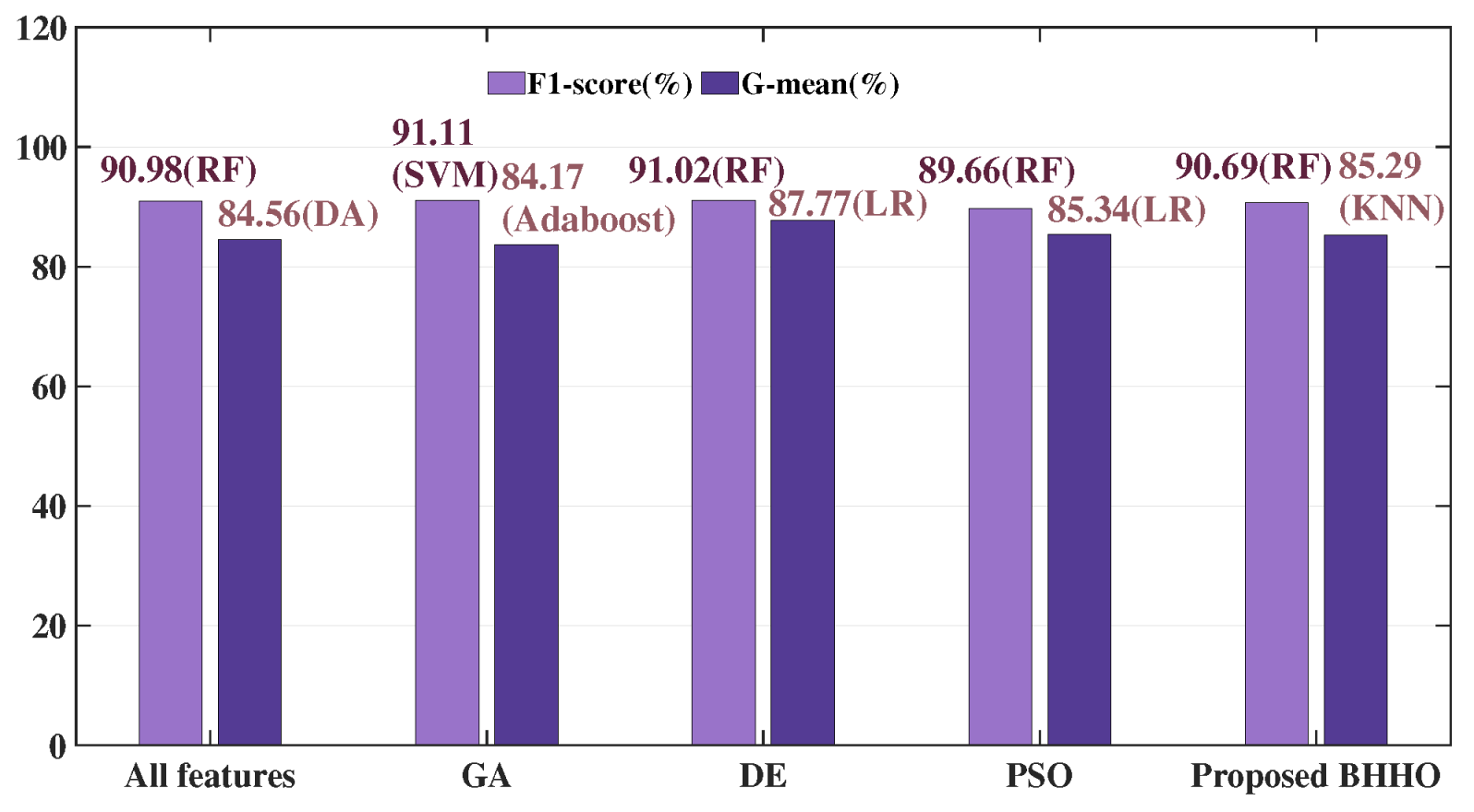
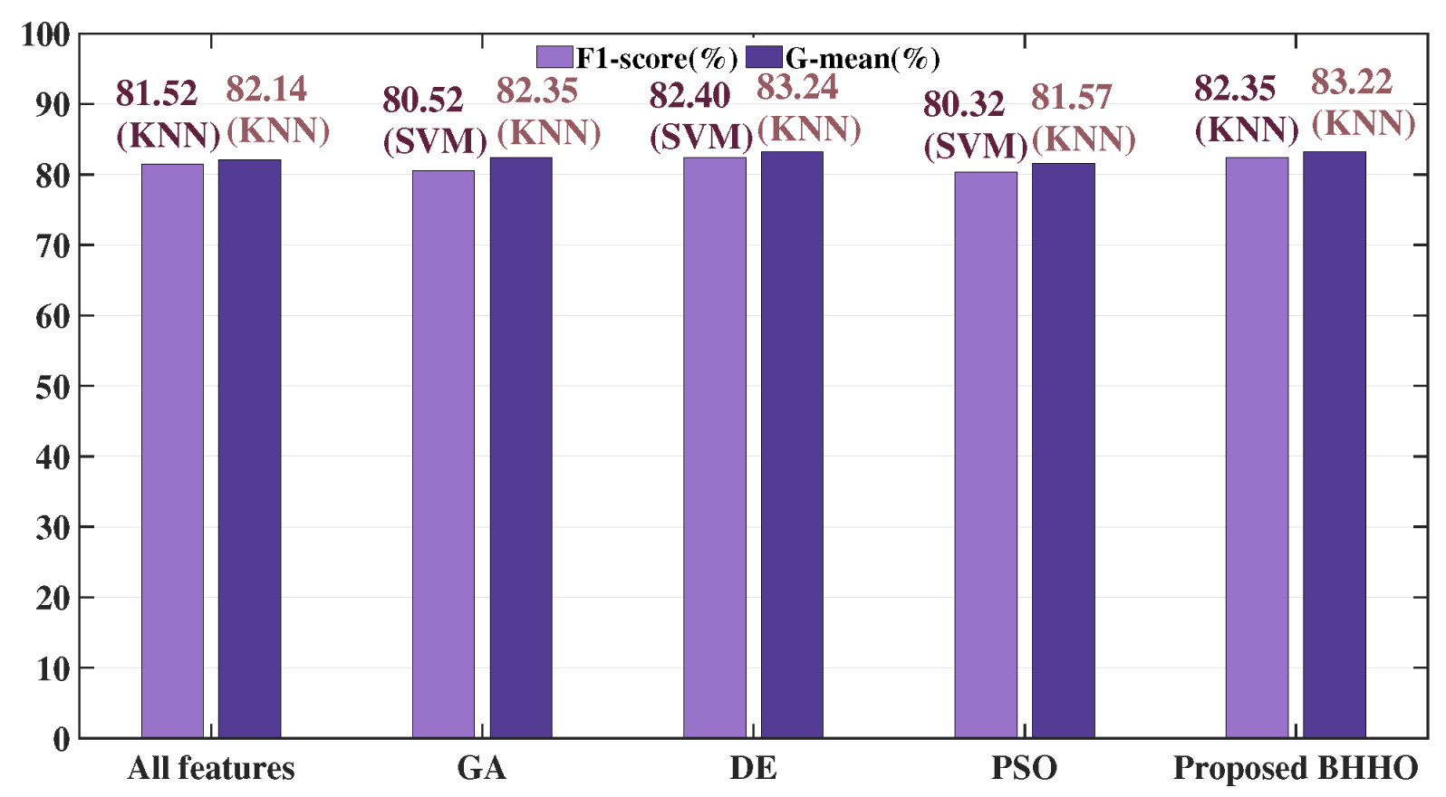
In this part, we validate the proposed BHHO algorithm on the other three disease datasets. The experimental results are shown in Table 9, Table 10, Table 11, Table 12, Table 13 and Table 14 that are presented in the form of m e a n ± v a r i a n c e , and the best F1-score and G-mean of each method are highlighted in bold. On the Cleveland dataset, VTBHHO’s DA achieved the best F1-score ( 83.29 % ) and G-mean ( 84.2 % ). On the Z-Alizadeh Sani dataset, GA’s SVM achieved the highest F1-score ( 91.11 % ), while DE’s LR obtained the highest G-mean ( 87.77 % ). On the Parkinson’s dataset, MIBHHO’s KNN achieved the best F1-score ( 82.35 % ) and the highest G-mean ( 83.22 % ). Figure 8, Figure 9 and Figure 10 illustrate the experimental conditions for these three datasets using barcharts. The proposed BHHO achieved the best results in two out of the three datasets. Although it did not achieve the best result on the Z-Alizadeh Sani dataset, it still performed close to the optimal outcome. It demonstrates that the proposed BHHO method is not only effective for cervical cancer dataset but also has a certain degree of generalizability to other disease datasets. Furthermore, observing the results of the three BHHO variants on different datasets reveals that different ranking strategies play varying roles depending on the dataset. The VTBHHHO variant, which performed best on the cervical cancer dataset, may not necessarily be the optimal choice for other datasets. Therefore, we can adjust the ranking strategy according to the actual tasks to achieve higher performance. In other words, the ranking strategy incorporated into BHHO allows it to flexibly adapt to different environments. Although the combination of the proposed BHHO with RF, VT, and MI did not achieve the best results on the Z-Alizadeh Sani dataset, it can be expected that combining it with other ranking strategies could yield higher accuracy. In summary, the experimental results prove that proposed BHHO method can offer a competitive performance than other commonly used methods.
5. Conclusions

This study introduces a novel feature selection (FS) strategy for the automated diagnosis of cervical cancer using machine learning (ML). Disease datasets typically contain a large number of features, but a lot of them are redundant or irrelevant. Utilizing wrapper-based FS methods to eliminate these useless features is currently one of the effective methods for this problem. Following this perspective, in this paper, we have improved the Harris Hawks Optimization (HHO) algorithm to propose the Binary Harris Hawks Optimization (BHHO) algorithm. Specifically, we have defined a new set of discrete operations under the framework of HHO to better address the FS problem. Additionally, we introduced a new rank-based selection mechanism into the algorithm to enhance its optimization ability.
To comprehensively evaluate the performance of the proposed algorithms, we compared the proposed BHHO algorithm with commonly used wrapper-based and filter-based FS methods. The results shows that the proposed BHHO algorithm achieves better results on the cervical cancer problem than other commonly used methods. In addition, we attempted a hybrid approach by combining the filter-based method and the BHHO algorithm. As a result, the hybrid approach achieved the highest F1-score among all experiments. Moreover, the proposed BHHO algorithm was validated on other disease datasets. Experimental results shows the BHHO algorithm can provide competitive performance even on other datasets, which proves its generalizability. In future work, we plan to explore the integration of other feature ranking methods and the proposed BHHO algorithm. Additionally, we will explore using alternative functions such as G-mean or aggregate function as the algorithm’s objective function.

Author Contributions

Conceptualization, M.D.; Software, M.D.; Validation, Y.W. and Y.H.; Formal analysis, Y.W. and Y.H.; Data curation, Y.H.; Writing—original draft, M.D.; Supervision, Y.T. All authors have read and agreed to the published version of the manuscript.

Funding

This research was funded by JST SPRING grant number JPMJSP2135. The APC was funded by JST SPRING.

Data Availability Statement

Conflicts of Interest

The authors declare no conflicts of interest.

References

  1. Sung, H.; Ferlay, J.; Siegel, R.L.; Laversanne, M.; Soerjomataram, I.; Jemal, A.; Bray, F. Global cancer statistics 2020: GLOBOCAN estimates of incidence and mortality worldwide for 36 cancers in 185 countries. CA Cancer J. Clin. 2021, 71, 209–249. [Google Scholar] [CrossRef]
  2. Gadducci, A.; Barsotti, C.; Cosio, S.; Domenici, L.; Riccardo Genazzani, A. Smoking habit, immune suppression, oral contraceptive use, and hormone replacement therapy use and cervical carcinogenesis: A review of the literature. Gynecol. Endocrinol. 2011, 27, 597–604. [Google Scholar] [CrossRef]
  3. Rodríguez, A.C.; Schiffman, M.; Herrero, R.; Hildesheim, A.; Bratti, C.; Sherman, M.E.; Solomon, D.; Guillén, D.; Alfaro, M.; Morales, J.; et al. Longitudinal study of human papillomavirus persistence and cervical intraepithelial neoplasia grade 2/3: Critical role of duration of infection. J. Natl. Cancer Inst. 2010, 102, 315–324. [Google Scholar] [CrossRef]
  4. Hillemanns, P.; Soergel, P.; Hertel, H.; Jentschke, M. Epidemiology and early detection of cervical cancer. Oncol. Res. Treat. 2016, 39, 501–506. [Google Scholar] [CrossRef]
  5. World Health Organization. Comprehensive Cervical Cancer Control: A Guide to Essential Practice; World Health Organization: Geneva, Switzerland, 2006.
  6. Bray, F.; Ferlay, J.; Soerjomataram, I.; Siegel, R.L.; Torre, L.A.; Jemal, A. Global cancer statistics 2018: GLOBOCAN estimates of incidence and mortality worldwide for 36 cancers in 185 countries. CA Cancer J. Clin. 2018, 68, 394–424. [Google Scholar] [CrossRef]
  7. Firmino, M.; Angelo, G.; Morais, H.; Dantas, M.R.; Valentim, R. Computer-aided detection (CADe) and diagnosis (CADx) system for lung cancer with likelihood of malignancy. Biomed. Eng. Online 2016, 15, 2. [Google Scholar] [CrossRef]
  8. Setio, A.A.A.; Ciompi, F.; Litjens, G.; Gerke, P.; Jacobs, C.; Van Riel, S.J.; Wille, M.M.W.; Naqibullah, M.; Sánchez, C.I.; Van Ginneken, B. Pulmonary nodule detection in CT images: False positive reduction using multi-view convolutional networks. IEEE Trans. Med. Imaging 2016, 35, 1160–1169. [Google Scholar] [CrossRef]
  9. Abdel-Zaher, A.M.; Eldeib, A.M. Breast cancer classification using deep belief networks. Expert Syst. Appl. 2016, 46, 139–144. [Google Scholar] [CrossRef]
  10. Mughal, B.; Sharif, M.; Muhammad, N.; Saba, T. A novel classification scheme to decline the mortality rate among women due to breast tumor. Microsc. Res. Tech. 2018, 81, 171–180. [Google Scholar] [CrossRef]
  11. Ben-Cohen, A.; Diamant, I.; Klang, E.; Amitai, M.; Greenspan, H. Fully convolutional network for liver segmentation and lesions detection. In Proceedings of the Deep Learning and Data Labeling for Medical Applications: First International Workshop, LABELS 2016, and Second International Workshop, DLMIA 2016, Held in Conjunction with MICCAI 2016, Athens, Greece, 21 October 2016; Proceedings 1. Springer: Cham, Switzerland, 2016; pp. 77–85. [Google Scholar]
  12. Rau, H.H.; Hsu, C.Y.; Lin, Y.A.; Atique, S.; Fuad, A.; Wei, L.M.; Hsu, M.H. Development of a web-based liver cancer prediction model for type II diabetes patients by using an artificial neural network. Comput. Methods Programs Biomed. 2016, 125, 58–65. [Google Scholar] [CrossRef]
  13. Asuntha, A.; Srinivasan, A. Deep learning for lung Cancer detection and classification. Multimed. Tools Appl. 2020, 79, 7731–7762. [Google Scholar] [CrossRef]
  14. Shanthi, S.; Rajkumar, N. Lung cancer prediction using stochastic diffusion search (SDS) based feature selection and machine learning methods. Neural Process. Lett. 2021, 53, 2617–2630. [Google Scholar] [CrossRef]
  15. Acharya, S.; Alsadoon, A.; Prasad, P.; Abdullah, S.; Deva, A. Deep convolutional network for breast cancer classification: Enhanced loss function (ELF). J. Supercomput. 2020, 76, 8548–8565. [Google Scholar] [CrossRef]
  16. Ak, M.F. A comparative analysis of breast cancer detection and diagnosis using data visualization and machine learning applications. Healthcare 2020, 8, 111. [Google Scholar] [CrossRef]
  17. Saba, L.; Dey, N.; Ashour, A.S.; Samanta, S.; Nath, S.S.; Chakraborty, S.; Sanches, J.; Kumar, D.; Marinho, R.; Suri, J.S. Automated stratification of liver disease in ultrasound: An online accurate feature classification paradigm. Comput. Methods Programs Biomed. 2016, 130, 118–134. [Google Scholar] [CrossRef]
  18. Gatos, I.; Tsantis, S.; Spiliopoulos, S.; Karnabatidis, D.; Theotokas, I.; Zoumpoulis, P.; Loupas, T.; Hazle, J.D.; Kagadis, G.C. A machine-learning algorithm toward color analysis for chronic liver disease classification, employing ultrasound shear wave elastography. Ultrasound Med. Biol. 2017, 43, 1797–1810. [Google Scholar] [CrossRef]
  19. Bellman, R. Dynamic programming. Science 1966, 153, 34–37. [Google Scholar] [CrossRef]
  20. Manikandan, G.; Abirami, S. A survey on feature selection and extraction techniques for high-dimensional microarray datasets. In Knowledge Computing and its Applications: Knowledge Computing in Specific Domains: Volume II; Springer: Singapore, 2018; pp. 311–333. [Google Scholar]
  21. William, W.; Ware, A.; Basaza-Ejiri, A.H.; Obungoloch, J. A review of image analysis and machine learning techniques for automated cervical cancer screening from pap-smear images. Comput. Methods Programs Biomed. 2018, 164, 15–22. [Google Scholar] [CrossRef]
  22. Liu, W.; Li, C.; Xu, N.; Jiang, T.; Rahaman, M.M.; Sun, H.; Wu, X.; Hu, W.; Chen, H.; Sun, C.; et al. CVM-Cervix: A hybrid cervical Pap-smear image classification framework using CNN, visual transformer and multilayer perceptron. Pattern Recognit. 2022, 130, 108829. [Google Scholar] [CrossRef]
  23. Dosovitskiy, A.; Beyer, L.; Kolesnikov, A.; Weissenborn, D.; Zhai, X.; Unterthiner, T.; Dehghani, M.; Minderer, M.; Heigold, G.; Gelly, S.; et al. An image is worth 16x16 words: Transformers for image recognition at scale. arXiv 2020, arXiv:2010.11929. [Google Scholar]
  24. Touvron, H.; Cord, M.; Douze, M.; Massa, F.; Sablayrolles, A.; Jégou, H. Training data-efficient image transformers & distillation through attention. In Proceedings of the International Conference on Machine Learning (PMLR), Virtual, 18–24 July 2021; pp. 10347–10357. [Google Scholar]
  25. Pramanik, R.; Biswas, M.; Sen, S.; de Souza Júnior, L.A.; Papa, J.P.; Sarkar, R. A fuzzy distance-based ensemble of deep models for cervical cancer detection. Comput. Methods Programs Biomed. 2022, 219, 106776. [Google Scholar] [CrossRef]
  26. Szegedy, C.; Vanhoucke, V.; Ioffe, S.; Shlens, J.; Wojna, Z. Rethinking the inception architecture for computer vision. In Proceedings of the IEEE Conference on Computer Vision and Pattern Recognition, Las Vegas, NV, USA, 27–30 June 2016; pp. 2818–2826. [Google Scholar]
  27. Sandler, M.; Howard, A.; Zhu, M.; Zhmoginov, A.; Chen, L.C. Mobilenetv2: Inverted residuals and linear bottlenecks. In Proceedings of the IEEE Conference on Computer Vision and Pattern Recognition, Salt Lake City, UT, USA, 18–23 June 2018; pp. 4510–4520. [Google Scholar]
  28. He, K.; Zhang, X.; Ren, S.; Sun, J. Deep residual learning for image recognition. In Proceedings of the IEEE Conference on Computer Vision and Pattern Recognition, Las Vegas, NV, USA, 27–30 June 2016; pp. 770–778. [Google Scholar]
  29. Yaman, O.; Tuncer, T. Exemplar pyramid deep feature extraction based cervical cancer image classification model using pap-smear images. Biomed. Signal Process. Control 2022, 73, 103428. [Google Scholar] [CrossRef]
  30. Shi, J.; Wang, R.; Zheng, Y.; Jiang, Z.; Zhang, H.; Yu, L. Cervical cell classification with graph convolutional network. Comput. Methods Programs Biomed. 2021, 198, 105807. [Google Scholar] [CrossRef]
  31. Tripathi, A.; Arora, A.; Bhan, A. Classification of cervical cancer using Deep Learning Algorithm. In Proceedings of the 2021 5th International Conference on Intelligent Computing and Control Systems (ICICCS), Madurai, India, 6–8 May 2021; pp. 1210–1218. [Google Scholar]
  32. Cancer Genome Atlas Research Network. Integrated genomic and molecular characterization of cervical cancer. Nature 2017, 543, 378. [Google Scholar] [CrossRef]
  33. Nahand, J.S.; Taghizadeh-boroujeni, S.; Karimzadeh, M.; Borran, S.; Pourhanifeh, M.H.; Moghoofei, M.; Bokharaei-Salim, F.; Karampoor, S.; Jafari, A.; Asemi, Z.; et al. microRNAs: New prognostic, diagnostic, and therapeutic biomarkers in cervical cancer. J. Cell. Physiol. 2019, 234, 17064–17099. [Google Scholar] [CrossRef]
  34. Luo, W.; Wang, M.; Liu, J.; Cui, X.; Wang, H. Identification of a six lncRNAs signature as novel diagnostic biomarkers for cervical cancer. J. Cell. Physiol. 2020, 235, 993–1000. [Google Scholar] [CrossRef]
  35. Bock, C. Analysing and interpreting DNA methylation data. Nat. Rev. Genet. 2012, 13, 705–719. [Google Scholar] [CrossRef]
  36. Qureshi, S.A.; Bashir, M.U.; Yaqinuddin, A. Utility of DNA methylation markers for diagnosing cancer. Int. J. Surg. 2010, 8, 194–198. [Google Scholar] [CrossRef]
  37. Xu, W.; Xu, M.; Wang, L.; Zhou, W.; Xiang, R.; Shi, Y.; Zhang, Y.; Piao, Y. Integrative analysis of DNA methylation and gene expression identified cervical cancer-specific diagnostic biomarkers. Signal Transduct. Target. Ther. 2019, 4, 55. [Google Scholar] [CrossRef]
  38. Dua, D.; Graff, C. UCI Machine Learning Repository. 2017. Available online: http://archive.ics.uci.edu/ml (accessed on 1 February 2024).
  39. Newaz, A.; Muhtadi, S.; Haq, F.S. An intelligent decision support system for the accurate diagnosis of cervical cancer. Knowl.-Based Syst. 2022, 245, 108634. [Google Scholar] [CrossRef]
  40. Chawla, N.V.; Bowyer, K.W.; Hall, L.O.; Kegelmeyer, W.P. SMOTE: Synthetic minority over-sampling technique. J. Artif. Intell. Res. 2002, 16, 321–357. [Google Scholar] [CrossRef]
  41. Hart, P. The condensed nearest neighbor rule (corresp.). IEEE Trans. Inf. Theory 1968, 14, 515–516. [Google Scholar] [CrossRef]
  42. Wilson, D.L. Asymptotic properties of nearest neighbor rules using edited data. IEEE Trans. Syst. Man Cybern. 1972; SMC-2, 408–421. [Google Scholar]
  43. Lu, J.; Song, E.; Ghoneim, A.; Alrashoud, M. Machine learning for assisting cervical cancer diagnosis: An ensemble approach. Future Gener. Comput. Syst. 2020, 106, 199–205. [Google Scholar] [CrossRef]
  44. Bolón-Canedo, V.; Sánchez-Maroño, N.; Alonso-Betanzos, A. Distributed feature selection: An application to microarray data classification. Appl. Soft Comput. 2015, 30, 136–150. [Google Scholar] [CrossRef]
  45. Saw, T.; Myint, P.H. Swarm intelligence based feature selection for high dimensional classification: A literature survey. Int. J. Comput 2019, 33, 69–83. [Google Scholar]
  46. Alhenawi, E.; Al-Sayyed, R.; Hudaib, A.; Mirjalili, S. Feature selection methods on gene expression microarray data for cancer classification: A systematic review. Comput. Biol. Med. 2022, 140, 105051. [Google Scholar] [CrossRef] [PubMed]
  47. Nithya, B.; Ilango, V. Evaluation of machine learning based optimized feature selection approaches and classification methods for cervical cancer prediction. SN Appl. Sci. 2019, 1, 641. [Google Scholar] [CrossRef]
  48. Holland, J.H. Adaptation in Natural and Artificial Systems: An Introductory Analysis with Applications to Biology, Control, and Artificial Intelligence; MIT Press: Cambridge, MA, USA, 1992. [Google Scholar]
  49. Storn, R.; Price, K. Differential evolution—A simple and efficient heuristic for global optimization over continuous spaces. J. Glob. Optim. 1997, 11, 341–359. [Google Scholar] [CrossRef]
  50. Kennedy, J.; Eberhart, R. Particle swarm optimization. In Proceedings of the ICNN’95-International Conference on Neural Networks, Perth, WA, Australia, 27 November–1 December 1995; Volume 4, pp. 1942–1948. [Google Scholar]
  51. Heidari, A.A.; Mirjalili, S.; Faris, H.; Aljarah, I.; Mafarja, M.; Chen, H. Harris hawks optimization: Algorithm and applications. Future Gener. Comput. Syst. 2019, 97, 849–872. [Google Scholar] [CrossRef]
  52. Zhang, Y.; Liu, R.; Wang, X.; Chen, H.; Li, C. Boosted binary Harris hawks optimizer and feature selection. Eng. Comput. 2021, 37, 3741–3770. [Google Scholar] [CrossRef]
  53. Dokeroglu, T.; Deniz, A.; Kiziloz, H.E. A robust multiobjective Harris’ Hawks Optimization algorithm for the binary classification problem. Knowl.-Based Syst. 2021, 227, 107219. [Google Scholar] [CrossRef]
  54. Kira, K.; Rendell, L.A. The feature selection problem: Traditional methods and a new algorithm. In Proceedings of the Tenth National Conference on Artificial Intelligence, San Jose, CA, USA, 12–16 July 1992; pp. 129–134. [Google Scholar]
  55. Guyon, I.; Weston, J.; Barnhill, S.; Vapnik, V. Gene selection for cancer classification using support vector machines. Mach. Learn. 2002, 46, 389–422. [Google Scholar] [CrossRef]
  56. Peng, H.; Long, F.; Ding, C. Feature selection based on mutual information criteria of max-dependency, max-relevance, and min-redundancy. IEEE Trans. Pattern Anal. Mach. Intell. 2005, 27, 1226–1238. [Google Scholar] [CrossRef]
  57. Cortes, C.; Vapnik, V. Support-vector networks. Mach. Learn. 1995, 20, 273–297. [Google Scholar] [CrossRef]
  58. Breiman, L. Random forests. Mach. Learn. 2001, 45, 5–32. [Google Scholar] [CrossRef]
  59. Sahami, M.; Dumais, S.; Heckerman, D.; Horvitz, E. A Bayesian approach to filtering junk e-mail. In Proceedings of the Learning for Text Categorization: Papers from the 1998 Workshop, Madison, WI, USA, 26–27 July 1998; Volume 62, pp. 98–105. [Google Scholar]
  60. Freund, Y.; Schapire, R.E. A decision-theoretic generalization of on-line learning and an application to boosting. J. Comput. Syst. Sci. 1997, 55, 119–139. [Google Scholar] [CrossRef]
  61. Fisher, R.A. The use of multiple measurements in taxonomic problems. Ann. Eugen. 1936, 7, 179–188. [Google Scholar] [CrossRef]
  62. Cox, D.R.; Snell, E.J. Analysis of Binary Data; CRC Press: Boca Raton, FL, USA, 1989; Volume 32. [Google Scholar]
  63. Cover, T.; Hart, P. Nearest neighbor pattern classification. IEEE Trans. Inf. Theory 1967, 13, 21–27. [Google Scholar] [CrossRef]
  64. Van Buuren S, Oudshoorn C G M Multivariate imputation by chained equations. J. Stat. Softw. 2011, 45, 1–67.
  65. Janosi, A.; Steinbrunn, W.; Pfisterer, M.; Detrano, R. Heart Disease; UCI Machine Learning Repository: Espoo, Finland, 1988. [Google Scholar] [CrossRef]
  66. Alizadehsani, R.; Roshanzamir, M.; Sani, Z. Z-Alizadeh Sani; UCI Machine Learning Repository: Espoo, Finland, 2017. [Google Scholar] [CrossRef]
  67. Prez, C. Parkinson Dataset with Replicated Acoustic Features; UCI Machine Learning Repository: Espoo, Finland, 2019. [Google Scholar] [CrossRef]
Figure 1. The schematic diagram of the HHO algorithm.
Electronics 13 02554 g001
Figure 2. The examples of operations in the exploration phase.
Electronics 13 02554 g002
Figure 3. The examples of operations of soft actions.
Electronics 13 02554 g003
Figure 4. The examples of hard besiege.
Electronics 13 02554 g004
Figure 5. The examples of hard besiege with rapid dives.
Electronics 13 02554 g005
Figure 6. Flowchart of the experimental framework.
Electronics 13 02554 g006
Figure 7. Bar chart for the results of the cervical cancer dataset. Each bar denotes the best result under the feature selection method. There is a specific numerical value along with the classifier’s name at the top of each bar.
Electronics 13 02554 g007
Figure 8. Bar chart for the results of the Cleveland dataset. Each bar denotes the best result under the feature selection method. There is a specific numerical value along with the classifier’s name at the top of each bar.
Electronics 13 02554 g008
Figure 9. Bar chart for the results of the Z-Alizadeh Sani dataset. Each bar denotes the best result under the feature selection method. There is a specific numerical value along with the classifier’s name at the top of each bar.
Electronics 13 02554 g009
Figure 10. Bar chart for the results of the Parkinson dataset. Each bar denotes the best result under the feature selection method. There is a specific numerical value along with the classifier’s name at the top of each bar.
Electronics 13 02554 g010
Table 1. Results for cervical cancer dataset with all features. The best F1-score and G-mean across all methods are highlighted in bold.
ClassifierAccuracy (%)Sensitivity (%)Specificity (%)Precision (%)F1-Score (%)G-Mean (%)
SVM87.25 ± 1.4020.42 ± 5.3019.05 ± 10.1692.33 ± 2.6118.59 ± 6.0543.06 ± 5.33
RF90.97 ± 1.559.14 ± 10.4815.67 ± 13.4897.29 ± 0.9110.52 ± 10.0622.01 ± 19.97
NB78.21 ± 7.5129.40 ± 20.0112.00 ± 5.8381.85 ± 9.3314.74 ± 6.5945.17 ± 14.28
Adaboost80.08 ± 1.4831.77 ± 7.7413.06 ± 4.7083.73 ± 2.0218.25 ± 5.7651.12 ± 6.70
DA83.66 ± 1.0941.87 ± 13.4519.28 ± 7.0986.88 ± 1.6625.90 ± 8.6159.34 ± 10.55
LR80.61 ± 0.5534.62 ± 8.6213.92 ± 3.9484.16 ± 0.9919.56 ± 4.7553.44 ± 7.28
KNN78.22 ± 1.0043.90 ± 7.9315.02 ± 4.7980.72 ± 0.8922.26 ± 6.3759.26 ± 5.96
Table 2. Results for cervical cancer dataset using proposed BHHO variants. The best F1-score and G-mean across all methods are highlighted in bold.
VTBHHO
ClassifierAccuracy (%)Sensitivity (%)Specificity (%)Precision (%)F1-score (%)G-mean (%)
SVM87.78 ± 1.4631.77 ± 10.0322.88 ± 5.5792.15 ± 1.5825.82 ± 5.8453.33 ± 8.77
RF89.11 ± 1.7311.35 ± 2.4218.87 ± 12.1895.03 ± 2.5912.97 ± 4.3932.65 ± 3.42
NB76.89 ± 8.1535.58 ± 17.4511.82 ± 3.7080.19 ± 10.2816.35 ± 4.1550.35 ± 12.35
Adaboost83.67 ± 2.2646.96 ± 8.5120.78 ± 4.6986.42 ± 2.0928.60 ± 5.9263.46 ± 5.48
DA84.99 ± 3.3232.23 ± 12.5217.75 ± 6.4588.96 ± 2.7322.85 ± 8.5052.08 ± 12.43
LR81.68 ± 1.9549.53 ± 10.5919.04 ± 4.5684.15 ± 1.9127.21 ± 5.9664.18 ± 6.81
KNN83.13 ± 2.6021.66 ± 13.8911.39 ± 6.8487.53 ± 2.7614.89 ± 9.1338.10 ± 20.26
RfBHHO
ClassifierAccuracy (%)Sensitivity (%)Specificity (%)Precision (%)F1-score (%)G-mean (%)
SVM86.85 ± 1.9828.13 ± 12.3818.90 ± 6.4791.44 ± 2.0021.92 ± 7.6449.18 ± 12.12
RF87.64 ± 2.7713.74 ± 4.9916.21 ± 12.0793.29 ± 2.7913.85 ± 6.7735.17 ± 6.83
NB80.47 ± 7.4630.73 ± 15.5712.78 ± 3.7484.27 ± 9.0817.00 ± 4.7048.30 ± 11.31
Adaboost83.54 ± 3.1738.26 ± 2.7519.06 ± 4.9487.03 ± 3.6224.85 ± 4.6057.63 ± 1.69
DA85.13 ± 1.8132.23 ± 12.5217.62 ± 6.6489.13 ± 1.2422.60 ± 8.3752.13 ± 12.35
LR82.61 ± 3.0734.23 ± 12.8015.67 ± 6.2186.33 ± 4.2820.76 ± 7.7452.64 ± 11.90
KNN82.46 ± 2.2923.48 ± 7.9612.80 ± 6.0786.87 ± 2.8116.21 ± 6.5944.53 ± 7.48
MIBHHO
ClassifierAccuracy (%)Sensitivity (%)Specificity (%)Precision (%)F1-score (%)G-mean (%)
SVM87.12 ± 1.2323.74 ± 11.3916.91 ± 4.7392.00 ± 1.1919.23 ± 6.3545.29 ± 11.05
RF90.44 ± 1.729.92 ± 2.3724.32 ± 14.3796.59 ± 2.2612.55 ± 2.2730.72 ± 3.30
NB85.65 ± 3.2827.58 ± 18.1617.72 ± 7.5290.16 ± 4.2119.27 ± 9.2046.70 ± 15.96
Adaboost83.54 ± 2.6737.66 ± 15.1617.70 ± 7.6087.02 ± 3.4523.55 ± 9.8155.33 ± 13.79
DA85.79 ± 1.9632.81 ± 12.1419.11 ± 7.2189.86 ± 1.2423.85 ± 8.4752.90 ± 12.36
LR82.08 ± 2.4346.57 ± 5.1719.39 ± 5.9384.74 ± 2.6527.04 ± 6.9262.74 ± 3.98
KNN81.79 ± 4.5329.09 ± 12.8314.78 ± 9.4185.71 ± 4.7918.91 ± 9.8148.70 ± 11.08
Table 3. Results for cervical cancer dataset using GA, DE, and PSO methods. The best F1-score and G-mean of each wrapper-based method are highlighted in bold.
GA
ClassifierAccuracy (%)Sensitivity (%)Specificity (%)Precision (%)F1-score (%)G-mean (%)
SVM87.78 ± 1.5523.45 ± 15.1717.24 ± 7.6292.87 ± 0.9919.22 ± 10.0543.94 ± 15.46
RF89.24 ± 2.1914.49 ± 13.5616.89 ± 14.0895.02 ± 1.8014.77 ± 13.4031.46 ± 19.73
NB76.49 ± 7.7735.58 ± 17.4511.53 ± 4.0579.75 ± 9.8316.17 ± 4.5150.28 ± 12.47
Adaboost83.93 ± 2.8445.53 ± 9.6121.38 ± 6.0186.88 ± 3.0728.59 ± 7.2362.56 ± 6.43
DA85.79 ± 2.1232.62 ± 12.9619.11 ± 8.4489.86 ± 1.3823.83 ± 9.8252.65 ± 12.89
LR82.48 ± 1.9043.71 ± 6.3118.71 ± 5.0785.45 ± 1.7925.89 ± 5.8860.98 ± 4.75
KNN82.07 ± 2.9319.19 ± 11.5711.42 ± 6.5786.74 ± 3.5714.01 ± 7.7736.29 ± 18.92
DE
ClassifierAccuracy (%)Sensitivity (%)Specificity (%)Precision (%)F1-score (%)G-mean (%)
SVM80.87 ± 3.6526.99 ± 10.3112.44 ± 6.0185.02 ± 4.0216.45 ± 6.5547.05 ± 8.88
RF89.11 ± 2.609.06 ± 6.4117.56 ± 17.0995.14 ± 2.0711.73 ± 9.3425.82 ± 14.41
NB82.87 ± 2.1620.31 ± 12.2210.91 ± 5.2087.77 ± 3.3413.36 ± 5.5040.39 ± 11.37
Adaboost83.93 ± 2.0241.90 ± 3.6919.68 ± 3.2387.13 ± 1.5226.60 ± 3.4760.37 ± 2.96
DA85.13 ± 1.5436.81 ± 16.4019.37 ± 8.1088.88 ± 2.0524.69 ± 9.7555.20 ± 14.43
LR84.07 ± 2.8634.62 ± 13.1716.97 ± 5.9787.85 ± 3.0222.42 ± 8.0053.50 ± 12.66
KNN81.94 ± 4.6529.58 ± 10.1215.92 ± 9.6185.94 ± 5.5219.83 ± 9.9849.71 ± 9.08
PSO
ClassifierAccuracy (%)Sensitivity (%)Specificity (%)Precision (%)F1-score (%)G-mean (%)
SVM85.12 ± 3.3922.99 ± 13.6215.51 ± 6.6789.88 ± 4.5216.94 ± 6.1143.70 ± 10.78
RF88.45 ± 3.167.64 ± 7.4014.43 ± 15.7294.58 ± 2.909.60 ± 9.9220.55 ± 17.66
NB77.68 ± 8.6735.58 ± 17.4512.43 ± 3.9081.01 ± 10.5517.14 ± 4.7750.67 ± 12.66
Adaboost82.21 ± 2.3840.26 ± 18.1116.44 ± 7.1885.46 ± 3.2422.88 ± 10.2456.36 ± 15.27
DA84.86 ± 1.0640.05 ± 16.7419.75 ± 8.4788.30 ± 1.3726.00 ± 10.6357.45 ± 15.01
LR82.21 ± 2.0941.90 ± 3.6917.96 ± 4.5485.30 ± 2.1124.80 ± 4.6759.73 ± 3.00
KNN81.28 ± 2.2521.01 ± 14.4811.42 ± 7.5985.76 ± 2.9014.50 ± 9.5137.44 ± 20.48
Table 4. Results for cervical cancer dataset with the Rf method. The best F1-score and G-mean of each classifier are highlight in bold.
Top 50% features
ClassifierAccuracySensitivitySpecificityPrecisionF1-scoreG-mean
SVM80.62 ± 3.2515.92 ± 13.837.27 ± 4.5985.42 ± 3.659.80 ± 6.8931.16 ± 18.86
RF91.10 ± 1.378.29 ± 7.9014.71 ± 12.3297.43 ± 0.7110.26 ± 9.2621.52 ± 18.44
NB66.90 ± 12.2024.16 ± 20.155.51 ± 3.5670.14 ± 14.388.51 ± 5.9533.09 ± 20.11
Adaboost70.52 ± 5.4135.38 ± 16.748.95 ± 4.7273.16 ± 6.6313.99 ± 6.7148.60 ± 12.10
DA76.36 ± 2.1340.83 ± 15.6412.67 ± 4.6579.02 ± 3.0519.13 ± 7.0955.48 ± 11.02
LR71.04 ± 5.7435.38 ± 16.749.29 ± 5.3073.74 ± 6.9814.34 ± 7.2848.82 ± 12.36
KNN76.23 ± 2.3937.19 ± 12.8311.94 ± 4.2379.15 ± 2.6117.93 ± 6.3153.50 ± 8.82
Top 60% features
ClassifierAccuracySensitivitySpecificityPrecisionF1-scoreG-mean
SVM81.69 ± 5.1619.64 ± 9.099.78 ± 1.7286.44 ± 5.9812.09 ± 2.4239.62 ± 9.02
RF91.10 ± 1.919.14 ± 10.4815.71 ± 13.9397.43 ± 0.9710.79 ± 10.6822.03 ± 20.03
NB74.09 ± 6.1529.51 ± 18.948.43 ± 3.9477.59 ± 7.7012.67 ± 6.5544.85 ± 14.04
Adaboost74.64 ± 4.6035.19 ± 11.0710.70 ± 3.9177.59 ± 5.5616.14 ± 5.3151.27 ± 7.34
DA79.15 ± 2.4132.99 ± 17.2812.08 ± 7.2782.74 ± 2.9117.35 ± 9.9146.47 ± 23.58
LR74.91 ± 5.3637.01 ± 11.8311.43 ± 4.6277.74 ± 6.2717.15 ± 6.2352.58 ± 8.21
KNN77.03 ± 2.3543.69 ± 8.6613.84 ± 3.0079.57 ± 2.4520.84 ± 4.2358.67 ± 5.49
Top 70% features
ClassifierAccuracySensitivitySpecificityPrecisionF1-scoreG-mean
SVM83.14 ± 4.6516.60 ± 4.4510.10 ± 2.9188.12 ± 4.7812.21 ± 3.2237.74 ± 4.96
RF91.37 ± 1.515.43 ± 7.7918.33 ± 26.0397.87 ± 1.448.38 ± 12.0014.20 ± 18.31
NB79.00 ± 7.4023.69 ± 21.4210.05 ± 6.0883.31 ± 9.4911.70 ± 6.3739.49 ± 15.51
Adaboost77.83 ± 1.8727.77 ± 7.6110.15 ± 3.2281.56 ± 2.1014.75 ± 4.4647.05 ± 6.23
DA80.88 ± 2.1137.58 ± 14.3215.37 ± 6.5184.16 ± 1.6321.61 ± 8.9155.24 ± 11.26
LR79.15 ± 1.1536.44 ± 9.6913.28 ± 3.7582.44 ± 1.1619.25 ± 5.0854.19 ± 7.97
KNN76.63 ± 2.8242.47 ± 7.3213.73 ± 4.0679.14 ± 2.6420.66 ± 5.6557.77 ± 5.90
Top 80% features
ClassifierAccuracySensitivitySpecificityPrecisionF1-scoreG-mean
SVM83.41 ± 4.6620.42 ± 5.3012.22 ± 4.1588.11 ± 4.4015.07 ± 4.5242.05 ± 5.37
RF90.84 ± 1.148.29 ± 7.9012.57 ± 11.2397.15 ± 0.979.67 ± 8.9621.45 ± 18.39
NB79.00 ± 7.4023.69 ± 21.4210.05 ± 6.0883.31 ± 9.4911.70 ± 6.3739.49 ± 15.51
Adaboost78.75 ± 2.3334.62 ± 8.6212.50 ± 2.9782.14 ± 2.3018.18 ± 4.0952.78 ± 7.17
DA81.54 ± 2.1737.58 ± 14.3215.88 ± 6.4184.88 ± 2.1022.09 ± 8.8555.43 ± 11.16
LR79.42 ± 1.5536.44 ± 9.6913.43 ± 3.5282.72 ± 1.7419.40 ± 4.8754.25 ± 7.86
KNN76.76 ± 2.7542.47 ± 7.3213.77 ± 3.9979.28 ± 2.5420.70 ± 5.5657.82 ± 5.83
Table 5. Results for cervical cancer dataset with the VT method. The best F1-score and G-mean of each classifier are highlight in bold.
Top 50% features
ClassifierAccuracySensitivitySpecificityPrecisionF1-scoreG-mean
SVM79.82 ± 3.2310.68 ± 11.114.69 ± 4.3684.98 ± 3.136.48 ± 6.2422.39 ± 19.66
RF91.10 ± 1.373.43 ± 4.3010.67 ± 13.7397.72 ± 0.815.18 ± 6.5311.55 ± 14.23
NB69.02 ± 13.4520.16 ± 16.235.68 ± 3.8572.69 ± 15.518.30 ± 5.6231.18 ± 17.80
Adaboost68.66 ± 5.6431.77 ± 12.617.59 ± 3.3471.43 ± 6.8212.05 ± 4.9045.86 ± 9.81
DA77.03 ± 1.8332.13 ± 19.2510.52 ± 6.8080.47 ± 2.7715.63 ± 9.8544.80 ± 23.60
LR69.32 ± 5.6431.77 ± 12.617.78 ± 3.4272.15 ± 6.8212.27 ± 4.9846.09 ± 9.87
KNN75.30 ± 1.9031.77 ± 5.1810.23 ± 2.8378.58 ± 2.1115.34 ± 3.8249.80 ± 4.06
Top 60% features
ClassifierAccuracySensitivitySpecificityPrecisionF1-scoreG-mean
SVM83.94 ± 3.4413.92 ± 8.389.24 ± 4.6989.31 ± 3.6710.57 ± 5.6633.91 ± 9.48
RF90.44 ± 1.088.29 ± 7.9011.86 ± 10.2696.72 ± 0.819.41 ± 8.5621.42 ± 18.35
NB77.28 ± 6.2729.40 ± 20.019.91 ± 4.3480.85 ± 8.0413.99 ± 6.9445.01 ± 14.45
Adaboost78.75 ± 0.7336.44 ± 9.6913.11 ± 4.0382.03 ± 1.7018.96 ± 5.1554.02 ± 7.78
DA79.95 ± 1.5136.81 ± 16.4013.69 ± 5.8083.31 ± 1.9919.62 ± 8.2253.43 ± 14.03
LR78.75 ± 1.0638.26 ± 11.8213.55 ± 4.6881.88 ± 1.5519.72 ± 6.3455.15 ± 9.17
KNN77.56 ± 1.1337.22 ± 5.5412.89 ± 3.5680.58 ± 1.3118.99 ± 4.6454.63 ± 4.31
Top 70% features
ClassifierAccuracySensitivitySpecificityPrecisionF1-scoreG-mean
SVM86.46 ± 1.3417.56 ± 7.4114.02 ± 4.8791.76 ± 2.6314.85 ± 5.3739.12 ± 8.40
RF90.84 ± 1.9410.10 ± 6.7422.50 ± 22.9197.00 ± 1.4313.17 ± 9.9527.45 ± 15.11
NB74.11 ± 3.9635.40 ± 17.659.90 ± 4.2477.02 ± 5.6915.15 ± 6.5549.75 ± 12.63
Adaboost79.41 ± 1.0038.44 ± 11.1414.06 ± 4.4382.59 ± 1.2620.30 ± 5.8355.60 ± 8.94
DA82.60 ± 1.2838.05 ± 14.7116.76 ± 7.6386.03 ± 1.7922.85 ± 9.6155.46 ± 13.81
LR79.94 ± 1.5838.44 ± 11.1414.48 ± 4.5783.15 ± 0.8820.82 ± 6.1455.83 ± 9.22
KNN77.82 ± 0.9143.90 ± 7.9314.75 ± 4.6780.29 ± 0.7921.96 ± 6.2859.11 ± 5.96
Top 80% features
ClassifierAccuracySensitivitySpecificityPrecisionF1-scoreG-mean
SVM86.85 ± 0.7417.56 ± 7.4114.25 ± 4.4792.18 ± 2.0415.12 ± 5.3439.22 ± 8.44
RF90.84 ± 1.1310.49 ± 6.6218.88 ± 11.8497.02 ± 1.1712.73 ± 7.5028.09 ± 14.98
NB78.21 ± 7.5129.40 ± 20.0112.00 ± 5.8381.85 ± 9.3314.74 ± 6.5945.17 ± 14.28
Adaboost80.08 ± 1.2934.62 ± 8.6213.63 ± 4.1583.59 ± 1.9519.21 ± 4.9553.25 ± 7.17
DA83.53 ± 0.9841.87 ± 13.4519.02 ± 6.7686.74 ± 1.4925.71 ± 8.4359.29 ± 10.54
LR80.34 ± 0.9634.62 ± 8.6213.72 ± 3.9183.87 ± 1.3119.35 ± 4.7053.35 ± 7.26
KNN78.22 ± 1.0043.90 ± 7.9315.02 ± 4.7980.72 ± 0.8922.26 ± 6.3759.26 ± 5.96
Table 6. Results for cervical cancer data with the MI method. The best F1-score and G-mean of each classifier are highlight in bold.
Top 50% features
ClassifierAccuracySensitivitySpecificityPrecisionF1-scoreG-mean
SVM86.19 ± 1.5621.27 ± 11.7213.90 ± 2.8391.30 ± 1.7216.22 ± 5.6342.40 ± 11.66
RF89.50 ± 3.039.74 ± 6.2313.84 ± 9.2195.55 ± 2.4011.21 ± 7.2526.78 ± 14.51
NB68.41 ± 15.6341.48 ± 18.3710.78 ± 6.3270.71 ± 18.0315.74 ± 7.1250.39 ± 12.31
Adaboost80.75 ± 2.5534.62 ± 8.6214.55 ± 4.9884.33 ± 3.2919.97 ± 5.6153.45 ± 7.08
DA83.40 ± 3.2730.81 ± 8.2716.67 ± 7.1887.49 ± 4.3620.70 ± 6.6551.31 ± 6.53
LR80.88 ± 2.6734.62 ± 8.6214.65 ± 5.0684.46 ± 3.0820.11 ± 5.6653.52 ± 7.26
KNN78.74 ± 3.1739.51 ± 13.3914.57 ± 6.9181.57 ± 3.1721.09 ± 9.2056.00 ± 9.67
Top 60% features
ClassifierAccuracySensitivitySpecificityPrecisionF1-scoreG-mean
SVM84.73 ± 3.3723.27 ± 5.0715.02 ± 4.7489.44 ± 3.6617.59 ± 3.2845.32 ± 4.74
RF89.51 ± 2.137.25 ± 7.3610.39 ± 10.6195.71 ± 1.538.43 ± 8.6219.82 ± 17.27
NB81.28 ± 6.3924.16 ± 18.839.36 ± 7.9985.58 ± 7.5313.24 ± 11.1638.22 ± 22.96
Adaboost80.60 ± 2.0038.05 ± 10.8314.97 ± 5.2083.85 ± 1.6921.25 ± 6.6055.79 ± 9.02
DA84.59 ± 1.4341.87 ± 13.4520.83 ± 8.3687.89 ± 2.1027.13 ± 9.3059.68 ± 10.62
LR79.95 ± 1.1436.62 ± 10.5713.84 ± 3.7783.30 ± 1.6419.79 ± 4.8454.50 ± 8.28
KNN76.09 ± 2.5136.65 ± 10.5512.35 ± 5.8879.04 ± 3.1918.12 ± 7.3853.30 ± 7.57
Top 70% features
ClassifierAccuracySensitivitySpecificityPrecisionF1-scoreG-mean
SVM87.12 ± 1.2618.99 ± 5.7815.73 ± 4.4692.29 ± 1.5116.72 ± 3.8341.40 ± 5.70
RF90.83 ± 2.646.68 ± 5.7318.33 ± 18.5697.27 ± 1.269.32 ± 7.9019.70 ± 16.29
NB78.74 ± 6.3832.83 ± 18.9512.13 ± 4.5082.24 ± 7.6916.67 ± 5.7349.02 ± 13.46
Adaboost79.02 ± 0.8234.44 ± 9.7812.71 ± 4.0882.45 ± 1.6518.26 ± 5.0952.62 ± 7.76
DA83.26 ± 2.6439.87 ± 11.1518.21 ± 5.8386.55 ± 1.6824.90 ± 7.5158.06 ± 9.69
LR80.75 ± 2.0137.87 ± 9.9915.30 ± 5.4184.04 ± 3.0021.32 ± 6.6555.69 ± 8.06
KNN78.63 ± 3.0533.97 ± 10.1413.65 ± 6.0581.91 ± 3.3819.26 ± 7.8352.10 ± 9.66
Top 80% features
ClassifierAccuracySensitivitySpecificityPrecisionF1-scoreG-mean
SVM86.32 ± 0.6617.38 ± 6.6313.43 ± 4.4091.60 ± 2.0614.61 ± 5.2439.02 ± 7.90
RF90.84 ± 1.2910.10 ± 6.7422.67 ± 17.5697.02 ± 1.7612.92 ± 9.1127.45 ± 15.04
NB77.55 ± 6.2429.40 ± 20.019.87± 4.1981.14 ± 8.0914.02 ± 6.8745.05 ± 14.39
Adaboost79.28 ± 1.1532.62 ± 8.2912.37 ± 3.3982.87 ± 1.8217.65 ± 4.1851.46 ± 6.66
DA82.74 ± 2.8739.87 ± 11.1518.31 ± 7.2586.05 ± 3.5324.50 ± 8.6057.79 ± 9.31
LR80.74 ± 0.3838.44 ± 11.1414.91 ± 3.9984.01 ± 1.3521.18 ± 5.4056.02 ± 8.76
KNN77.55 ± 2.2532.34 ± 8.8511.69 ± 4.1981.03 ± 2.8516.80 ± 5.1150.77 ± 6.51
Table 7. Results for cervical cancer dataset using the combination of the VTBHHO method and filter-based methods. The best F1-score and G-mean across all methods are highlight in bold.
Rf+VTBHHO
ClassifierAccuracy (%)Sensitivity (%)Specificity (%)Precision (%)F1-score (%)G-mean (%)
SVM87.92 ± 2.0139.01 ± 11.9126.70 ± 5.7891.74 ± 3.1930.21 ± 3.6059.02 ± 7.72
RF89.24 ± 2.365.82 ± 7.9213.00 ± 16.6195.59 ± 2.268.00 ± 10.6714.81 ± 18.71
NB79.83 ± 6.6235.97 ± 13.9114.18 ± 4.6083.14 ± 7.3919.82 ± 6.4353.29 ± 9.56
Adaboost82.47 ± 2.6041.53 ± 14.1617.55 ± 5.4485.57 ± 2.8424.32 ± 7.7658.57 ± 10.25
DA84.47 ± 1.6834.62 ± 8.6218.50 ± 5.9588.33 ± 2.6523.43 ± 6.1254.71 ± 7.23
LR80.48 ± 1.1845.53 ± 9.6116.96 ± 4.7083.16 ± 1.0424.46 ± 6.2061.23 ± 6.37
KNN80.34 ± 3.1916.99 ± 10.959.26 ± 6.5285.02 ± 3.6511.83 ± 7.9133.45 ± 18.36
VT+VTBHHO
ClassifierAccuracy (%)Sensitivity (%)Specificity (%)Precision (%)F1-score (%)G-mean (%)
SVM86.71 ± 3.4731.97 ± 11.3121.43 ± 6.9621.43 ± 6.9624.79 ± 8.0352.95 ± 10.24
RF87.64 ± 2.6312.31 ± 7.2013.67 ± 13.8493.45 ± 3.0911.97 ± 8.8329.94 ± 15.82
NB76.89 ± 8.1535.58 ± 17.4511.82 ± 3.7080.19 ± 10.2816.35 ± 4.1550.35 ± 12.35
Adaboost82.88 ± 2.9134.81 ± 13.8616.12 ± 6.5886.61 ± 3.8421.32 ± 8.1053.12 ± 12.66
DA84.33 ± 1.0534.23 ± 12.8017.20 ± 6.6088.15 ± 1.5622.53 ± 8.3053.37 ± 12.46
LR82.74 ± 2.2541.90 ± 3.6918.57 ± 4.6185.87 ± 2.1825.41 ± 4.8759.94 ± 3.21
KNN83.92 ± 3.0326.91 ± 9.0815.09 ± 6.3188.11 ± 2.8819.17 ± 7.2247.88 ± 8.43
MI+VTBHHO
ClassifierAccuracy (%)Sensitivity (%)Specificity (%)Precision (%)F1-score (%)G-mean (%)
SVM86.05 ± 3.8422.88 ± 12.1317.08 ± 9.5490.99 ± 3.2818.78 ± 9.1944.13 ± 12.35
RF88.31 ± 1.8812.60 ± 9.8712.91 ± 6.8994.16 ± 2.6611.42 ± 6.5829.55 ± 17.19
NB82.19 ± 8.2831.87 ± 18.7214.59 ± 6.6385.95 ± 9.7218.96 ± 9.0748.66 ± 15.49
Adaboost82.34 ± 1.6645.14 ± 9.5518.78 ± 5.3585.16 ± 1.6326.26 ± 6.8461.69 ± 6.34
DA85.52 ± 0.9830.81 ± 11.6018.18 ± 7.8589.74 ± 1.5422.29 ± 8.4251.21 ± 11.67
LR83.66 ± 2.5137.51 ± 12.3218.03 ± 4.6387.15 ± 3.6323.62 ± 5.9656.13 ± 8.74
KNN84.06 ± 2.8622.05 ± 7.5513.03 ± 4.3288.69 ± 2.8416.12 ± 4.8343.58 ± 6.69
Table 8. The feature selection results when using Rf+VTBHHO as the feature selection algorithm and SVM as the classifier.
NumberFeaturesSelected Features
1st-Fold 2nd-Fold 3rd-Fold 4th-Fold 5th-Fold Total
1Age 1
2Number of sexual partners 1
3First sexual intercourse 1
4Num of pregnancies 3
5Smokes 1
6Smokes (years) 2
7Smokes (packs/year) 1
8Hormonal Contraceptives 1
9Hormonal Contraceptives (years) 4
10IUD 1
11IUD (years) 1
12STDs 4
13STDs (number) 3
14STDs:condylomatosis 0
15STDs:cervical condylomatosis 0
16STDs:vaginal condylomatosis 2
17STDs:vulvo-perineal condylotosis 2
18STDs:syphilis 4
19STDs:pelvic inflammatory disease 2
20STDs:genital herpes 2
21STDs:molluscum contagiosum 4
22STDs:AIDS 2
23STDs:HIV 3
24STDs:Hepatitis B 3
25STDs:HPV 2
26STDs:Number of diagnosis 2
27Dx:Cancer 1
28Dx:CIN 1
29Dx:HPV 1
30Dx5
118181211
Table 9. Results for Cleveland dataset using GA, DE, and PSO methods as well as all features. The best F1-score and G-mean of each wrapper-based method are highlight in bold.
All features
ClassifierAccuracySensitivitySpecificityPrecisionF1-scoreG-mean
SVM84.49 ± 3.3681.27 ± 3.3684.42 ± 4.0586.91 ± 5.5482.75 ± 2.8583.98 ± 3.30
RF81.85 ± 3.6077.19 ± 3.5182.70 ± 4.8285.58 ± 6.4579.69 ± 2.0081.18 ± 3.14
NB80.86 ± 4.4879.64 ± 6.9078.66 ± 7.1681.50 ± 7.1678.95 ± 5.7680.40 ± 5.00
Adaboost83.51 ± 3.6981.73 ± 3.4182.08 ± 6.0184.50 ± 5.9481.85 ± 4.4383.04 ± 3.62
DA84.15 ± 2.9680.86 ± 5.5684.11 ± 4.0286.06 ± 6.0582.25 ± 2.9883.26 ± 2.83
LR84.50 ± 3.9581.27 ± 4.1184.76 ± 4.3886.66 ± 6.4982.91 ± 3.5483.83 ± 3.80
KNN83.15 ± 3.7882.69 ± 2.7681.20 ± 4.9183.08 ± 6.3881.86 ± 3.0782.81 ± 3.51
GA
ClassifierAccuracySensitivitySpecificityPrecisionF1-scoreG-mean
SVM81.85 ± 2.9279.44 ± 3.8381.13 ± 4.6783.93 ± 6.1280.07 ± 1.3381.55 ± 2.91
RF79.21 ± 3.6973.06 ± 5.2680.29 ± 2.6184.44 ± 4.4176.34 ± 2.4278.46 ± 3.37
NB81.51 ± 4.9879.73 ± 3.5180.08 ± 9.0582.86 ± 8.1379.72 ± 5.4481.19 ± 4.83
Adaboost83.50 ± 2.7381.93 ± 4.1281.94 ± 3.9684.50 ± 4.8581.86 ± 3.1383.13 ± 2.99
DA84.15 ± 3.0981.73 ± 4.0183.18 ± 3.3585.60 ± 4.8882.42 ± 3.3683.58 ± 3.11
LR82.86 ± 5.3280.64 ± 3.8282.53 ± 5.7884.05 ± 9.7181.45 ± 3.8282.16 ± 5.39
KNN82.51 ± 3.0178.94 ± 4.6782.24 ± 8.0185.37 ± 6.9580.28 ± 4.2981.95 ± 3.23
DE
ClassifierAccuracySensitivitySpecificityPrecisionF1-scoreG-mean
SVM82.19 ± 2.7880.77 ± 2.3580.69 ± 3.9983.29 ± 5.5680.62 ± 1.2981.95 ± 2.80
RF80.85 ± 3.8773.82 ± 6.5283.62 ± 6.1286.92 ± 6.7877.99 ± 2.7079.90 ± 3.53
NB82.49 ± 4.4679.56 ± 4.6782.13 ± 7.6384.35 ± 9.1080.59 ± 4.3781.73 ± 4.46
Adaboost82.51 ± 3.0181.93 ± 4.1280.08 ± 5.7982.88 ± 4.6780.90 ± 4.1282.35 ± 3.27
DA84.49 ± 2.2483.27 ± 4.3582.83 ± 5.9285.29 ± 5.3082.86 ± 3.4384.17 ± 2.41
LR81.86 ± 4.1180.64 ± 3.8280.54 ± 6.4782.56 ± 9.1080.34 ± 2.8481.40 ± 4.35
KNN81.20 ± 2.9782.31 ± 3.1978.25 ± 7.8980.89 ± 6.1279.88 ± 3.5181.49 ± 2.59
PSO
ClassifierAccuracySensitivitySpecificityPrecisionF1-scoreG-mean
SVM82.19 ± 2.5780.11 ± 2.8981.26 ± 5.8884.06 ± 6.4980.45 ± 1.4481.95 ± 2.63
RF80.86 ± 4.6977.24 ± 7.3880.73 ± 4.1883.73 ± 6.4678.70 ± 4.1380.23 ± 4.41
NB79.21 ± 7.5374.94 ± 6.2379.62 ± 9.1282.26 ± 11.2877.00 ± 6.4778.34 ± 7.35
Adaboost82.86 ± 6.5080.93 ± 6.0882.11 ± 6.0684.20 ± 8.1881.47 ± 5.7782.49 ± 6.59
DA84.16 ± 1.9282.40 ± 3.9482.48 ± 3.9485.19 ± 3.6882.40 ± 3.4483.72 ± 2.25
LR84.84 ± 4.3081.31 ± 3.9485.30 ± 4.5287.33 ± 6.2883.22 ± 3.9084.20 ± 4.19
KNN82.50 ± 3.6279.74 ± 3.5381.32 ± 6.7684.82 ± 3.8380.46 ± 4.9982.24 ± 3.63
Table 10. Results for Cleveland dataset using proposed BHHO variants. The best F1-score and G-mean across all method are highlight in bold.
VTBHHO
ClassifierAccuracySensitivitySpecificityPrecisionF1-scoreG-mean
SVM81.85 ± 2.9279.44 ± 3.8381.13 ± 4.6783.93 ± 6.1280.07 ± 1.3381.55 ± 2.91
RF81.18 ± 3.4677.61 ± 4.6580.59 ± 3.2083.75 ± 4.8679.00 ± 3.2980.55 ± 3.36
NB82.82 ± 4.9378.73 ± 6.6083.11 ± 7.3285.56 ± 8.4380.61 ± 5.4281.88 ± 5.11
Adaboost84.50 ± 4.2282.80 ± 5.3683.44 ± 4.3485.58 ± 5.7083.07 ± 4.3884.11 ± 4.44
DA85.15 ± 2.2981.73 ± 4.0185.22 ± 5.4487.56 ± 5.9483.29 ± 3.0284.48 ± 2.40
LR83.19 ± 5.2880.64 ± 3.8283.12 ± 5.9284.72 ± 9.7581.73 ± 3.8582.48 ± 5.40
KNN80.86 ± 4.2581.16 ± 5.0678.56 ± 11.2980.90 ± 9.7679.27 ± 5.5980.76 ± 4.01
RfBHHO
ClassifierAccuracySensitivitySpecificityPrecisionF1-scoreG-mean
SVM79.89 ± 4.1378.61 ± 3.3178.41 ± 8.6281.23 ± 8.2278.14 ± 4.1179.75 ± 3.76
RF79.86 ± 3.2675.73 ± 4.6979.55 ± 4.5283.36 ± 4.4377.42 ± 2.8579.38 ± 3.07
NB82.49 ± 4.4678.06 ± 6.2683.08 ± 7.2785.56 ± 8.4380.21 ± 4.8081.51 ± 4.57
Adaboost83.50 ± 2.7381.93 ± 4.1281.94 ± 3.9684.50 ± 4.8581.86 ± 3.1383.13 ± 2.99
DA84.15 ± 3.0981.73 ± 4.0183.18 ± 3.3585.60 ± 4.8882.42 ± 3.3683.58 ± 3.11
LR83.19 ± 5.2880.64 ± 3.8283.12 ± 5.9284.72 ± 9.7581.73 ± 3.8582.48 ± 5.40
KNN81.19 ± 4.1379.91 ± 4.8879.80 ± 11.4182.97 ± 8.7979.28 ± 5.5981.21 ± 3.82
MIBHHO
ClassifierAccuracySensitivitySpecificityPrecisionF1-scoreG-mean
SVM81.85 ± 2.9279.44 ± 3.8381.13 ± 4.6783.93 ± 6.1280.07 ± 1.3381.55 ± 2.91
RF79.54 ± 3.9873.06 ± 5.2681.10 ± 3.2484.98 ± 5.0776.69 ± 2.4178.70 ± 3.48
NB82.82 ± 4.9378.73 ± 6.6083.11 ± 7.3285.56 ± 8.4380.61 ± 5.4281.88 ± 5.11
Adaboost83.83 ± 2.4181.93 ± 4.1282.42 ± 3.7685.19 ± 3.6882.11 ± 3.1783.49 ± 2.69
DA84.15 ± 3.0980.40 ± 3.1784.45 ± 5.8486.89 ± 6.5382.24 ± 3.0783.48 ± 2.96
LR83.19 ± 5.2881.27 ± 4.1182.89 ± 6.3584.03 ± 11.1181.87 ± 3.6782.36 ± 5.61
KNN80.53 ± 3.3681.20 ± 4.4477.36 ± 8.8180.34 ± 6.2078.92 ± 5.1980.65 ± 3.24
Table 11. Results for Z-Alizadeh Sani dataset using GA, DE, and PSO methods as well as all features. The best F1-score and G-mean of each FS method are highlight in bold.
All features
ClassifierAccuracySensitivitySpecificityPrecisionF1-scoreG-mean
SVM84.83 ± 4.8292.70 ± 5.3586.98 ± 2.9565.68 ± 6.6589.67 ± 3.3477.95 ± 5.40
RF86.80 ± 4.9092.69 ± 5.3489.67 ± 4.6572.10 ± 16.2090.98 ± 3.1681.02 ± 9.86
NB83.48 ± 4.4086.20 ± 7.1990.66 ± 3.6376.79 ± 12.4888.10 ± 3.3380.82 ± 6.13
Adaboost82.51 ± 2.8585.22 ± 2.9289.81 ± 2.7075.88 ± 6.3587.41 ± 2.0580.34 ± 3.72
DA85.14 ± 3.8385.78 ± 6.4593.31 ± 3.7984.10 ± 10.6189.13 ± 2.9384.56 ± 4.59
LR83.49 ± 4.4682.48 ± 3.9693.76 ± 3.0685.85 ± 7.2687.72 ± 3.1784.10 ± 4.97
KNN66.97 ± 6.5359.83 ± 8.4991.07 ± 3.8685.07 ± 7.5071.80 ± 6.5571.02 ± 5.46
GA
ClassifierAccuracySensitivitySpecificityPrecisionF1-scoreG-mean
SVM87.14 ± 3.3692.60 ± 3.8789.81 ± 3.1673.52 ± 9.3491.11 ± 2.3782.30 ± 5.24
RF85.82 ± 3.0192.65 ± 4.1588.50 ± 4.6168.99 ± 15.3390.35 ± 1.7879.23 ± 8.58
NB82.52 ± 4.8987.08 ± 5.0088.82 ± 5.7771.18 ± 18.7387.70 ± 3.0077.71 ± 10.93
Adaboost84.82 ± 1.9186.15 ± 2.2192.24 ± 3.0081.59 ± 8.6089.03 ± 1.0283.67 ± 4.10
DA82.17 ± 3.2482.98 ± 4.2891.53 ± 3.1780.48 ± 8.6686.92 ± 2.1781.53 ± 4.35
LR85.13 ± 4.3785.69 ± 6.8593.31 ± 3.6283.43 ± 11.0589.11 ± 3.2484.17 ± 5.01
KNN83.80 ± 4.1983.77 ± 6.3493.10 ± 3.3083.34 ± 9.2887.99 ± 3.1183.29 ± 4.22
DE
ClassifierAccuracySensitivitySpecificityPrecisionF1-scoreG-mean
SVM85.15 ± 4.1992.67 ± 4.7087.38 ± 2.6466.68 ± 6.8589.88 ± 2.8678.51 ± 5.03
RF86.81 ± 4.0393.11 ± 3.9489.30 ± 4.6471.10 ± 15.8491.02 ± 2.4880.67 ± 9.44
NB83.19 ± 3.7488.02 ± 2.3688.52 ± 3.9071.39 ± 10.6888.22 ± 2.3979.05 ± 6.49
Adaboost83.85 ± 4.2687.50 ± 4.2289.83 ± 4.7574.90 ± 13.3688.53 ± 3.0680.54 ± 7.33
DA85.80 ± 4.0285.73 ± 4.0894.16 ± 3.9485.99 ± 11.0289.64 ± 2.7185.62 ± 5.87
LR87.11 ± 2.9286.18 ± 4.0895.46 ± 1.6689.52 ± 4.5990.51 ± 2.0687.77 ± 2.59
KNN76.21 ± 6.2975.63 ± 7.9289.85 ± 4.2878.01 ± 11.3181.85 ± 4.9576.45 ± 6.69
PSO
ClassifierAccuracySensitivitySpecificityPrecisionF1-scoreG-mean
SVM84.17 ± 3.3390.33 ± 1.9888.05 ± 4.3469.19 ± 11.6189.10 ± 2.0978.77 ± 6.49
RF85.15 ± 2.9689.87 ± 3.8289.76 ± 4.1073.28 ± 13.9889.66 ± 1.6880.61 ± 7.52
NB81.85 ± 2.9284.76 ± 2.4089.48 ± 3.6174.61 ± 10.9386.98 ± 1.6979.25 ± 5.97
Adaboost84.48 ± 4.3386.69 ± 5.6691.33 ± 2.4479.21 ± 6.9188.82 ± 3.1682.73 ± 4.35
DA84.81 ± 4.6385.34 ± 6.1393.21 ± 4.0184.10 ± 10.6188.89 ± 3.4084.42 ± 5.55
LR85.49 ± 2.3985.18 ± 4.9194.20 ± 3.7186.21 ± 10.9389.28 ± 1.9385.34 ± 4.38
KNN82.18 ± 3.9384.69 ± 2.4690.12 ± 4.9174.70 ± 15.2287.23 ± 2.4379.06 ± 7.83
Table 12. Results for Z-Alizadeh Sani cancer dataset using proposed BHHO variants. The best F1-score and G-mean across all methods are highlight in bold.
VTBHHO
ClassifierAccuracySensitivitySpecificityPrecisionF1-scoreG-mean
SVM85.49 ± 5.0090.82 ± 4.6589.26 ± 4.4872.70 ± 11.4789.93 ± 3.4481.00 ± 7.10
RF86.47 ± 4.1092.27 ± 6.4789.78 ± 5.1172.66 ± 16.9490.69 ± 2.7280.96 ± 9.24
NB82.85 ± 5.1187.54 ± 4.9988.86 ± 5.8071.18 ± 18.7387.97 ± 3.1777.94 ± 11.08
Adaboost84.84 ± 3.7587.07 ± 4.6791.36 ± 3.2179.48 ± 8.3689.07 ± 2.9083.02 ± 4.75
DA85.46 ± 6.1987.68 ± 7.7991.90 ± 3.3780.32 ± 9.6289.53 ± 4.6283.67 ± 6.40
LR83.80 ± 4.7182.05 ± 7.8694.88 ± 2.1888.56 ± 6.3687.70 ± 3.9184.97 ± 2.72
KNN81.52 ± 4.3581.02 ± 4.3992.36 ± 4.2382.39 ± 10.4486.21 ± 3.1481.50 ± 5.56
RfBHHO
ClassifierAccuracySensitivitySpecificityPrecisionF1-scoreG-mean
SVM84.83 ± 6.1091.76 ± 6.4187.67 ± 3.8267.90 ± 9.8489.56 ± 4.2478.73 ± 7.30
RF84.16 ± 3.8890.83 ± 5.4187.74 ± 3.9267.90 ± 11.3989.09 ± 2.6878.16 ± 6.09
NB82.20 ± 4.7587.10 ± 3.6888.35 ± 5.8170.31 ± 18.2487.53 ± 2.8377.33 ± 10.93
Adaboost84.15 ± 3.9386.68 ± 6.0390.94 ± 2.8978.25 ± 8.0388.58 ± 2.9682.13 ± 4.10
DA83.16 ± 5.6483.42 ± 6.4992.46 ± 3.6282.54 ± 10.0587.55 ± 4.2682.75 ± 6.29
LR84.80 ± 4.9184.77 ± 4.0593.51 ± 3.5684.29 ± 10.2688.88 ± 3.3284.40 ± 6.40
KNN85.78 ± 4.1086.19 ± 5.7293.68 ± 3.2084.83 ± 9.0089.62 ± 2.9585.29 ± 4.60
MIBHHO
ClassifierAccuracySensitivitySpecificityPrecisionF1-scoreG-mean
SVM84.49 ± 2.2589.84 ± 3.5788.63 ± 1.7071.24 ± 4.6889.17 ± 1.6479.92 ± 2.45
RF86.14 ± 3.5691.27 ± 5.0889.91 ± 4.2273.50 ± 14.1690.40 ± 2.3581.31 ± 7.64
NB80.20 ± 3.4185.20 ± 3.0187.24 ± 4.8967.64 ± 16.5586.05 ± 1.7475.07 ± 9.66
Adaboost85.80 ± 3.6187.51 ± 5.0192.21 ± 1.7381.61 ± 3.9689.72 ± 2.7684.44 ± 2.86
DA85.47 ± 3.7285.77 ± 5.2893.74 ± 3.9585.21 ± 10.7689.38 ± 2.6485.18 ± 5.13
LR82.15 ± 6.1581.58 ± 6.6692.66 ± 3.0183.45 ± 7.8586.65 ± 4.6582.42 ± 6.10
KNN86.13 ± 4.0186.53 ± 4.5994.14 ± 5.7484.41 ± 17.0889.95 ± 2.6284.79 ± 8.38
Table 13. Results for Parkinson dataset using GA, DE, and PSO methods as well as all features. The best F1-score and G-mean of each FS methods are highlight in bold.
All features
ClassifierAccuracySensitivitySpecificityPrecisionF1-scoreG-mean
SVM81.67 ± 4.2578.55 ± 4.1384.23+10.6485.89 ± 8.6980.86 ± 5.0981.98 ± 4.30
RF81.25 ± 6.5977.26 ± 9.9283.46 ± 11.0385.79 ± 8.1679.84 ± 8.9081.19 ± 7.17
NB75.00 ± 5.5973.06 ± 8.0876.95 ± 11.8278.63 ± 10.0974.24 ± 6.3575.50 ± 5.84
Adaboost77.50 ± 3.3375.23 ± 2.7479.47 ± 10.5580.96 ± 9.5376.78 ± 3.9977.82 ± 3.52
DA79.17 ± 6.3276.31 ± 8.7979.96 ± 9.0182.13 ± 5.2578.00 ± 8.4279.11 ± 6.81
LR72.50 ± 4.0474.78 ± 5.3971.76 ± 9.8270.67 ± 10.4072.76 ± 5.4272.32 ± 4.32
KNN82.08 ± 5.2080.94 ± 8.1282.69 ± 7.2883.62 ± 5.3281.52 ± 6.2782.14 ± 5.30
GA
ClassifierAccuracySensitivitySpecificityPrecisionF1-scoreG-mean
SVM81.25 ± 4.5678.55 ± 4.1383.67 ± 11.3885.18 ± 9.6580.52 ± 5.3781.60 ± 4.55
RF79.17 ± 5.2774.59 ± 5.8681.48 ± 10.7684.28 ± 7.8077.64 ± 7.3679.20 ± 5.82
NB70.42 ± 4.0468.80 ± 13.4671.47 ± 6.7172.85 ± 6.9969.17 ± 6.9070.12 ± 4.90
Adaboost74.17 ± 6.8073.79 ± 5.3274.41 ± 12.5175.39 ± 10.9773.68 ± 8.1174.38 ± 6.89
DA77.50 ± 4.2577.30 ± 5.3877.17 ± 8.0477.88 ± 4.8677.06 ± 5.8877.53 ± 4.25
LR75.83 ± 5.5377.10 ± 6.5175.11 ± 10.8675.10 ± 9.7675.66 ± 7.1075.83 ± 5.47
KNN82.08 ± 2.8381.29 ± 7.4582.98 ± 6.5983.84 ± 5.0181.67 ± 3.6582.35 ± 2.70
DE
ClassifierAccuracySensitivitySpecificityPrecisionF1-scoreG-mean
SVM82.92 ± 4.4581.18 ± 6.1785.01 ± 10.8286.00 ± 10.0582.40 ± 5.1083.24 ± 4.33
RF80.42 ± 4.4977.39 ± 7.2581.95 ± 8.0683.88 ± 4.9179.34 ± 6.2280.45 ± 4.64
NB75.00 ± 4.9371.45 ± 10.7379.07 ± 13.9180.52 ± 13.3473.70 ± 6.1375.09 ± 5.11
Adaboost78.33 ± 5.9877.65 ± 4.4579.45 ± 12.3180.43 ± 11.0277.97 ± 6.6778.79 ± 5.85
DA79.58 ± 5.8078.06 ± 7.4479.74 ± 8.5981.23 ± 4.8978.80 ± 7.5679.60 ± 6.05
LR75.83 ± 3.3975.72 ± 6.6376.26 ± 10.6776.72 ± 10.5375.39 ± 5.2475.83 ± 3.81
KNN82.92 ± 4.2579.59 ± 8.0485.83 ± 9.1987.43 ± 7.5782.03 ± 5.3583.15 ± 4.40
PSO
ClassifierAccuracySensitivitySpecificityPrecisionF1-scoreG-mean
SVM81.25 ± 5.4377.79 ± 6.4683.98± 10.9385.89 ± 8.6980.32 ± 6.4481.57 ± 5.52
RF78.75 ± 4.0472.47 ± 7.6883.00 ± 10.2285.88 ± 8.0476.83 ± 6.2978.62 ± 4.82
NB73.75 ± 3.8674.07 ± 8.2575.57 ± 11.1874.68 ± 11.6173.73 ± 2.6973.81 ± 3.25
Adaboost74.58 ± 6.3774.09 ± 5.4375.94 ± 14.7076.62 ± 14.3874.16 ± 7.3174.88 ± 6.60
DA78.75 ± 5.3480.04 ± 8.0877.71 ± 8.3578.10 ± 5.0778.57 ± 6.6978.96 ± 5.29
LR76.25 ± 4.0875.92 ± 5.5777.28 ± 10.0877.32 ± 10.3975.95 ± 4.6476.24 ± 3.72
KNN79.17 ± 3.7378.00 ± 6.3579.19 ± 7.8280.53 ± 4.8578.41 ± 5.9579.16 ± 4.10
Table 14. Results for Parkinson dataset using proposed BHHO variants. The best F1-score and G-mean across all methods are highlight in bold.
VTBHHO
ClassifierAccuracySensitivitySpecificityPrecisionF1-scoreG-mean
SVM82.08 ± 3.3978.86 ± 6.4085.12 ± 9.5986.66 ± 8.0081.29 ± 4.0082.43 ± 3.36
RF79.58 ± 3.5875.23 ± 9.4883.20 ± 10.5885.08 ± 9.1678.17 ± 5.5079.57 ± 4.30
NB72.50 ± 4.2569.59 ± 8.7674.91 ± 11.5477.03 ± 10.8771.23 ± 5.8772.71 ± 4.96
Adaboost79.17 ± 7.1079.33 ± 9.4680.49 ± 14.7480.33 ± 14.2978.92 ± 8.1879.25 ± 7.19
DA77.08 ± 8.8474.44 ± 13.1377.05 ± 11.0979.59 ± 5.5375.58 ± 11.8076.82 ± 9.45
LR78.75 ± 7.8478.48 ± 7.4978.36 ± 13.1679.69 ± 11.8778.06 ± 9.3278.88 ± 8.11
KNN81.25 ± 2.6477.41 ± 2.9983.85 ± 7.9085.44 ± 6.8880.25 ± 3.5681.22 ± 2.94
RfBHHO
ClassifierAccuracySensitivitySpecificityPrecisionF1-scoreG-mean
SVM82.08 ± 3.6378.55 ± 4.1385.12 ± 10.3186.71 ± 8.7881.21 ± 4.4782.33 ± 3.59
RF78.33 ± 4.2970.49 ± 11.1985.36 ± 12.0687.82 ± 11.0775.93 ± 6.4378.00 ± 5.02
NB73.75 ± 2.1274.40 ± 9.6575.51 ± 11.5575.65 ± 11.9373.59 ± 2.5174.29 ± 2.32
Adaboost78.33 ± 4.4978.44 ± 7.2077.99 ± 9.0077.61 ± 8.9677.83 ± 6.0777.71 ± 4.11
DA79.17 ± 5.1077.44 ± 5.3180.00 ± 8.2480.97 ± 6.1578.56 ± 5.9979.15 ± 5.10
LR75.83 ± 3.6376.17 ± 9.0875.04 ± 7.1375.26 ± 5.4175.23 ± 6.6475.42 ± 3.90
KNN82.08 ± 4.4979.62 ± 11.0484.46 ± 8.6585.82 ± 7.7281.11 ± 6.0782.20 ± 4.76
MIBHHO
ClassifierAccuracySensitivitySpecificityPrecisionF1-scoreG-mean
SVM81.67 ± 5.3480.29 ± 6.4883.38 ± 11.5284.36 ± 10.2781.17 ± 6.0982.01 ± 5.12
RF80.00 ± 4.8674.10 ± 8.5183.92 ± 9.4486.38 ± 6.8178.26 ± 6.9479.78 ± 5.39
NB70.00 ± 2.1268.88 ± 11.4471.14 ± 6.9772.07 ± 7.2969.10 ± 4.5169.88 ± 2.72
Adaboost77.50 ± 5.8077.62 ± 6.7177.74 ± 10.7978.42 ± 9.2477.21 ± 6.8477.80 ± 5.80
DA79.58 ± 5.6578.24 ± 6.4280.11 ± 10.5781.79 ± 8.0478.88 ± 7.0879.89 ± 5.91
LR77.92 ± 7.0580.36 ± 5.6676.60 ± 12.1475.97 ± 11.5378.06 ± 8.1477.89 ± 7.01
KNN82.92 ± 2.7681.18 ± 6.1784.51 ± 8.2785.73 ± 6.9682.35 ± 3.8183.22 ± 2.96
Disclaimer/Publisher’s Note: The statements, opinions and data contained in all publications are solely those of the individual author(s) and contributor(s) and not of MDPI and/or the editor(s). MDPI and/or the editor(s) disclaim responsibility for any injury to people or property resulting from any ideas, methods, instructions or products referred to in the content.