Advanced Method for Improving Marine Target Tracking Based on Multiple-Plot Processing of Radar Images

Abstract

Advancements in technology have led to the development of high-resolution radars that provide highly detailed images of targets over a wide field of view. These radar images can significantly improve filtering and tracking accuracy, especially in marine environments. However, traditional methods like the binary and barycentric methods are inadequate, as they do not capture critical information for tracking targets, such as direction. Therefore, in this article, a new method for improving the estimation of target characteristics to improve tracking accuracy based on the processing of high-resolution radar images is proposed. The proposed method consists of three modules. Firstly, the radar images of the target are decomposed into layers to determine local maximum regions and to estimate target characteristics such as reflected energy and area and the centroids of plots. In the second module, the plots are grouped using a fuzzy logic system. The inputs of the fuzzy logic system include the above-estimated parameters of the targets. The output is the chance that the plot is at the center of the target. The plots with the highest chances are considered target centers, and the other plots are grouped into their respective target. At the end, the true target center is recalculated. This process is called modified fuzzy C-means (FCM-M). In the last stage, the estimated target center coordinates are fed into a Kalman filter (KF) to solve filtering and tracking problems. The performance is evaluated using a measured radar dataset. The experimental results show that the proposed method performs better than traditional methods based on binary image processing. Additionally, the proposed method offers extra information about the targets, such as their direction, the energy of each reflected part, and the area, which traditional methods does not provide.

1. Introduction

The problem of detecting, recognizing, and tracking marine targets for navigation, transportation, and rescue missions is complex in radar processing and has received much attention in recent years. Signal-to-noise ratios (SNRs) are low in highly complex marine environments (rain, storms, and waves), especially for small targets or targets that are close to each other [1,2]. To limit the influence of detections from other targets or clutter, the tracking portion uses a window for tracking in a 2D space (range and azimuth), with its center focused on the predicted tracking range and angle. At this point, all new detections that fall within the tracking window are valid detections for updating the trajectories [3,4]. Therefore, to increase the target tracking performance, radars have often been used in two ways:

-

Using high-precision filters;

-

Increasing the quality of the input parameters.

Recent research has primarily focused on improving target tracking quality using various filters such as the alpha-beta filter [5], the Kalman filter (KF) [6], a modified Kalman filter (extended KF and unscented KF) [7,8]), a correlation filter combined with the Bayes filter [9,10], and various joint probabilistic data associations [11,12]. The performance of these filters directly depends on the measured parameters (range and azimuth). However, in the second group of methods, some authors still use traditional methods such as the binary [13] and barycentric [14] methods to extract the target parameters. The main problem with these methods is that they only provide the target’s position (range and azimuth) and do not provide additional information such as the target’s direction, reflected energy, or reflected area. Additionally, all of these methods work on binary images, so the accuracy of measuring these parameters depends on their binary threshold. An example of determining the target position using traditional methods is shown in Figure 1a. Figure 1a shows that with different thresholds (${\mathrm{T}}_1=0.5\times \mathrm{M}$ and ${\mathrm{T}}_2=1.5\times \sqrt{\mathrm{M}}$) [15], where M is the total number of cells, whose reflected energy is greater than zero), the binary method provides different target positions (green and red triangles). In comparison with the barycentric method (implemented on a radar, blue triangle), the measured range errors are ${∆\mathrm{R}}_1=122.89-109.89=13\left(\mathrm{m}\right)$ when using ${\mathrm{T}}_1$ and ${∆\mathrm{R}}_2=109.89-91.22=18.67\left(\mathrm{m}\right)$ when using ${\mathrm{T}}_2$. However, the radar resolution in the range is only 10 (m) [15]. This shows that the binary method is unsuitable for determining high-resolution radar image characteristics. Another problem when using only the position to track multiple targets is confusion regarding their trajectories (Figure 1b). To solve this problem, adding other parameters of the target, such as ship direction, reflected energy, and area, is necessary. However, as mentioned above, traditional methods (binary and barycentric) cannot provide these parameters or must rely on the use of several scans to obtain them. The example results in Figure 1a show the various problems experienced with traditional methods:

-

Low accuracy in estimating the target center of coordinates (error greater than the resolution of the radar);

-

Provision of only the target center of the coordinates;

-

Confusion regarding trajectories when tracking multiple targets.

As mentioned above, the accurate estimation of target center coordinates is more important than the use of high-precision filters. However, traditional methods provide low accuracy while estimating the target center of coordinates. Another problem with these methods is confusion regarding trajectories when tracking multiple targets. To overcome these drawbacks, a new algorithm is proposed in this paper. The proposed method includes three stages. Firstly, image decomposition is used to solve target detection and parameter estimation (centroid, reflected area, and energy of each plot). In other words, plots on the whole radar display are determined in this stage. The second stage, a fuzzy logic system based on estimated parameters (FCM-M), was designed to group plots into single targets and to improve the target center coordinate calculation. The extracted target characteristics are used as inputs for the tracking portion. A Kalman filter is applied for tracking in the last step. The performance of the proposed method was tested using a recorded dataset. The dataset is described in Section 2. The steps of the proposed methods are detailed in Section 3. The main conclusions are summarized in Section 4.

2. Materials

In this study, two categories of datasets captured by a marine radar were used to test the performance of the proposed method. All targets were individually recorded using a real radar Score 3000 in 50-cycle scans, and three categories of targets were included (two fishing, two cargo, and two container ships; see Figure 2b). Details on the parameters of all the targets are listed in

Table 1. Detailed target parameters.

Target Type	Target Symbol	Initial Range (km)	Initial Azimuth (°)	Velocity (km/h)	Target Size (m)	Average No. of Cells
Fishing ship	TG1	44.37	267.52	1.68	20–70	40
	TG2	45.58	145.64	2.10	20–70	40
Cargo ship	TG3	44.55	347.38	29.66	150–250	220
	TG4	44.35	80.74	24.55	150–250	220
Container ship	TG5	44.45	72.38	19.72	300–700	600
	TG6	43.57	348.48	30.88	300–700	600

. The radar image of a target is matrix A with a size of $\mathrm{N}\times \mathrm{M}$ and a reflected energy of $\rho$ in the range from 0 to 255 (yellow region in Figure 2a).

3. Proposed Method

As mentioned above, the existing methods only provide target center coordinates, and these results depend on the set threshold values. Thus, another disadvantage of the existing methods is that they use a constant threshold in the detection process, which leads to the loss of small targets when approaching large targets (see Figure 1 and Figure 2). Figure 3a shows that, with a threshold value ${\mathrm{T}}_1$, the binary method can only detect two container ships (TG6 and TG7) and cannot detect weakly reflected targets (TG1–TG4). However, all targets can be detected with the threshold value ${\mathrm{T}}_2$; see Figure 3b. Thus, the binary method problem needs an optimized threshold value to solve the problems regarding missing targets.

Figure 4 shows a block diagram of the proposed method for improving tracing accuracy. The proposed method includes three modules. The first module is used to determine the parameters of each plot, such as position (range, azimuth, reflected energy, and area). Based on the parameters of the plots, a fuzzy logic system was designed to cluster plots into their respective targets and to determine their movement direction. In the last module, the target center coordinates are fed into the tracking portion.

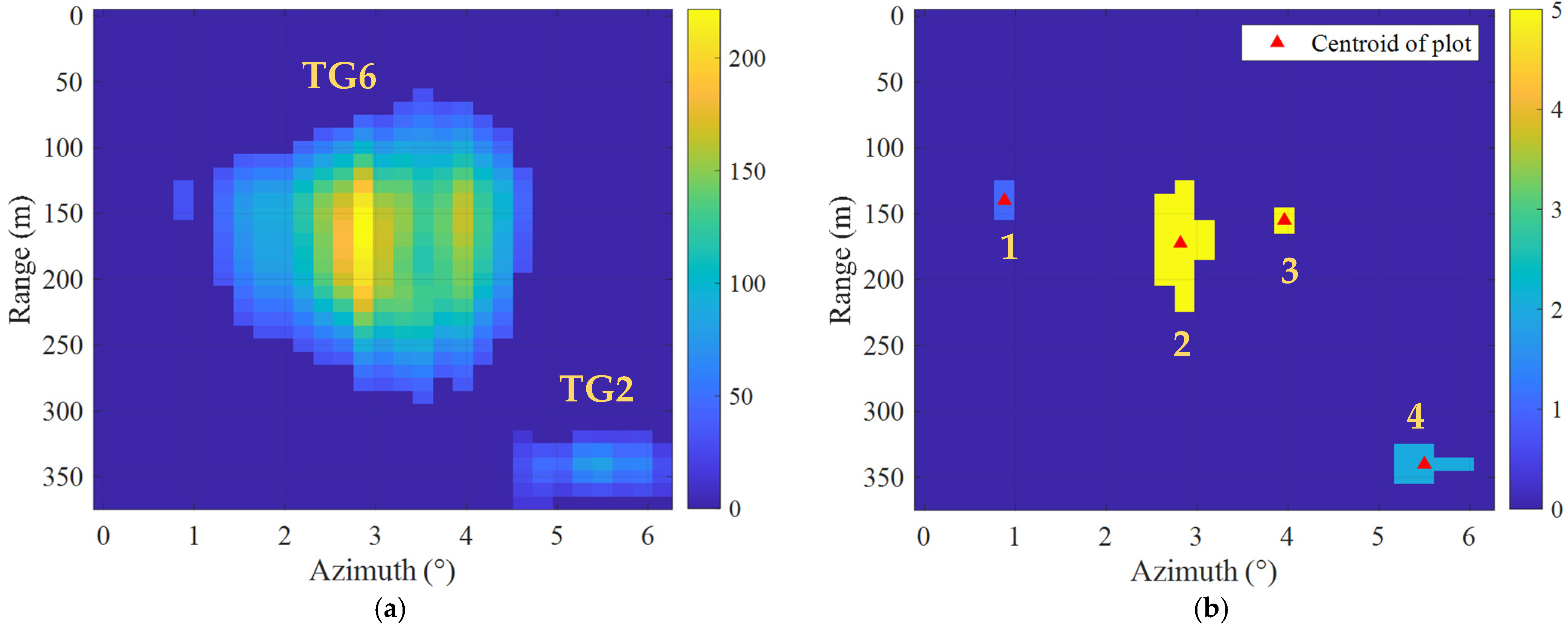
3.1. Estimating Basic Parameters of Targets

The main aim of this module is to estimate the basic parameters of the target, such as the centroid, the reflected energy, and the area of each plot. A block diagram of this module is shown in Figure 5 The detailed steps are written in Algorithm 1. The problem of finding the number of layers L was solved in [17]. The determined parameters are thus as follows: ${\mathsf{\rho }}_{\mathrm{m}\mathrm{a}\mathrm{x}}=200,{\mathsf{\rho }}_{\mathrm{m}\mathrm{i}\mathrm{n}}=20$ and $\mathrm{L}=6$. The functionality of this module was verified with a real single target in [18]. The results of the simulation example (Figure 3a) are shown in Figure 6. The details of the parameters for each plot are listed in

Table 2. Detailed estimated parameters of targets using the proposed and binary methods.

Target	Plot	Proposed Method				Binary Method
		Range r (km)	$\mathbf{Azimuth} \mathit{\alpha }$(°)	Area A (Cell)	Energy E (Layer)	Range r (km)	$\mathbf{Azimuth} \mathit{\alpha }$ (°)
TG1	1	45.14	83.66	4	3	45.136	83.73
TG2	1	44.77	89.98	8	2	44.77	90.10
TG3	1	44.41	75.24	2	3	44.40	76.55
	2	44.41	76.34	1	3
	3	44.41	77.00	1	3
	4	44.41	77.44	2	3
TG4	1	44.22	84.32	4	3	44.21	84.39
TG5	1	43.68	72.63	48	1	44.65	86.46
	2	43.71	75.60	16	5
	3	43.63	75.68	2	5
	4	43.71	76.78	2	3
	5	43.62	77.95	30	1
	6	43.70	78.47	9	1
TG6	1	44.62	84.26	3	1	43.68	75.48
	2	44.65	86.20	20	5
	3	44.64	87.34	2	5
Time (s)	0.21					0.17

. Table 2 shows that the proposed method can estimate each plot’s parameters, such as their positions, area, and energy, while the binary method only provides the target’s position. In addition, the proposed method can solve the binary method’s problem of missing a target (fishing ship). In the next step of the proposed method, a fuzzy logic system was designed to cluster plots based on their parameters. Additionally, the target center coordinates are recalculated.

Algorithm 1 Basic parameter estimation.
Input data: Dataset ${\mathrm{A}}_{\mathrm{n}\mathrm{m}}\left(\mathrm{n},\mathrm{m},{\mathsf{\rho }}_{\mathrm{n}\mathrm{m}}\right)$ Output data: Centroids ${\mathrm{C}}_{\mathrm{i}}\left({\mathrm{r}}_{\mathrm{i}},{\mathsf{\alpha }}_{\mathrm{i}}\right)$, reflected energies ${\mathrm{E}}_{\mathrm{i}}$, and areas ${\mathrm{A}}_{\mathrm{i}}$,
Step 1: Determine the number of layers L based on an image histogram [17]; Step 2: Set upper and lower limits ${\mathsf{\rho }}_{\mathrm{m}\mathrm{a}\mathrm{x}};{\mathsf{\rho }}_{\mathrm{m}\mathrm{i}\mathrm{n}}$ Step 3: Calculate intensity step $∆\mathsf{\rho }$ and intensity value ${\mathsf{\rho }}_{\mathrm{k}}$ of the kth layer using (1) [18].
$\left\{\begin{array}{c}∆\mathsf{\rho }=\frac{{\mathsf{\rho }}_{\mathrm{m}\mathrm{a}\mathrm{x}}-{\mathsf{\rho }}_{\mathrm{m}\mathrm{i}\mathrm{n}}}{\mathrm{L}}\\ {\mathsf{\rho }}_{\mathrm{k}}={\mathsf{\rho }}_{\mathrm{m}\mathrm{i}\mathrm{n}}+k\times ∆\mathsf{\rho }\end{array}\right.$	(1)
Step 4: Encode dataset ${\mathrm{A}\mathrm{T}}_{\mathrm{n}\mathrm{m}}\left(\mathrm{n},\mathrm{m},\mathrm{k}\right)$ using (2).
$\left\{\begin{array}{c} \mathrm{if} {\mathsf{\rho }}_{\mathrm{k}-1}\le {\mathsf{\rho }}_{\mathrm{n}\mathrm{m}}\le {\mathsf{\rho }}_{\mathrm{k}} \mathrm{then} {\mathsf{\rho }}_{\mathrm{k}}\leftarrow {\mathsf{\rho }}_{\mathrm{n}\mathrm{m}}\\ {\mathrm{A}\mathrm{T}}_{\mathrm{n}\mathrm{m}}\left(\mathrm{n},\mathrm{m},\mathrm{k}\right)\leftarrow {\mathrm{A}}_{\mathrm{n}\mathrm{m}}\left(\mathrm{n},\mathrm{m},{\mathsf{\rho }}_{\mathrm{n}\mathrm{m}}\right)\end{array}\right.$	(2)
Step 5: Determine local maximum region ${\mathrm{D}}_{\mathrm{i}}$, for i = 1,.., N, with N as the total local maximum regions [17]. Step 6: Determine centroid ${\mathrm{C}}_{\mathrm{i}}\left({\mathrm{r}}_{\mathrm{i}},{\mathsf{\alpha }}_{\mathrm{i}}\right)$ of ${\mathrm{D}}_{\mathrm{i}}$ using (3), energies ${\mathrm{E}}_{\mathrm{i}}$, and areas ${\mathrm{A}}_{\mathrm{i}}$ of the plots [18].
$\left\{\begin{array}{c}\mathsf{\alpha }=\frac{\sum \left(\mathrm{i}\times \sum {\mathrm{A}}_{\mathrm{i}}\right)}{\sum {\mathrm{A}}_{\mathrm{i}\mathrm{j}}}\\ \mathrm{r}=\frac{\sum \left(\mathrm{j}\times \sum {\mathrm{A}}_{\mathrm{j}}\right)}{\sum {\mathrm{A}}_{\mathrm{i}\mathrm{j}}}\end{array}\right.$	(3)
Where $\sum {\mathrm{A}}_{\mathrm{i}\mathrm{j}}$ is the total number of cells i region D, $\sum {\mathrm{A}}_{\mathrm{i}}$ is the total number of cells in the ith column, and $\sum {\mathrm{A}}_{\mathrm{j}}$ is the total number in the jth row [18].

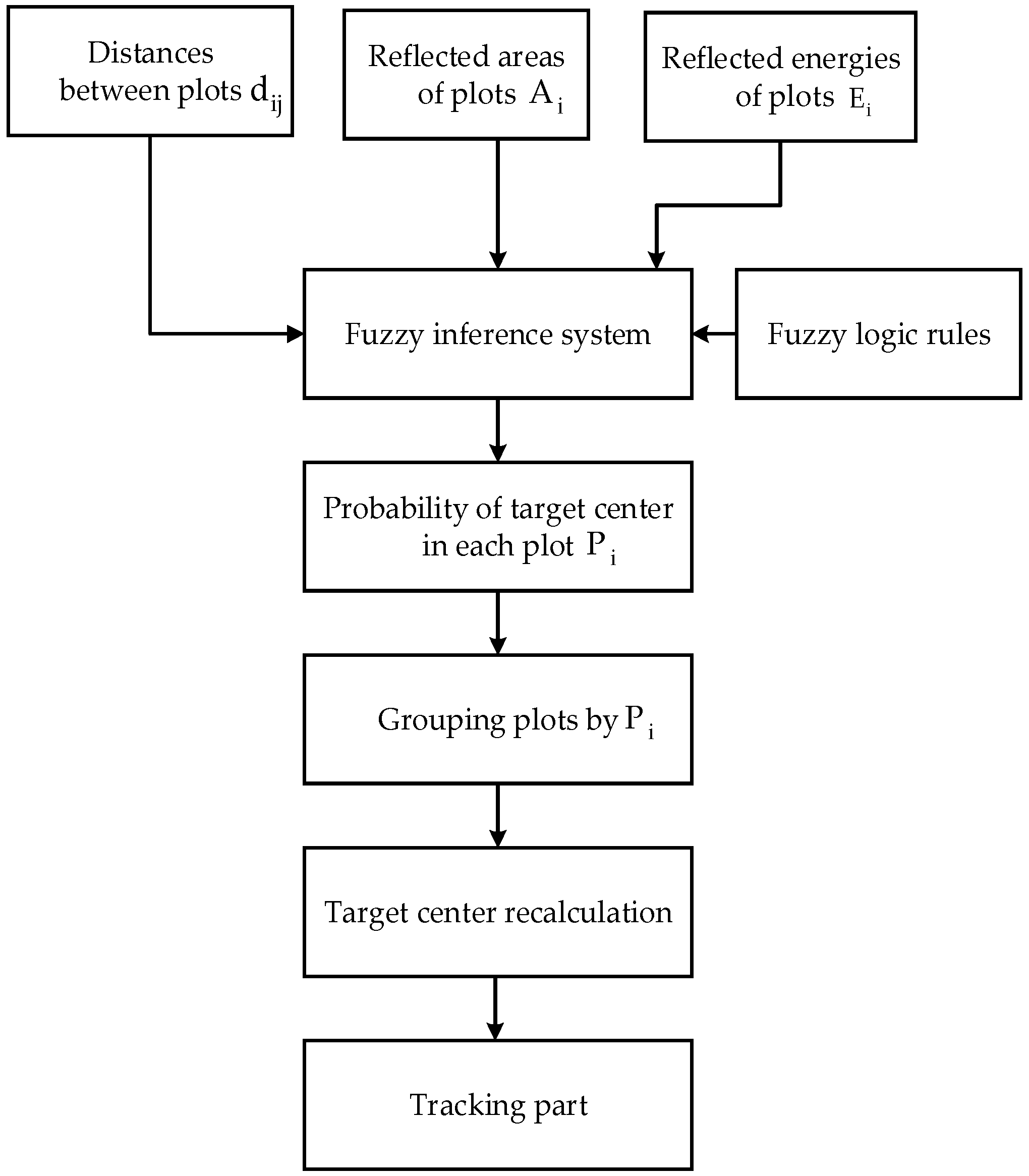
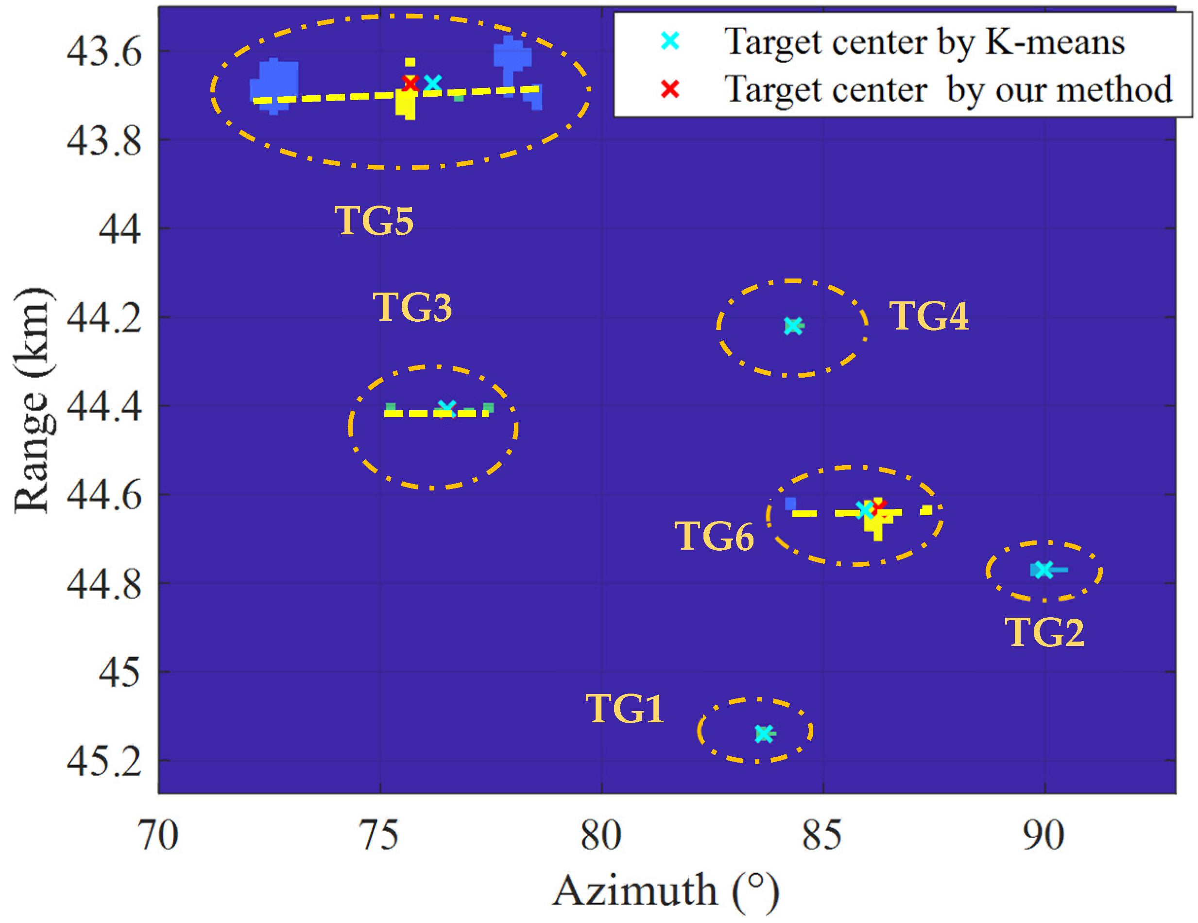
3.2. Clustering Plots and Direction Estimation

A common technique used for clustering plots is the K-means algorithm [19], which requires knowledge of cluster numbers with respect to the number of targets and the use of distances between plots to cluster them in advance. An example of using K-means for clustering plots is shown in Figure 7. Figure 7a shows that the K-means algorithm is effective for clustering plots when the number of clusters is known; the only disadvantage is that the target center coordinates are outside of the area of interest (for high reflected energies, TG5 and TG6). Figure 7b shows that when the number of clusters is unknown, the K-means algorithm does not guarantee accuracy and may not find the correct number of targets (TG2 is grouped into TG6; see Figure 7b). To solve this problem, in this paper, a new method is proposed for clustering plots based on a fuzzy logic system [20] and estimating the characteristics of the plots (FCM-M), presented in Section 3.1. A block diagram of the proposed method is shown in Figure 8, and its steps are noted in Algorithm 2. The inputs of FCM-M are the distance ${\mathrm{d}}_{\mathrm{i}\mathrm{j}}$ between plots, reflected area ${\mathrm{A}}_{\mathrm{i}}$, and energy ${\mathrm{E}}_{\mathrm{i}}$ of the plots. The system’s output is the probability ${\mathrm{P}}_{\mathrm{i}\mathrm{j}}$ that the target’s center of gravity has coordinates in the center of the plot. Each plot uses a fuzzy interface system (FIS) to find this probability.

Algorithm 2 FCM-M for clustering plots.
Input data: Centroids ${\mathrm{C}}_{\mathrm{i}}\left({\mathrm{r}}_{\mathrm{i}},{\mathsf{\alpha }}_{\mathrm{i}}\right)$, reflected energy ${\mathrm{E}}_{\mathrm{i}}$, and area ${\mathrm{A}}_{\mathrm{i}}$, of the plot and threshold value ${\mathrm{P}}_{\mathrm{t}\mathrm{h}}$. Output data: Target center coordinates ${\mathrm{C}}_{\mathrm{c}}\left({\mathrm{r}}_{\mathrm{c}},{\mathsf{\alpha }}_{\mathrm{c}}\right)$ and number of targets N.
Step 1: Design fuzzy logic rules. Step 2: Find the appropriate membership function $\mu \left(x\right)$ for the input data. Step 3: Select a plot ${\mathrm{C}}_{\mathrm{i}}\left({\mathrm{r}}_{\mathrm{i}},{\mathsf{\alpha }}_{\mathrm{i}}\right)$ with the highest reflected energy as the cluster header. Step 4: Calculate distance ${\mathrm{d}}_{\mathrm{i}\mathrm{j}}$ between plots ${\mathrm{C}}_{\mathrm{i}}\left({\mathrm{r}}_{\mathrm{i}},{\mathsf{\alpha }}_{\mathrm{i}}\right)$ and ${\mathrm{C}}_{\mathrm{j}}\left({\mathrm{r}}_{\mathrm{j}},{\mathsf{\alpha }}_{\mathrm{j}}\right)$ using (4)
${\mathrm{d}}_{\mathrm{i}\mathrm{j}}=\sqrt{{\left({\mathrm{r}}_{\mathrm{i}}\cos {\mathsf{\alpha }}_{\mathrm{i}}-{\mathrm{r}}_{\mathrm{j}}\cos {\mathsf{\alpha }}_{\mathrm{j}}\right)}^2+{\left({\mathrm{r}}_{\mathrm{i}}\sin {\mathsf{\alpha }}_{\mathrm{i}}-{\mathrm{r}}_{\mathrm{j}}\sin {\mathsf{\alpha }}_{\mathrm{j}}\right)}^2}$	(4)
Step 5: Calculate the probability of a target center in each plot ${\mathrm{P}}_{\mathrm{i}}$ using (5):
${\mathrm{P}}_{\mathrm{i}}=\frac{\int {\mathsf{\mu }}_{\mathrm{c}}\left(\mathrm{x}\right)\mathrm{x}\mathrm{d}\mathrm{x}}{\int {\mathsf{\mu }}_{\mathrm{c}}\left(\mathrm{x}\right)\mathrm{d}\mathrm{x}}$	(5)
Step 6: Group plots into clusters, CL, using (6).
$\left\{\begin{array}{c}\mathrm{if} \left|{\mathrm{P}}_{\mathrm{i}}-{\mathrm{P}}_{\mathrm{j}}\right|\le {\mathrm{P}}_{\mathrm{t}\mathrm{h}}\\ {\mathrm{C}\mathrm{L}}_{\mathrm{i}}\leftarrow \left({\mathrm{C}}_{\mathrm{i}},{\mathrm{C}}_{\mathrm{j}}\right)\end{array}\right.$	(6)
Step 7: Recalculate the target center coordinates ${\mathrm{C}}_{\mathrm{c}}\left({\mathrm{r}}_{\mathrm{c}},{\mathsf{\alpha }}_{\mathrm{c}}\right)$ using (7):
$\left\{\begin{array}{c}{\mathsf{\alpha }}_{\mathrm{c}}=\frac{\sum _{\mathrm{l}=1}^{\mathrm{K}}{\mathsf{\alpha }}_{\mathrm{l}}{\mathrm{E}}_{\mathrm{l}}}{\sum _{\mathrm{l}=1}^{\mathrm{K}}{\mathrm{E}}_{\mathrm{l}}}\\ {\mathrm{r}}_{\mathrm{c}}=\frac{\sum _{\mathrm{l}=1}^{\mathrm{K}}{\mathrm{r}}_{\mathrm{l}}{\mathrm{E}}_{\mathrm{l}}}{\sum _{\mathrm{l}=1}^{\mathrm{K}}{\mathrm{E}}_{\mathrm{l}}}\end{array}\right.$	(7)
where K is the total number of plots in cluster CL, and the total number of clusters N is known for several detected targets.

Fuzzy Logic Rules

Particularly with a low reflected energy, a small area, and a distance that is very far from the center, the probability of a target center being present in a specific plot is very, very low. To determine such a probability, the basic rules of the fuzzy logic algorithm can be built based on the characteristics of the target as follows:

-

If a plot has a higher reflected energy E and a larger reflected area A, the center of gravity is inside the region of interest. Then, the plot and any close targets can be clustered into one group.

-

If a plot has a lower reflected energy E and a smaller reflected area A, the probability of the target center of gravity being present in the region of interest is low. Thus, the controller can ignore such plots.

-

When two plots have higher reflected energy E and larger reflected area S, a controller can use the probability that a target center is present to decide which plots to track.

Since we have three inputs divided into three levels, an example of 27 fuzzy if–then rules are given in

Table 3. Fuzzy logic rules.

No.	Energy E	Distance D	Area A	Probability P
1	High	Close	Big	Very High
2	High	Close	Medium	Very High
3	High	Close	Small	High
4	High	Medium	Big	High
5	High	Medium	Medium	Medium
6	High	Medium	Small	Medium
7	High	Far	Big	Medium
8	High	Far	Medium	Medium
9	High	Far	Small	Medium
10	Medium	Close	Big	Low
11	Medium	Close	Medium	Very Low
12	Medium	Close	Small	Low
13	Medium	Medium	Big	Medium
14	Medium	Medium	Medium	Medium
15	Medium	Medium	Small	Medium
16	Medium	Far	Big	Medium
17	Medium	Far	Medium	Medium
18	Medium	Far	Small	Medium
19	Low	Close	Big	Medium
20	Low	Close	Medium	Medium
21	Low	Close	Small	Low
22	Low	Medium	Big	Low
23	Low	Medium	Medium	Very Low
24	Low	Medium	Small	Very Low
25	Low	Far	Big	Low
26	Low	Far	Medium	Very Low
27	Low	Far	Small	Very Low

.

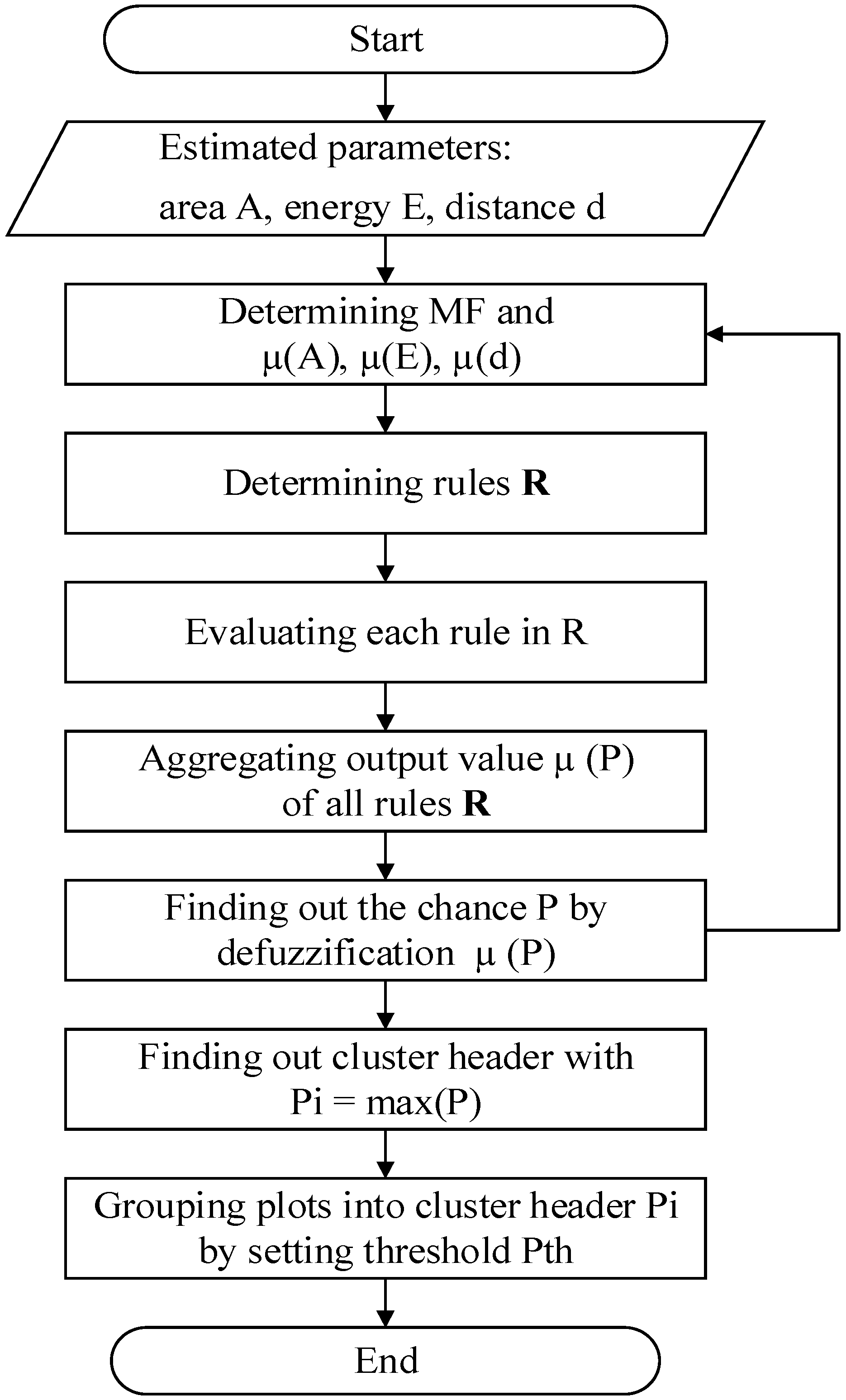
3.3. Fuzzy Logic Membership Functions

The membership functions of FCM-M are trapezoidal, Gaussian, triangular, etc. First, the appropriate membership functions must be chosen. To solve this problem, a scenario is created in Figure 9. In this scenario, the fishing ship (TG2) is next to the container ship (TG6). This problem is not solved with K-means (see Figure 7b). Additionally, the membership functions for the input and output data are shown in Figure 10.

The optimized layer in [17] was 6, so the reflected energy here varied between 1 and 6. The simulation targets were then placed in a 400 m × 6° area. The maximum distance from a plot to the cluster (center) was 400 m. Additionally, the maximum area of the node was in the range of 1 to 20. Details of the parameters of the plots are given in

Table 4. Characteristics of the plots.

Plot ID	Range r (m)	Azimuth α (°)	Area A (cell)	Energy E (layer)
1	150.0	0.88	3	1
2	195.5	2.82	20	5
3	165.0	3.96	2	5
4	345.0	5.55	8	2

. A flowchart of the FCM-M for clustering plots is shown in Figure 11, and the detailed steps are written in Algorithm 3. The chances of an association between plots are listed in

Table 5. Chances of an association between plots.

Plot ID	1st Plot	2nd Plot	3rd Plot	4th Plot
1st Plot		77.34	50	20.80
2nd Plot	77.34		77.74	41.59
3rd Plot	50	77.74		50
4th Plot	20.80	41.59	50

.

Algorithm 3 Detailed steps for clustering plots.

Input data: Estimated area A, energy E of the plots, and distance d between plots. Output data: Chance of each plot being in the region of interest P.

Step 1: Determine the membership function and the probability of each input value $\mathsf{\mu }\left(\mathrm{A}\right)$ $\mathsf{\mu }\left(\mathrm{E}\right)$, $\mathsf{\mu }\left(\mathrm{d}\right)$. Step 2: Determine the fuzzy logic rules R corresponding to each input and output parameter. Step 3: Evaluate every rule in R using the fuzzy definition of AND.

$\mathsf{\mu }\left(\mathrm{A}\right)\mathrm{A}\mathrm{N}\mathrm{D}\mathsf{\mu }\left(\mathrm{E}\right)\mathrm{A}\mathrm{N}\mathrm{D}\mathsf{\mu }\left(\mathrm{d}\right)=\min \left(\mathsf{\mu }\left(\mathrm{A}\right),\mathsf{\mu }\left(\mathrm{E}\right),\mathsf{\mu }\left(\mathrm{d}\right)\right)$

Step 4: Aggregate the output value. Step 5: Find the chance of a plot being in the region of interest using defuzzification (5).

${\mathrm{P}}_{\mathrm{i}}=\frac{\int {\mathsf{\mu }}_{\mathrm{c}}\left(\mathrm{x}\right)\mathrm{x}\mathrm{d}\mathrm{x}}{\int {\mathsf{\mu }}_{\mathrm{c}}\left(\mathrm{x}\right)\mathrm{d}\mathrm{x}}$

Step 6: Select plots with the highest chance ${\mathrm{P}}_{\mathrm{i}}$ of becoming the cluster header and group plots ${\mathrm{P}}_{\mathrm{j}}$ into a cluster header ${\mathrm{P}}_{\mathrm{i}}$ using Pth threshold value.

$\left\{\begin{array}{c}\mathrm{if} \left|{\mathrm{P}}_{\mathrm{i}}-{\mathrm{P}}_{\mathrm{j}}\right|\le {\mathrm{P}}_{\mathrm{t}\mathrm{h}}\\ {\mathrm{C}\mathrm{L}}_{\mathrm{i}}\leftarrow \left({\mathrm{C}}_{\mathrm{i}},{\mathrm{C}}_{\mathrm{j}}\right)\end{array}\right.$

Table 4 shows that the second plot has the highest association chances P = 77.74% with the third plot and P = 77.34% with the first plot, and the lowest chance P = 41.59% for the fourth plot. This means that the first, second, and third plots belong to one target (TG6), and the fourth plot is another target (TG2). The target center coordinates of TG6 are calculated using (8).

$$\left\{\begin{array}{c}{\mathsf{\alpha }}_{\mathrm{c}}=\frac{\sum _{\mathrm{l}=1}^{\mathrm{K}}{\mathsf{\alpha }}_{\mathrm{l}}{\mathrm{E}}_{\mathrm{l}}}{\sum _{\mathrm{l}=1}^{\mathrm{K}}{\mathrm{E}}_{\mathrm{l}}}=\frac{0.88+5\times 2.82+5\times 3.96}{11}=3.16 \left(°\right)\\ {\mathrm{r}}_{\mathrm{c}}=\frac{\sum _{\mathrm{l}=1}^{\mathrm{K}}{\mathrm{r}}_{\mathrm{l}}{\mathrm{E}}_{\mathrm{l}}}{\sum _{\mathrm{l}=1}^{\mathrm{K}}{\mathrm{E}}_{\mathrm{l}}}=\frac{150+182.5\times 5+165\times 5}{11}=171.59 (m)\end{array}\right.$$

(8)

$$\left\{\begin{array}{c}{\mathsf{\alpha }}_{\mathrm{c}}=\frac{\sum _{\mathrm{l}=1}^{\mathrm{K}}{\mathsf{\alpha }}_{\mathrm{l}}{\mathrm{E}}_{\mathrm{l}}}{\sum _{\mathrm{l}=1}^{\mathrm{K}}{\mathrm{E}}_{\mathrm{l}}}=\frac{5.55\times 2}{2}=5.55 \left(°\right)\\ {\mathrm{r}}_{\mathrm{c}}=\frac{\sum _{\mathrm{l}=1}^{\mathrm{K}}{\mathrm{r}}_{\mathrm{l}}{\mathrm{E}}_{\mathrm{l}}}{\sum _{\mathrm{l}=1}^{\mathrm{K}}{\mathrm{E}}_{\mathrm{l}}}=\frac{350\times 2}{2}=350 (m)\end{array}\right.$$

(9)

The target center coordinates of TG2 were recalculated using (9), and the simulation result is shown in Figure 12. Figure 12 shows that FCM-M can solve all of the problems of the K-means algorithm. First, FCM-M can separate two closely spaced targets. In addition, the target center of the coordinate is inside the area with the highest reflected energy (cyan cross line). Moreover, the target has multiple plots (the number of plots is greater than two), and the ship’s longitudinal axis (red line) can be estimated as a line through the target center that connects the two furthest plots.

Similarly, this FCM-M was applied to solve the clustering problem of the scenario in Figure 2b. The estimated parameters of the targets (a ship’s longitudinal axis and center coordinates) are shown in Figure 13 and

Table 6. Target centers estimated with different methods.

	Barycentric Method (Radar)		Binary Method		Proposed Method
	Range r (km)	Azimuth α (°)	Range r (km)	Azimuth α (°)	Range r (km)	Azimuth α (°)
TG1	45.14	83.66	45.136	83.73	45.14	83.66
TG2	44.77	89.98	44.77	90.10	44.77	89.98
TG3	44.41	76.51	44.40	76.55	44.41	76.51
TG4	44.22	84.32	44.21	84.39	44.22	84.32
TG5	44.64	85.93	44.65	86.46	44.64	86.54
TG6	43.68	76.18	43.68	75.48	43.68	75.99

. Figure 13 shows that the estimated target centers are located inside the area with the highest reflected energy (TG5 and TG6, red cross line), while those for K-means are not (cyan cross lines). Additionally, our method gives the same results for small targets (TG1–TG4) as for big targets (multi-plots such as TG3, TG5, and TG6), and our method can estimate their longitudinal axis (yellow line). However, to obtain the characteristics of the targets (center coordinates and the target’s longitudinal axis), our method required a processing time of t = 0.47 s, while that with radar required t = 0.35 s, and the binary method required t = 0.26 s. This means that the traditional methods are faster than ours, but their disadvantage is that they cannot give target direction information.

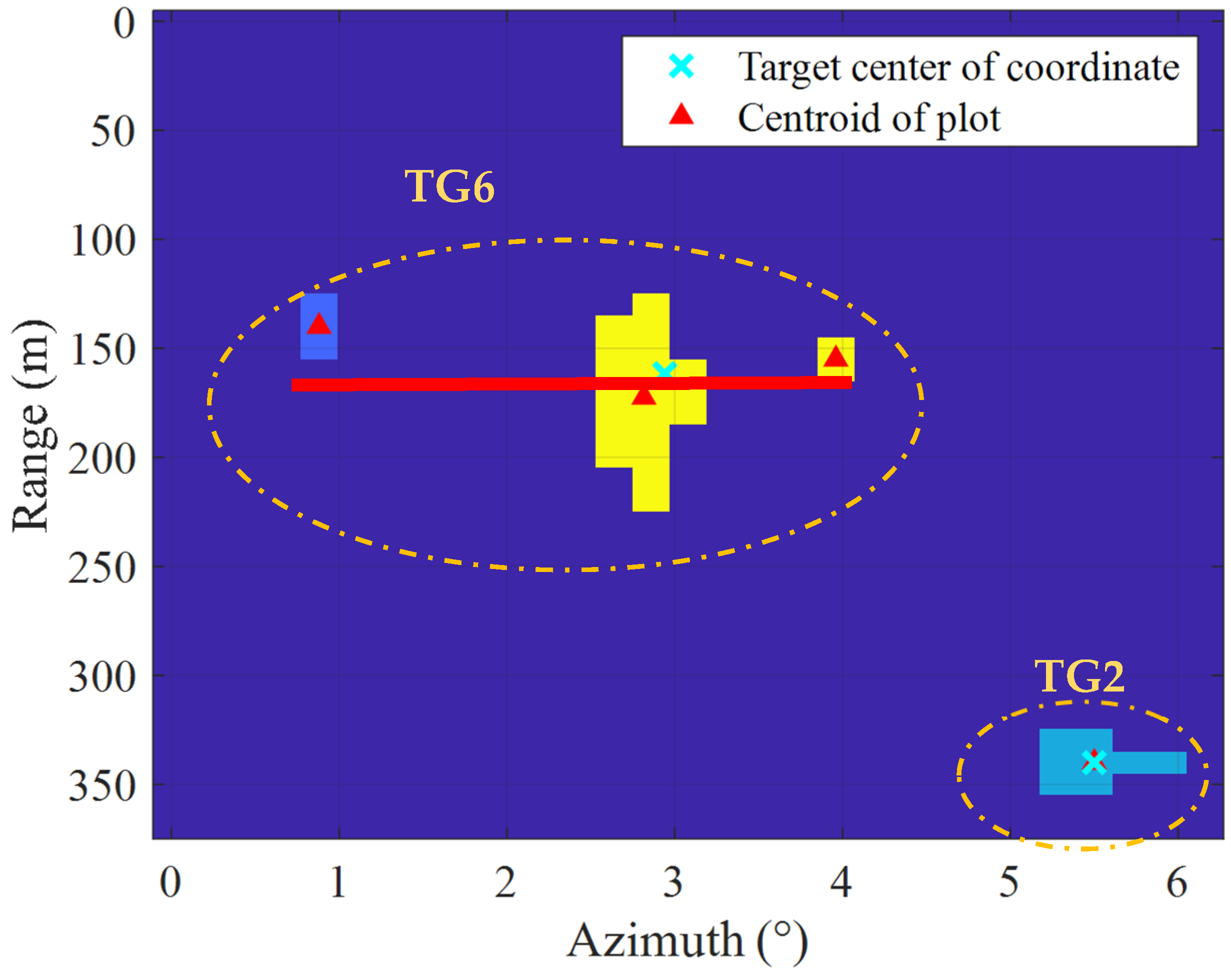
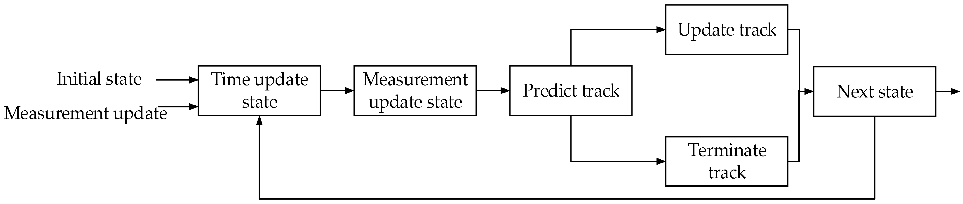
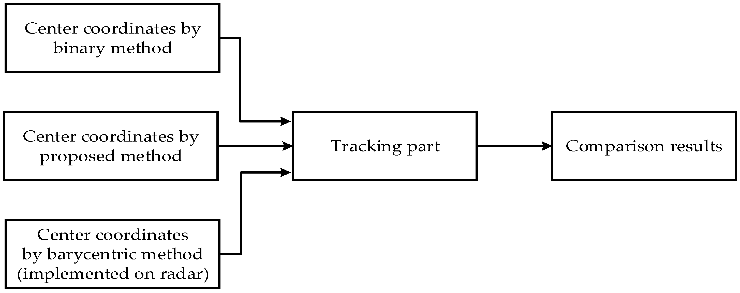
3.4. Target Tracking

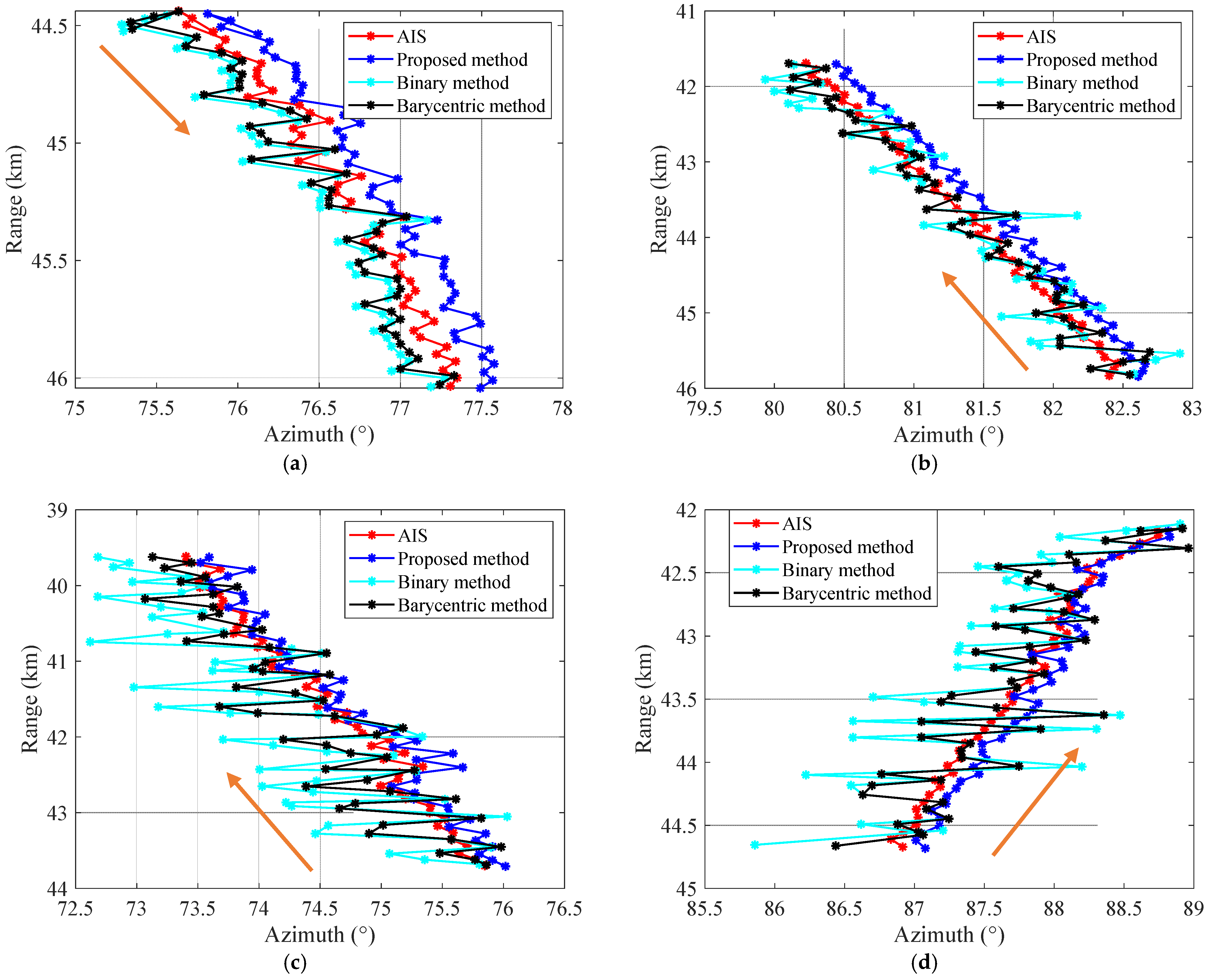
To track selected targets, a Kalman filter is used. A block diagram of the tracking portion is shown in Figure 14. The Kalman filter is written below:

The prediction step is given in (10):

$${\widehat{\mathrm{X}}}_{\mathrm{k}+1/\mathrm{k}}=\mathrm{F}\left(\mathrm{k}\right)\widehat{\mathrm{X}}\left(\mathrm{k}|\mathrm{k}\right)$$

(10)

The predicted error covariance matrix is calculated using (11):

$$\mathrm{P}\left(\mathrm{k}+1|\mathrm{k}\right)=\mathrm{F}\left(\mathrm{k}\right)\mathrm{P}\left(\mathrm{k}|\mathrm{k}\right){\mathrm{F}}^{\mathrm{T}}\left(\mathrm{k}\right)+\mathrm{Q}\left(\mathrm{k}\right)$$

(11)

Using the measured value Z(k+1) at time k + 1, the residual is given in (12):

$$\mathsf{\nu }(\mathrm{k}+1)=\mathrm{Z}\left(\mathrm{k}+1\right)-\mathrm{H}\left(\mathrm{k}+1\right)\widehat{\mathrm{X}}(\mathrm{k}+1|\mathrm{k})$$

(12)

The innovation covariance matrix is given in (13):

$$\mathrm{S}(\mathrm{k}+1)=\mathrm{H}\left(\mathrm{k}\right)\mathrm{P}\left(\mathrm{k}+1\right){\mathrm{H}}^{\mathrm{T}}\left(\mathrm{k}+1\right)+\mathrm{R}(\mathrm{k}+1)$$

(13)

The Kalman gain is calculated using (14):

$$\mathrm{K}(\mathrm{k}+1)=\mathrm{P}\left(\mathrm{k}+1|\mathrm{k}\right){\mathrm{H}}^{\mathrm{T}}\left(\mathrm{k}\right){\mathrm{S}(\mathrm{k}+1)}^{-1}$$

(14)

The updated state vector is calculated using (15):

$$\widehat{\mathrm{X}}\left(\mathrm{k}+1|\mathrm{k}\right)=\widehat{\mathrm{X}}\left(\mathrm{k}+1|\mathrm{k}\right)+\mathrm{K}(\mathrm{k}+1)\mathsf{\upsilon }(\mathrm{k}+1)$$

(15)

The error covariance matrix is updated using (16):

$$\mathrm{P}\left(\mathrm{k}+1|\mathrm{k}+1\right)=\left(\mathrm{I}-\mathrm{K}\left(\mathrm{k}+1\right)\mathrm{H}\left(\mathrm{k}+1\right)\right)\mathrm{P}(\mathrm{k}+1|\mathrm{k})$$

(16)

In this section, the above-mentioned calculated center coordinates of the target ${\mathrm{C}}_{\mathrm{c}}\left({\mathrm{r}}_{\mathrm{c}},{\mathsf{\alpha }}_{\mathrm{c}}\right)$ are used as the input to the tracking portion. The calculated center ${\mathrm{C}}_{\mathrm{c}}\left({\mathrm{r}}_{\mathrm{c}},{\mathsf{\alpha }}_{\mathrm{c}}\right)$ is considered the measured value Z(k+1). To evaluate the proposed method, other methods of calculating target center coordinates were used, such as the binary method with different threshold values and the method implemented on radar (the barycentric method) (see Table 6) fed into the tracking portion (see Figure 15).

To evaluate the proposed method, targets (from TG3 to TG6) were selected for tracking. The AIS trajectories of these targets (50-cycle scans) are shown in Figure 16. The tracked trajectories are shown in Figure 17, and the root mean square errors (RMSEs) of all targets are listed in

Table 7. RMSE errors.

	Proposed Method		Binary Method		Barycentric Method
	Range (m)	Azimuth (°)	Range (m)	Azimuth (°)	Range (m)	Azimuth (°)
TG3	11.05	0.16	38.51	0.20	18.55	0.21
TG4	10.65	0.20	14.46	0.41	13.92	0.32
TG5	7.49	0.12	11.60	0.42	10.39	0.27
TG6	9.89	0.13	21.86	0.58	21.87	0.31
Average	8.59	0.14	21.61	0.41	16.15	0.29

.

Figure 17 and Table 7 show that, in all cases, the best tracked trajectory (close to the original trajectory (red line)) was found using the proposed method (blue line), and the most erroneous result was given by the binary method (cyan line). On the other hand, the results show that the proposed method had higher accuracies for large targets such as targets 4, 6, and 7 (see Figure 17c,d). The proposed method had the lowest average RMSE, ${\mathrm{r}}_{\mathrm{R}\mathrm{M}\mathrm{S}\mathrm{E}}=8.59\left(\mathrm{m}\right)$ in range and ${\mathsf{\alpha }}_{\mathrm{R}\mathrm{M}\mathrm{S}\mathrm{E}}=0.14(°)$ in azimuth, followed by the barycentric method (${\mathrm{r}}_{\mathrm{R}\mathrm{M}\mathrm{S}\mathrm{E}}=16.51\left(\mathrm{m}\right)$ and ${\mathsf{\alpha }}_{\mathrm{R}\mathrm{M}\mathrm{S}\mathrm{E}}=0.29(°)$), and the lowest RMSE was given by the binary method (${\mathrm{r}}_{\mathrm{R}\mathrm{M}\mathrm{S}\mathrm{E}}=21.61\left(\mathrm{m}\right)$ and ${\mathsf{\alpha }}_{\mathrm{R}\mathrm{M}\mathrm{S}\mathrm{E}}=0.41(°)$. They were two times larger than the radar resolution ($\mathsf{\Delta }\mathrm{r}=10\left(\mathrm{m}\right)$ in range and $∆\alpha =0.22(°)$ in azimuth). This confirms that the binary and barycentric methods are ineffective for multi-plot radar images. Overall, all of the methods provided a high level of accuracy for large targets (TG5, TG6).

4. Discussion

In this paper, an algorithm is proposed to estimate the parameters of targets to improve the tracking of their trajectories. The effectiveness of the proposed algorithm was tested with a real-time dataset. The experimental results showed that the proposed method could automatically estimate the target’s parameters, such as the reflected energy and area of each reflected part, and the target’s longitudinal axis. The target’s longitudinal axis is essential for tracking multiple close-space targets.

Firstly, the method determines the local maximum regions of the target radar image using image decomposition. Then, with a fuzzy logic system, the algorithm helps to group plots into each target and to calculate these targets’ center coordinates. The main algorithm is the fuzzy logic system, and target parameters are used to identify two closely spaced targets. Based on these parameters, the target center of the coordinate for the tracking part is calculated.

The proposed method outperformed traditional methods. The average error in the range had an ${\mathrm{r}}_{\mathrm{R}\mathrm{M}\mathrm{S}\mathrm{E}}=8.59\left(\mathrm{m}\right)$ in range and ${\mathsf{\alpha }}_{\mathrm{R}\mathrm{M}\mathrm{S}\mathrm{E}}=0.14(°)$ in azimuth. Additionally, the proposed algorithm was able to overcome the limitations of traditional methods such as having high precision when estimating target centers and providing additional target parameters: reflected area, energy, and especially the target’s longitudinal axis. These parameters, which traditional methods cannot track, play important roles in tracking multiple closely spaced targets. The experimental results also confirmed that the proposed method can be applied to high-resolution radar.

In our subsequent research paper, the movement direction and position of targets will be used to track multiple targets. Additionally, the proposed method will be optimized, especially at the FCM-M stage, to reduce the processing time and to allow the methodology to be gradually implemented in practical applications.

References

1. Liu, C.; Wang, Y. Review of Multi-target Tracking Technology for Marine Radar. J. Radar 2021, 10, 100–115. [Google Scholar] [CrossRef]
2. Beard, M.; Vo, B.T.; Vo, B.N. Bayesian Multi-Target Tracking with Merged Measurement using Labelled Random Finite Sets. IEEE Trans. Signal Process. 2015, 63, 1433–1447. [Google Scholar] [CrossRef]
3. Wang, X.; Gang, L.; You, H. Ship detection in SAR images via local contrast of fisher vector. IEEE Trans. Geosci. Remote Sens. 2020, 58, 6467–6479. [Google Scholar] [CrossRef]
4. Bar-Shalom, Y.; Daum, F.; Huang, J. The probabilistic data association filter. IEEE Control Syst. Mag. 2009, 29, 82–100. [Google Scholar] [CrossRef]
5. Bar-Shalom, Y.; Rong, L.; Kirubarajan, T. Estimation with Applications to Tracking and Navigation: Theory Algorithms and Software; John Wiley & Sons: Hoboken, NJ, USA, 2004; pp. 421–490. ISBN 9780471221272. [Google Scholar] [CrossRef]
6. Mansour, H.; Voicu, G.; Emil, P. The Use of Kalman Filter Techniques for Ship Track Estimation. WSEAS Trans. Syst. 2020, 19, 7–13. [Google Scholar] [CrossRef]
7. Sun, B.; Yan, B.; Jiang, R.; Zhang, J. A progressive update extended Kalman filter for ship tracking with static electric field. J. Natl. Univ. Def. Technol. 2018, 40, 134–140. [Google Scholar] [CrossRef]
8. Wanjin, X.; Liying, L.; Junjie, B.; Yingying, Z. Ship Tracking based on the fusion of Kalman filter and particle filter. In Proceedings of the 2021 the 4th International Conference on Mechatronics and Computer Technology Engineering (MCTE 2021), Xi’an, China, 15–17 October 2021. [Google Scholar] [CrossRef]
9. Zhang, R.; Wang, S.; Lou, Y.; Cheng, L. Integrated Sensing and Communication with Massive MIMO: A Unified Tensor Approach for Channel and Target Parameter Estimation. IEEE Trans. Wirel. Commun. 2024, 99, 1–16. [Google Scholar] [CrossRef]
10. Liu, J.; Wang, Z.; Cheng, D.; Chen, W.; Chen, C. Marine Extended Target Tracking for Scanning Radar Data Using Correlation Filter and Bayes Filter Jointly. Remote Sens. 2022, 14, 5937. [Google Scholar] [CrossRef]
11. Fowdur, J.S.; Baum, M.; Heymann, F. Real-World Marine Radar Datasets for Evaluating Target Tracking Methods. Sensors 2021, 21, 4641. [Google Scholar] [CrossRef] [PubMed]
12. Dang, C.; Li, Z.; Hao, C.; Xiao, Q. Infrared Small Marine Target Detection Based on Spatiotemporal Dynamics Analysis. Remote Sens. 2023, 15, 1258. [Google Scholar] [CrossRef]
13. Fan, E.; Xie, W.; Pei, J.; Hu, K.; Li, X.; Podpečan, V. Improved Joint Probabilistic Data Association (JPDA) Filter Using Motion Feature for Multiple Maneuvering Targets in Uncertain Tracking Situations. Information 2018, 9, 322. [Google Scholar] [CrossRef]
14. Duan, G.; Wang, Y.; Zhang, Y.; Wu, L. A Network Model for Detecting Marine Floating Weak Targets Based on Multimodal Data Fusion of Radar Echoes. Sensors 2022, 22, 9163. [Google Scholar] [CrossRef] [PubMed]
15. Score Coastal Radar. Available online: https://www.radartutorial.eu/19.kartei/07.naval/karte075.en.html (accessed on 1 June 1999).
16. Above Water Warfare. Available online: https://www.thalesgroup.com/en/global/activities/defence/naval-forces/above-water-warfare (accessed on 1 June 1999).
17. Vo, X.H.; Nguyen, T.K.; Nguyen, P.B. Calculating the Optimal Number of Layers for Separating Radar Images of Marine Objects by level. J. Eurasian Union Sci. 2023, 13, 10–20. [Google Scholar] [CrossRef]
18. Vo, X.H.; Nguyen, T.K.; Nguyen, P.B.; Duong, V.M. A Real-time Processing Algorithm for Multi-plot Marine Targets based on Radar Image Decomposition. In Proceedings of the 2023 12th International Conference on Control, Automation and Information Sciences (ICCAIS), Hanoi, Vietnam, 29 November 2023; pp. 781–876. [Google Scholar] [CrossRef]
19. Park, J.; Choi, M. A K-Means Clustering Algorithm to Determine Representative Operational Profiles of a Ship Using AIS Data. J. Mar. Sci. Eng. 2022, 10, 1245. [Google Scholar] [CrossRef]
20. Mendel, J.M. Fuzzy logic systems for engineering: A tutorial. Proc. IEEE 1995, 83, 345–377. [Google Scholar] [CrossRef]
Figure 1. Problems with tracking targets: (a) estimated target center coordinates; (b) problem with multi-target tracking [16].
Electronics 13 02548 g001
Figure 2. Example from the dataset: (a) target TG6; (b) scenario.
Electronics 13 02548 g002
Figure 3. Example of detection results using the binary method: (a) threshold T1; (b) threshold T2.
Electronics 13 02548 g003
Figure 4. A block diagram of the proposed method.
Electronics 13 02548 g004
Figure 5. Block diagram for estimating target parameters.
Electronics 13 02548 g005
Figure 6. Analyzed results of module 1: (a) encoded data; (b) estimated plots.
Electronics 13 02548 g006
Figure 7. Clustered plots based on K-means: (a) six clusters; (b) five clusters.
Electronics 13 02548 g007
Figure 8. FCM-M for clustering plots.
Electronics 13 02548 g008
Figure 9. Scenario for validating membership function: (a) scenario; (b) plots estimated using our method.
Electronics 13 02548 g009
Figure 10. Membership functions of FCM-M: (a) distance d; (b) area A; (c) energy E; (d) chance P.
Electronics 13 02548 g010
Figure 11. A flowchart for clustering plots.
Electronics 13 02548 g011
Figure 12. Results of the first scenario.
Electronics 13 02548 g012
Figure 13. Experimental results of the proposed method.
Electronics 13 02548 g013
Figure 14. A block diagram of the tracking portion.
Electronics 13 02548 g014
Figure 15. Comparison results of all methods.
Electronics 13 02548 g015
Figure 16. Trajectories of all targets (50-cycle scans) obtained with AIS.
Electronics 13 02548 g016
Figure 17. Trajectories tracked using different methods: (a) TG3; (b) TG4; (c) TG5; (d) TG6.
Electronics 13 02548 g017