Abstract
Hyperspectral image classification is widely applied in several fields. Since existing datasets focus on a single scene, current deep learning-based methods typically divide patches randomly on the same image as training and testing samples. This can result in similar spatial distributions of samples, which may incline the network to learn specific spatial distributions in pursuit of falsely high accuracy. In addition, the large variation between single-scene datasets has led to research in cross-scene hyperspectral classification, focusing on domain adaptation and domain generalization while neglecting the exploration of the generalizability of models to specific variables. This paper proposes two approaches to address these issues. The first approach is to train the model on the original image and then test it on the rotated dataset to simulate cross-scene evaluation. The second approach is constructing a new cross-scene dataset for spatial distribution variations, named GF14-C17&C16, to avoid the problems arising from the existing single-scene datasets. The image conditions in this dataset are basically the same, and only the land cover distribution is different. In response to the spatial distribution variations, this paper proposes a constrained spectral attention mechanism and a constrained spatial attention mechanism to limit the fitting of the model to specific feature distributions. Based on these, this paper also constructs a constrained spectral–spatial attention residual network (CSSARN). Extensive experimental results on two public hyperspectral datasets and the GF14-C17&C16 dataset have demonstrated that CSSARN is more effective than other methods in extracting cross-scene spectral and spatial features.
1. Introduction
Hyperspectral images (HSIs) contain hundreds of spectral bands, which allow humans to more accurately identify different materials and objects on the surface [1]. Meanwhile, HSIs have a wide range of applications in many fields, including land-cover classification [2], mineral exploration [3], and environmental monitoring [4]. For instance, HSIs could help distinguish between different types of crops, monitor their health, and identify diseases [5]. In urban planning [6], HSIs are used for the identification and monitoring of buildings and infrastructure.
Deep learning is now widely used in various hyperspectral classification methods. Based on the image features extracted by models, deep learning-based methods can be categorized into spectral feature-based methods, spatial feature-based methods, and spectral–spatial feature-based methods [7]. Spectral feature- and spatial feature-based methods ignore some information, which may delay improving their classification accuracy later. Therefore, the current mainstream method in hyperspectral image classification is the spectral–spatial feature-based deep learning method. This method typically uses an n × n sized patch of the image centered on the pixel to be classified as a sample for the network to extract spatial and spectral features.
Many researchers [8,9,10,11] have utilized spectral–spatial features for hyperspectral image classification. Some researchers [12,13,14] have also found that the current classification accuracies in hyperspectral image classification are overly optimistic, and their generalization ability is poor. The current datasets in the field of hyperspectral image classification are mostly single-scene datasets. Meanwhile, researchers randomly divide training samples and test samples on the same dataset, which leads to the fact that the spatial distribution of land cover in the training samples is similar to that of the test samples. Moreover, this also leads to the fact that the classification accuracy obtained by most of the current algorithms is falsely high at the time of testing. In reality, the spatial distribution of categories in different regions is not the same or similar, and concentrating too much on learning the spatial distribution of land cover in the training samples will lead to network overfitting [15]. Spectral feature-based algorithms do not use spatial information and hence do not have this problem [12]. However, the issue of similar spatial distribution is faced whenever image patches are randomly divided in the same dataset as samples for training and testing.
Figure 1 demonstrates how similar spatial distributions lead to poor generalization. Assuming the size of a hyperspectral image is 7 × 7 × 1, there will be a total of 49 pixels. In Figure 1A, three patches are selected as training samples, and the pixels to be classified in each sample are labeled blue, red, and yellow, respectively. The samples used for training refer to image patches of size 5 × 5 centered on the pixels to be classified, marked by dashed boxes of the same color. It can be seen that the spatial distributions of the three patches are very similar due to overlapping. Secondly, from Figure 1B, it can be seen that when a 3×3 2D convolutional kernel is used in the red patch (as shown in the purple region of the figure), features extracted by the kernel can also be used to discriminate the blue samples due to the shared information source. The presence of overlapping image patches means that they are spatially close enough. According to the first law of geography [16], these samples also make it easier to belong to the same category. As a result, the network may focus too much on learning a specific spatial distribution to achieve an excessively high and false classification accuracy, leading to network overfitting.
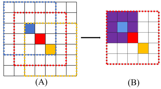
Figure 1.
Diagram of existing problems in hyperspectral image classification. (A) Randomly divided samples lead to similar land-cover distribution. (B) Shared regions produce similar features, which causes the network to tend to learn specific spatial distributions.
To reduce the overfitting problem caused by similar spatial distribution, some researchers have investigated using different sampling strategies [17] to limit the overlap rate between training and testing samples. In addition, reducing the number of training samples [18,19] and decreasing the image patch size [12] can also effectively alleviate this problem. The IEEE Geoscience and Remote Sensing Society (GRSS) also provides the community with the standard train and test split for algorithm evaluation. However, regardless of these methods, the variability of samples selected from the same dataset is limited [20]. Therefore, chosen samples from single-scene datasets cannot wholly avoid spatial distribution similarity, leading to overfitting and poor generalization performance.
Training and testing on single-scene datasets leads to the problem of the similar spatial distribution of samples. Therefore, it is natural to train models with labeled data from one image and test it on the other, which is also closer to real remote sensing applications. This task is called cross-scene hyperspectral classification. The spectrum of the same object may be very different due to many influencing factors in the imaging process [21]. In addition, different datasets are captured in different scenes, which further increases the data distribution differences between images. To deal with the enormous distributional differences, most of the existing research focuses on domain adaptation methods [21,22,23,24] and domain generalization methods [25]. The limitations of single-scene datasets make it challenging for existing studies to assess the generalizability of cross-scene classification concerning individual variables.
The problems in current hyperspectral classification methods and cross-scene hyperspectral classification methods due to the limitations of existing single-scene datasets can be summarized as follows:
- Samples selected from the same image have little spatial variability. As a result, there is an overfitting problem in hyperspectral classification caused by the spatial distribution of training and testing samples being too similar.
- Many cross-scene hyperspectral classification methods focus on domain adaptation and generalization to mitigate the significant data distribution shift between datasets. The lack of univariate cross-scene datasets makes exploring generalization methods for individual variables difficult.
To solve the above issues, this paper proposes two new methods for controlling the variability of the data to the spatial distribution only as shown in Figure 2.
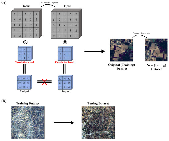
Figure 2.
Schematic of two ideas to mitigate spatial distribution similarity and overfitting. (A) Rotate the image. (B) Cross-scene image dataset.
The first approach is to train the model on the original image and then test it on the rotated dataset to simulate cross-scene evaluation. This is because the output of the same convolutional kernel is not the same when confronted with the same feature at different rotation angles. Previous studies [26] have demonstrated that data augmentation with rotations can only serve to mitigate, rather than address, the sensitivity of the Convolutional Neural Network-based model to spatial rotation. Therefore, even if the training samples are subjected to data augmentation such as rotation, the spatial distribution of the samples before and after rotation remains different for the model. This approach ensures that HSI is free of band number differences, weather differences, and class differences and allows the network to focus only on different features of the spatial distribution of land cover as shown in Figure 2A. It is worth noting that this approach is not a complete substitute for true cross-scene evaluation.
The second method is to construct a univariate cross-scene dataset, which should try to avoid the influence of different numbers of bands, different weather, and different categories on the classification error and focus on the impact of the differences in the spatial distribution of different classes. In this paper, the GF14-C17&C16 dataset was proposed. The images were obtained by the GF-14 satellite from Zhoukou City, Henan Province, China, in April 2022. After atmospheric and radiometric correction, it was manually labeled based on spectral information collected in the field in the city on the day of shooting. The GF14-C17&C16 contains two images, GF14-C17 and GF14-C16, which are different areas of the same city selected from the same satellite image. This ensures consistent image conditions such as acquisition time, atmospheric conditions, and sensor parameters. Further, all labeled feature categories in GF14-C16 are included in GF14-C17, ensuring consistent categories across scene data. Section 4.1 describes more details about this dataset.
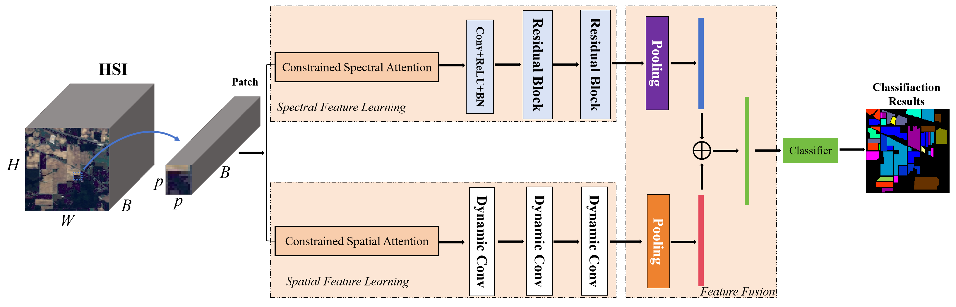
To better deal with spatial variations, this paper proposes a constrained spectral–spatial attention classification residual network (CSSARN) as shown in Figure 3. This network mainly contains a spectral feature learning module, a spatial feature learning module, and a feature fusion module. Since the computation of spectral angles is independent of spatial position, spectral angle mapping is introduced into the spectral attention of the spectral feature learning module. Therefore, this module is robust to spatial rotation, enhancing the generalization of spatial distributions. In the spatial features learning module, a pyramid approach is introduced into the spatial attention to assign higher weights to pixels close to the center pixel. Such an approach weakens the effects caused by spatial variations and thus improves the spatial generalization of the spatial feature learning module.
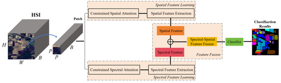
Figure 3.
The structure of the proposed method is named constrained spectral–spatial attention residual network (CSSARN).
This paper has the following contributions.
- 1.
- A novel cross-scene hyperspectral image classification dataset is proposed for the problems of similar spatial distribution of samples caused by using single-scene datasets and the excessive differences between these datasets.
- 2.
- To better deal with spatial variations, we propose a novel attention module consisting of a constrained spectral attention module and a constrained spatial attention module. The former uses spectral angle mapping to constrain the weights of each channel, and the latter uses a pyramidal approach to obtain different spatial weights.
- 3.
- A spectral–spatial attention residual network is constructed based on the above attention module. Single-scene and cross-scene evaluations are performed with public and proposed cross-scene datasets. This network extracts effective spectral–spatial features and has a good generalization of spatial rotations.
The paper is divided into the following sections. Some relevant concepts are briefly described in Section 2. The algorithm is described in detail in Section 3. The experimental results are discussed in Section 4. The proposed cross-scene dataset is also presented in the same section. The discussion and conclusion are drawn in Section 5 and Section 6.
2. Related Works
This section introduces several relevant concepts to explain the proposed CSSARN better.
2.1. Hyperspectral Image Classification
Hyperspectral image classification aims to distinguish the class of each pixel. Early approaches typically used traditional machine learning methods, such as support vector machine (SVM) [27], classification and regression tree (CART) [28], random forest (RF) [29], and extreme learning machine (ELM) [30]. After deep learning was introduced into hyperspectral image classification, it quickly became a mainstream method due to its powerful feature extraction capability [31,32]. Based on the image features extracted by deep learning, they can be categorized into deep learning methods based on spectral features, deep learning methods based on spatial features, and deep learning hyperspectral image classification methods based on spectral–spatial features [7].
Spectral information can help to recognize different feature classes [33,34,35]. It is with this motivation that deep learning methods based on spectral features are proposed. Such methods usually assume that each pixel contains only spectral information about a single object, disregarding spectral mixing, and process each pixel vector in an utterly segregated manner [7,36]. To obtain spectral features, One-Dimensional Convolutional Neural Networks (1D CNNs) [34,37] play an essential role in hyperspectral image classification. This class of methods utilizes 1 × 1 convolutional kernels in Convolutional Neural Networks (CNNs) to extract spectral features and avoid overfitting. Furthermore, some research has employed Recurrent Neural Networks (RNNs) [38] and hybrid convolutional network [39] to extract spectral features.
Methods based on spectral features rely only on spectral information and, therefore, cannot fully utilize the spatial information of the image to describe the distribution of land cover and other information [40]. Due to the limitation of spectral information, another class of methods starts from spatial information to solve the hyperspectral classification problem, called spatial feature-based deep learning methods. Li et al. [41] used principal component analysis (PCA) to extract principal components with spatial information, which were then fed into a CNN for feature learning and classification. Meanwhile, Haut et al. [42] trained a 2D CNN based on spatial features using principal components. Xu et al. [43] proposed a random patches network (RPNet) for hyperspectral image classification. Bera et al. [44] found that although spatial information can improve classification accuracy, it cannot fully identify small objects. Whereas the spectral profiles differ between different objects, the spectral features of even small objects help distinguish their categories.
Although the above algorithms have made significant progress in hyperspectral image classification, both ignore some information, which may result in difficulties in improving their classification accuracy at a later stage. The current mainstream algorithms in this field are based on deep learning methods combining spectral–spatial features. Ghamisi et al. [45] demonstrated that introducing spatial information into the structure of a network based on spectral features helps to improve classification accuracy. Paoletti et al. [32] proposed a novel ResNet based on pyramidal bottleneck residual units, which uses spatial and spectral information for hyperspectral classification. Zheng et al. [26] proposed a central spectral attention mechanism to obtain spectral features, used a spatial similarity approach to obtain spatial features of the image, and finally fused the two features for hyperspectral classification. Liu et al. [46] proposed scaled dot-product central attention for extracting spectral–spatial information.
In addition to the above methods, several studies have used GAN [47], ViT, and other methods. Mei et al. [48] used an unsupervised 3D CNN autoencoder to extract spectral–spatial features. Vision Transformers (ViTs) [49] have shown impressive performance in various tasks in computer vision. Hyperspectral images, with their large number of continuous spectral bands, can be regarded as long-range sequence elements, and ViTs can effectively model long-range interactions and flexibly adjust their receptive fields to cope with interferences in the data, so ViTs have been introduced to the spectral–spatial feature extraction of hyperspectral images by many scholars. He et al. [50] proposed a Transformer-based bi-directional encoder network, which can effectively capture global features. Zhong et al. [51] used a spectral–spatial Transformer network, mainly composed of a spatial attention module and a spectral connection module. Roy et al. [52] proposed a new morphFormer that uses spectral and spatial morphological convolution operations to fuse information from CLS tokens and HSI patch tokens.
2.2. Cross-Scene Hyperspectral Image Classification
In real remote sensing applications, using labeled data from one dataset for training and testing on another is common, and it is called cross-scene hyperspectral image classification. The same object’s spectral distributions may differ due to many influencing factors in the imaging process [21]. In addition, different datasets are captured in different scenes, which further increases the data distribution differences between images.
To deal with the enormous distributional differences, most of the existing research focuses on domain adaptation methods [21,22,23,24] and adaptation generalization [25]. Samat et al. [22] experimentally studied the suitability of geodesic flow Gaussian kernel for unsupervised domain adaptation to deal with the domain shift problem. Shen et al. [23] proposed a new domain adaptation method called hyperspectral feature adaptation and augmentation (HFAA) to solve the dataset shift problem between datasets collected from two different but similar scenes. Zhong et al. [21] proposed a domain adaptation method based on the probability distribution of statistics to reduce the distribution distance between the source image and the target image captured. To deal with the problem that CNN-based methods do not capture nonlocal topological relationships, Zhang et al. [24] developed a Topological structure and Semantic information Transfer network (TSTnet) based on a graph convolution network (GCN). In addition, Zhang et al. [25] also proposed, for the first time, a domain generalization framework for cross-scene HSI classification. It is based on generative adversarial learning, which only needs to use the source domain data to train the model and generalize it to the target domain.
Due to the limitations of single-scene datasets, the problem of data distribution shift is prominent in cross-scene hyperspectral image classification. Therefore, researchers study methods such as domain adaptation and domain generalization to address the significant differences between datasets, neglecting the study of univariate generalizability in cross-scene classification.
3. Proposed Method
In this section, the components of the proposed algorithm are described in detail. Section 3.1 briefly introduces the overall network structure. The spectral feature learning module and spatial feature learning module are reported in Section 3.2 and Section 3.3, respectively. The loss function is explained in Section 3.4.
3.1. Overview
Considering that the HSI is a three-dimensional cube [53], it is assumed that denotes the HSIs, where represents the spatial size of the image. is the number of bands. The is the land-cover classes. represents the number of categories.
As shown in Figure 3, the constrained spectral–spatial attention residual network (CSSARN) mainly consists of a spatial feature learning module, a spectral feature learning module, and a feature fusion module. These modules are described in detail subsequently. Specifically, the spectral feature learning module includes the constrained spectral attention mechanism and the spectral feature extraction module. The constrained spectral attention module uses spectral angle mapping to generate adaptive spectral attention weights, which reduces interference between different categories. Then, the spectral features are extracted by a spectral feature extraction module constructed from residual blocks. At the same time, the spatial feature learning module includes a constrained spatial attention mechanism and a spatial feature extraction module. Constrained spatial attention uses a pyramidal approach to obtain different spatial weights. The spatial features are then extracted by a spatial feature extraction module constructed from the residual block consisting of dynamic convolution. Finally, the spectral and spatial features are fused and fed into the classifier to complete the classification.
3.2. Spectral Feature Learning Module
The spectral feature learning module focuses on spectral information. It mainly includes a constrained spectral attention mechanism and a spectral feature extraction module. Spectral attention mechanisms are widely used in hyperspectral image classification. For instance, Shi et al. [54] utilized the spectral attention mechanism as a band selection module that adaptively selects spectral features important for classification. Zheng et al. [26] proposed a center spectral attention to suppressing redundant channels. The scholars [51,55,56] introduced a novel spectral–spatial attention network to capture pixel correlations. Several works [57,58,59] have also confirmed the effectiveness of the spectral attention mechanism for extracting spectral features.
Nevertheless, as shown in Figure 4A, the common spectral attention mechanisms [46,54,60] use the full spectral information in calculating the spectral band weights. HSIs have a lower spatial resolution compared to RGB images. Therefore, an HSI contains multiple land cover classes with different spectral information. In Figure 4A, the global average pooling operation computes spectral information for all categories on a single image. When calculating the spectral band weights, if all the spectral information is utilized, it may interfere with the recognition of the center pixel.
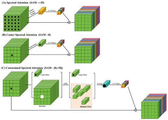
Figure 4.
Structural diagram of several different spectral attention. (A) Spectral attention. (B) Center spectral attention. (C) Constrained spectral attention. The constrained spectral attention is proposed in this paper.
To avoid the interference of spectral information between different categories, Zheng et al. [26] proposed a central spectral attention mechanism as shown in Figure 4B. This method directly uses the center pixel to generate the weight of the spectral attention mechanism. This attention mechanism can prevent information interference between different categories. However, it is common to encounter situations where the same class has different spectra in HSIs. Relying solely on the spectral information of the center pixel may cause the network to overfit the spectral features of the center pixel, leading to poor generalization.
To be able to generate appropriate spectral attention weights, this paper proposes a novel spectral attention mechanism named constrained spectral attention as shown in Figure 4C. The constrained spectral attention utilizes spectral angle mapping (SAM) [61] to measure the similarity of the center pixel to other surrounding pixels. The SAM is calculated as follows:
where denotes the center pixel. The is the other surrounding pixels. The smaller SAM means more similarity between two spectral vectors.
The SAM is utilized to measure the similarity between two spectral features. Consequently, the spectral angles between the surrounding pixels and the center pixel in an image patch can be computed, and a spectral angle threshold can be employed to determine whether the surrounding pixels are similar to the center pixel. Furthermore, the spectral angle of two pixels below the threshold indicates that the angle between the two spectral vectors is sufficiently small to have a high probability of belonging to the same class, thereby allowing them to be judged as similar and vice versa. The center pixel is utilized as the standard, while similar surrounding pixels are retained, and nonsimilar ones are discarded. The similar surrounding pixels are average pooling with the center pixel to derive a weight for the spectral attention mechanism. This weight is multiplied pixel by pixel with the original HSI to obtain the corrected spectral features. It is worth noting that the constrained spectral attention proposed in this paper degrades to the central spectral attention when the threshold of SAM → 0; when the threshold of SAM → , the constrained spectral attention also degrades to the spectral attention.
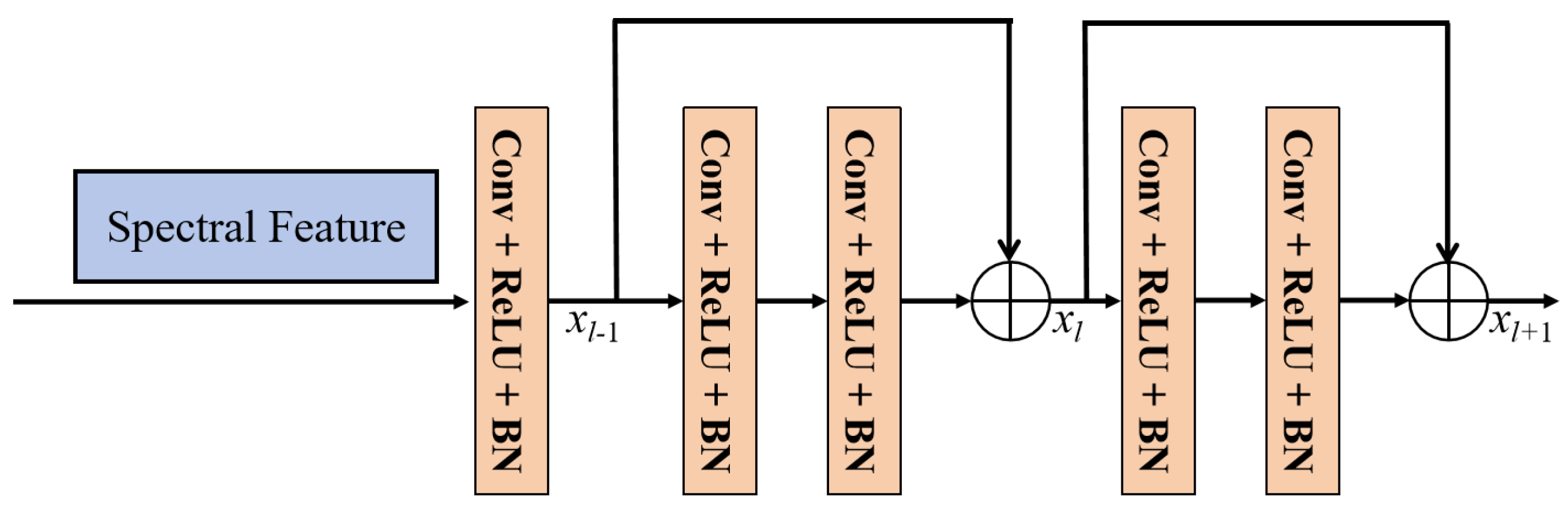
The spectral information undergoes spectral attention to form preliminary spectral features, and the deeper spectral features are learned using a spectral feature extraction network constructed from the residual module. The spatial size of the convolution kernel in the spectral feature learning module is set to 1 × 1 to avoid the interference of spatial information. Figure 5 shows the residual structure of the spectral feature extraction module, which consists of two residual blocks. The use of residual blocks avoids the problem of information loss as the network depth deepens [62,63]. Equations (2) and (3) represent the computation process of the residual module:
where , and represent the output features of layer , layer l and layer , respectively. and correspondingly denote the feature learning modules of layer l and layer , which are used to learn features from the output features of layer and layer l. and are the weight parameters and bias of layer l and layer .
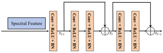
Figure 5.
The structures of the spectral feature extraction module.
The spectral information is passed through the spectral feature learning module, and the output feature is fed into the feature fusion module for spectral–spatial feature fusion.
3.3. Spatial Feature Learning Module
The spatial feature learning module focuses on spatial information. It mainly includes a constrained spatial attention mechanism and a spatial feature extraction module. The commonly used spatial attention is shown in Figure 6A, which uses global average pooling and maximum pooling to obtain the spatial information weights and then extracts the spatial features of HSIs. This spatial attention considers the effect on the center pixel to be the same for all positions in space.
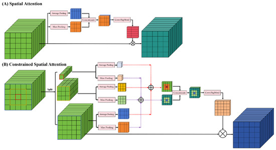
Figure 6.
Structural diagram of different spatial attention. (A) Spatial attention. (B) Constrained spatial attention. The constrained spatial attention is proposed in this paper.
The land cover distribution of HSIs has spatial continuity and smoothness. It means that pixels close to the center location have a high likelihood that their category is the same as the center pixel. The pixels further away from the center position are less likely to have the same category as the center pixel. Therefore, the effect of each location in space on the center pixel is not the same. Hence, as shown in Figure 6B, we propose a new spatial attention named constrained spatial attention in this paper.
The constrained spatial attention divides the HSI into n blocks, where . represents the size of the spatial feature. stands for rounding up. For instance, the size of the spatial feature is . The spatial features are divided into three blocks. The first block is the center pixel. The second block adds a new layer of spatial pixels around the first block. The third block adds a new layer of spatial pixels around the second block. Maximum pooling and global average pooling are performed for each block. Then, the individual pooling features are summed at the corresponding positions in a pyramid–stacked form. Spatial feature learning uses stacked features as weights for spatial attention.
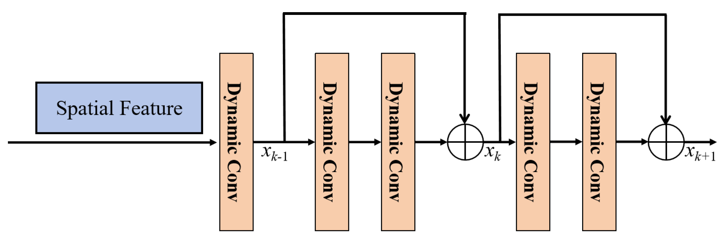
Figure 7 shows that the spatial feature extraction module consists of multiple dynamic convolutional layers [64,65,66]. These dynamic convolutional layers are comprised of two residual blocks. Equations (4) and (5) represent the computation process of the dynamic convolutional residual block:
where , and represent the output features of layer , layer k and layer , respectively. and correspondingly denote the feature learning modules of layer k and layer , which are used to learn features from the output features of layer and layer k. and are the weight parameters and bias of dynamic convolutional layer k and dynamic convolutional layer .
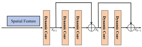
Figure 7.
The structures of the spatial feature extraction module.
The spatial information is passed through the spatial feature learning module, and the output feature is fed into the feature fusion module for spectral–spatial feature fusion.
3.4. Feature Fusion and Loss Function
After obtaining the spatial and spectral features of the HSI, respectively, they are fused by the feature fusion module. The computational process is as follows:
where denotes the spatial features. stands for spectral features. is the fused features. Finally, the fused features are fed into the Softmax classifier to complete the classification:
where are the prediction categories. and denote the ith and jth feature vectors in the fused feature, respectively. That means the category with the largest probability value is the prediction category of the network.
In hyperspectral image classification, the commonly used loss function is cross-entropy loss [15,54,67,68]. Hence, this paper also adopts the cross-entropy loss function to constrain the optimization process. The mth iteration of the training loss calculation process can be expressed as:
where represents the m-th loss. and denote the t-th patch cube and corresponding category label. denotes the softmax layer. T is the number of samples in the training batch. C denotes the number of classes. represents the indicator function. If the condition is satisfied, the indicator function equals one.
The proposed CSSARN consists of the above three modules. It is constrained to train using the cross-entropy loss function. The overall network structure is shown in Figure 8.

Figure 8.
Flowchart of the constrained spectral–spatial attention residual network.
4. Results
In this section, the constrained spectral–spatial attention residual network (CSSARN) proposed in this paper is experimented on the two public datasets, and a novel proposed cross-scene dataset named GF14-C17&C16. In the meantime, the common and the latest methods are selected as comparison algorithms. Specifically, the datasets and evaluation metrics are described in Section 4.1. The experimental setup and compared methods are described in Section 4.2. Then, in Section 4.3, the parameter analysis experiment and ablation experiments are carried out. Finally, the results of the experiments are derived in Section 4.4.
4.1. Data Description and Evaluation Metrics
4.1.1. Data Description
- Indian Pines: The Indian Pines (IP) dataset has a spatial size of 145 × 145 and contains 200 spectral bands that can be used for experiments. The wavelength range of this dataset is 400–2500 nm. A total of 10,249 samples from 16 different classes are included. The number of training and testing samples on the IP dataset is listed in Table 1. Figure 9a,b show the false-color composite image and ground truth of the IP dataset, respectively.
 Table 1. The number of training and testing samples on the Indian Pines (IP) dataset.
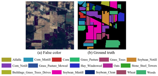 Figure 9. Indian Pines dataset. (a) False-color composite image. (b) Ground truth.
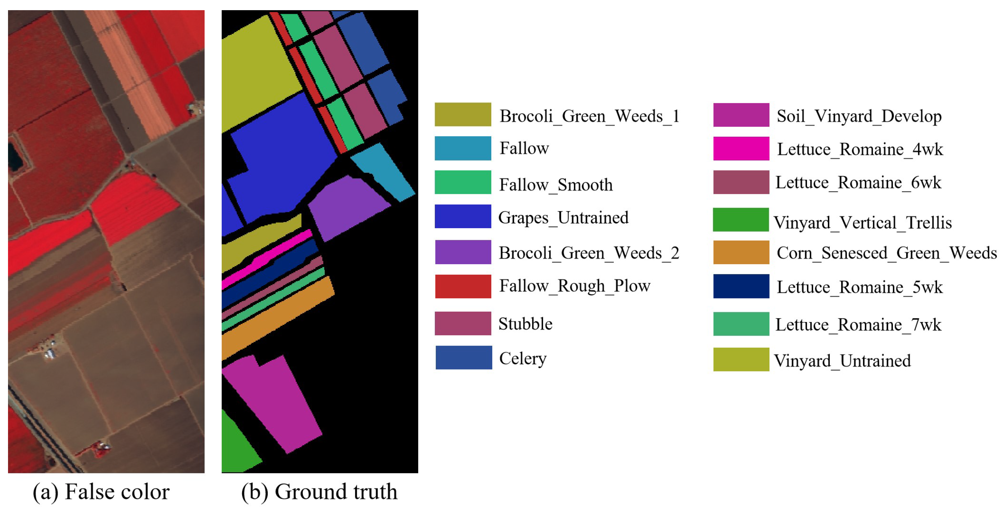
 - Salinas: The Salinas (SA) dataset has a spatial size of 512 × 217 and contains 204 spectral bands that can be used for experiments. The wavelength range of this dataset is 400–2500 nm. A total of 54,129 samples from 16 different classes are included. Table 2 shows the number of training and testing samples on the SA dataset. Figure 10a,b show the false-color composite image and ground truth of the SA dataset, respectively.
Table 2. The number of training and testing samples on the Salinas (SA) dataset.
 Figure 10. Salinas dataset. (a) False-color composite image. (b) Ground truth.
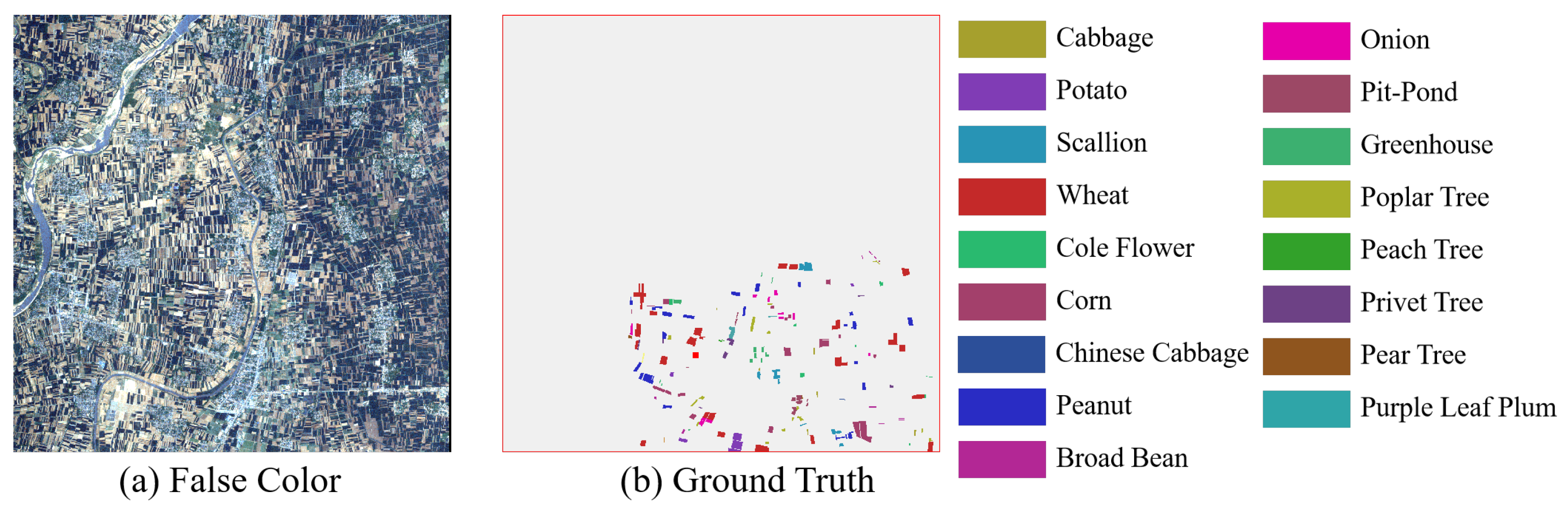
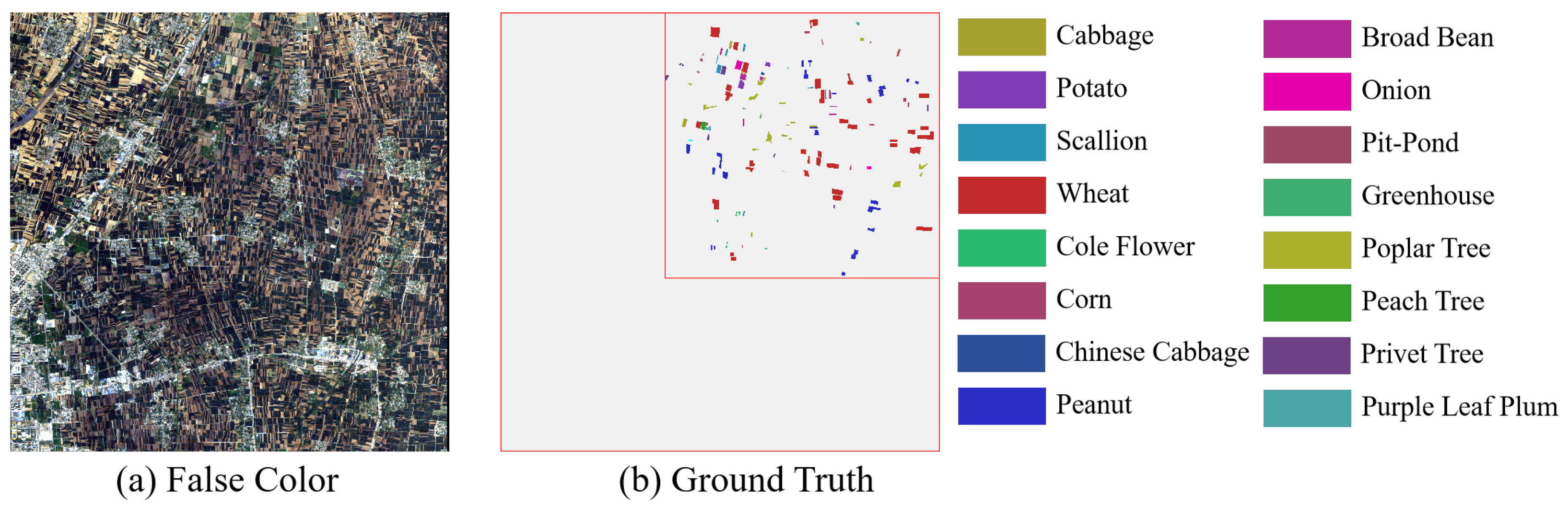
 - GF14-C17&C16: The GF14-C17&C16 dataset was obtained by the GF-14 satellite from Zhoukou City, Henan Province, China, in April 2022. After atmospheric and radiometric correction, it was manually labeled based on spectral information collected in the field in the city on the day of shooting. The GF14-C17&C16 dataset contains 70 spectral channels. The spatial resolution is 5 m per pixel. The spatial size of GF14-C17&C16 is 2048 × 2048. The wavelength range of this dataset is 450–900 nm. There are 80,653 samples in the GF14-C17, which contains 17 categories. A total of 58,550 samples from 16 different classes are included in GF14-C16. Table 3 shows the number of training and testing samples on the GF14-C17&C16 dataset. In this paper, 1606 samples are randomly selected in GF14-C17 as training samples, and the remaining samples of GF14-C17 with all the samples of GF14-C16 are used as test samples. Figure 11a,b show the false-color composite image and ground truth of the GF14-C17 dataset, respectively. The false-color composite image and ground truth of the GF14-C16 dataset are respectively shown in Figure 12a,b.
Table 3. The number of training and testing samples on GF14-C17&C16 dataset.
 Figure 11. GF14-C17 dataset. (a) False-color composite image. (b) Ground truth.
 Figure 12. GF14-C16 dataset. (a) False-color composite image. (b) Ground truth.
4.1.2. Evaluation Metrics
In this paper, three common metrics [54] for classification have been chosen to evaluate each algorithm, mainly including overall accuracy (OA), average accuracy (AA), and Kappa coefficient (). Larger values of these indicate better results.
- Average accuracy (AA):where denotes the confusion matrix. n represents the number of classes.
- Overall accuracy (OA):
- Kappa coefficient ():where represents the i-th row and j-th column of the matrix . The value of denotes the i-th category is classified as the j-th class. ∑ stands for summation.
4.2. Experimental Setup and Compared Methods
4.2.1. Experimental Setup
All methods are experimented on a single NVIDIA GeForce RTX 3090 Graphics Processing Unit (GPU) with 24 GB of memory and a Center Processing Unit (CPU) with 512 GB of memory. The programming language used is Python 3.9.13, and the version of the machine learning library is Pytorch 1.12.1. The number of training sample iterations for all algorithms is 200, and each batch has 64 training samples fed into each network for feature learning. The proposed CSSARN network uses the Adam optimizer with default values. The weight decay factor of the optimizer is 5 × 10⁻⁵, the initial learning rate used is 0.001, and the values of beta1 and beta2 are set to 0.9 and 0.999, respectively. The learning rate is multiplied by a decay factor of 0.6 after every 10 iterations. The loss function used is cross-entropy loss. The optimizer, learning rate, and loss function used in the comparison algorithm are set according to the parameters given in the original literature to ensure the fairness of the experiment.
Let denote the HSI. The and represent the spatial dimensions of height and width. And represents the number of bands. In the data preprocessing stage, all the values are normalized to the [0,1] using Equation (13). After normalization, the required training samples are generated according to the data generation approach utilized by [15]:
where and represent the minimum and maximum value of the HSI.
4.2.2. Compared Methods
The comparison methods can be classified into CNN-based and Transformer-based, depending on the network structure utilized. CNN-based algorithms include 1D CNN [34], 3D CNN [69], DFFN [70], RSSAN [71], Bi-LSTM [60], and RIAN [26]. Transformer-based comparison algorithms include SF [72] and GAHT [68]. The parameter settings for experiments of all comparison methods are set according to the best settings in the original paper.
4.3. Parameter Analysis and Ablation Experiments
4.3.1. Parameter Analysis
This section analyzes how parameters affect the effectiveness of the proposed method. Two hyperparameters, the threshold of SAM and image block size, affect the network classification accuracy. Therefore, this section explores their effects on classification accuracy.
Table 4 shows the effect of SAM on the OAs. It can be seen that different datasets require different SAM values. Because different datasets have different spatial resolutions, each pixel does not contain the same categories. Therefore, the appropriate SAM needs to be determined for each dataset. It is worth noting that when SAM = 0, the constrained spectral attention proposed in this paper becomes the central spectral attention. When SAM = , the proposed constrained spectral attention becomes the spectral attention. Regardless of the dataset, the OA is not the highest when SAM = 0 or SAM = . Based on the results in Table 4, the threshold of SAM is set to 0.6.
Table 4.
The OAs (%) for CSSARN for different SAM on different datasets.
The size of the image block implies the amount of spatial information contained and affects the network training time and inference speed. An image block size that is too large means that the network may require more parameters, take up more computational resources and computation time, and introduce irrelevant sample information, leading to a decrease in OA. An image size that is too small may result in the network being unable to thoroughly learn the required semantic information, leading to low OA.
Table 5 lists the OAs of the CSSARN for different image block sizes. For classification results on the SA dataset, the image block size with the highest OA for CSSARN is 13 × 13. The highest OA for CSSARN on the IP and GF14-C17 is an image block size of 11 × 11. Because of the higher spatial resolution of the SA dataset, it contains more spatial information when the spatial size is larger. While the spatial resolution of IP and GF14-C17 is lower than SA, when the spatial size is too large, it can easily contain more mixed pixels, thus leading to lower OA. Based on the results in Table 5, the patch size is set to 11.
Table 5.
The OAs (%) for CSSARN for different patch sizes on different datasets.
4.3.2. Ablation Experiments
This paper proposes two new attention mechanisms: constrained spectral and spatial attention. Based on this, the constrained spectral–spatial attention residual network is constructed. The corresponding ablation experiments are conducted in this section to verify the effect of the above attention mechanisms. Details of ablation experiments are as follows:
- Base: This network is the CSSARN after removing the constrained spectral attention and the constrained spatial attention.
- Constrained Spatial Attention Network (SpaANet): The constrained spatial attention module is added to the baseline network.
- Constrained Spectral Attention Network (SpecANet): The constrained spectral attention module is added to the baseline network.
- CSSARN: The whole network.
Table 6 shows the results of the ablation experiment. It is easy to see that each attention module improves the overall accuracy of the classification on different datasets. Compared to the base network, the SpaANet increases the OAs by 1.18%, 1.03%, 1.26%, and 2.04%. It shows that using constrained spatial attention facilitates capturing more efficient spatial features to improve the OAs. Also, compared to the base network, the SpecANet increases the OAs by 1.43%, 0.77%, 1.19%, and 2.50%. It demonstrates that the use of constrained spectral attention could increase the weights of important spectral features, which in turn improves the OAs. The CSSARN OAs are 0.72%, 0.06%, 0.26%, 1.89% better than those of the SpaANet, and 0.47%, 0.32%, 0.33%, and 1.43% better than those of the SpecANet, respectively. This indicates that using the two constrained modules together is beneficial in improving the OA of the classification.
Table 6.
The OAs (%) of the network formed by each module on the different datasets.
4.4. Experimental Results
This section shows the OAs, AAs, single-category classification accuracy, and Kappa coefficients of each algorithm on both public and GF14-C17&C16 datasets. In the meantime, the visualization results of each algorithm on each dataset are shown. To achieve a similar effect to cross-scene testing on a single-scene dataset, we train and test the CSSARN on the original image and test again after rotating the original image by 180° for the public dataset. For convenience of presentation, the rotated dataset is referred to as the new dataset in this paper. Meanwhile, comparative experiments about data augmentation are also conducted on IP and SA datasets to determine the efficacy of data augmentation in addressing spatial variations, including rotation. The data augmentation method follows Zheng et al. [26], whereby the samples in the training set are rotated by 0°, 90°, 180°, and 270° to increase the diversity of the training set. Subsequently, the test sample is rotated by 0°, 90°, 180°, and 270°, respectively, to evaluate the performance of the comparison methods. For the GF14-C17&C16, the CSSARN is first trained on GF14-C17 and then tested on GF14-C17 and GF14-C16 separately.
- 1.
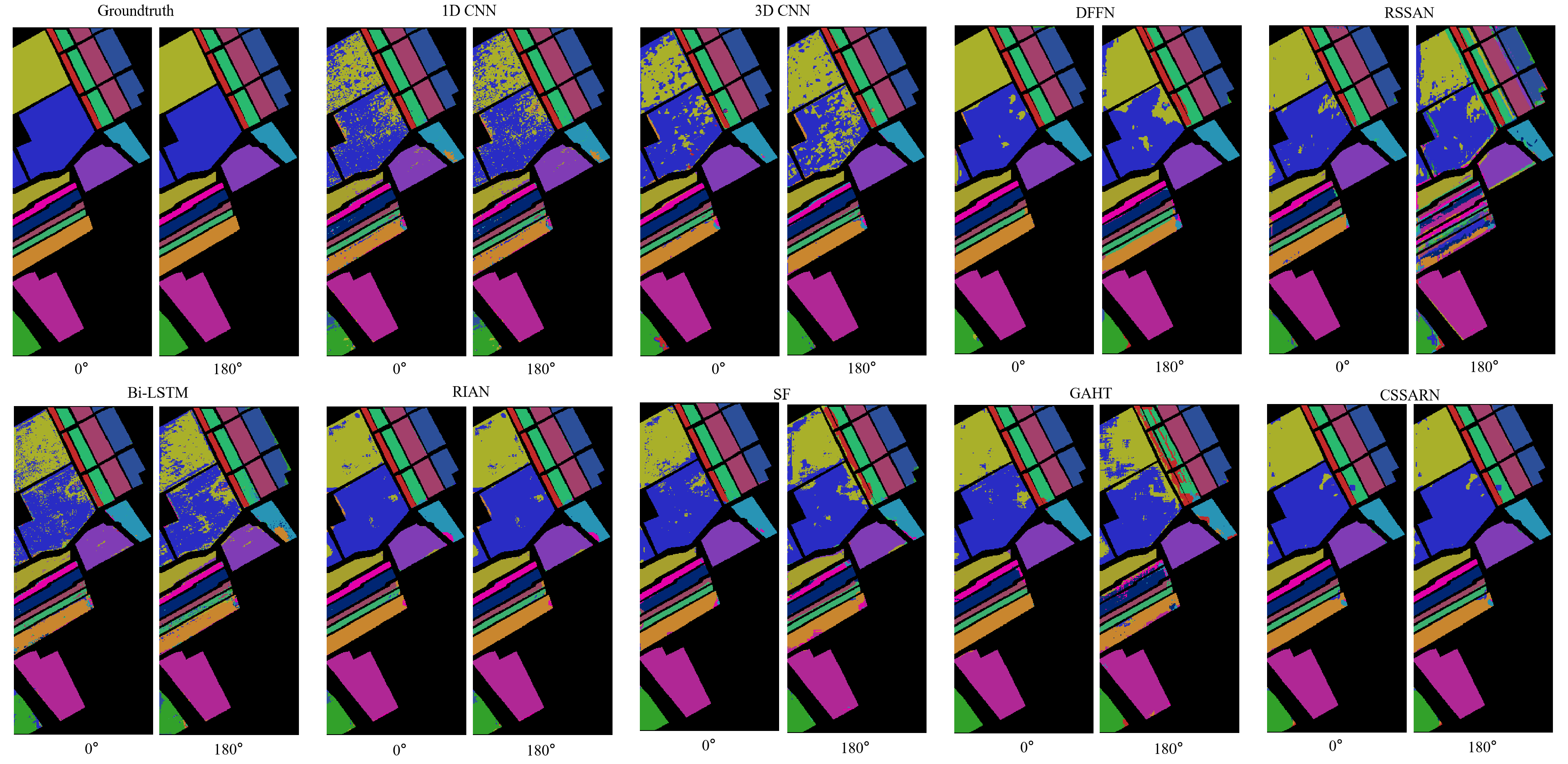
- Indian Pines: Table 7 and Table 8 show the OA, AA, and Kappa coefficients corresponding to 0° and 180° for each algorithm on the IP dataset in detail. Fifteen categories of 3D CNN show a decrease in accuracy. Class 1 “Alfalfa” and Class 9 “Oats” have significant decreases in accuracy. This indicates that 3D CNN cannot learn the features of these samples, resulting in a decrease in accuracy. The performance results of the DFFN and the RSSAN are similar to that of 3D CNN. The accuracy is dropped in all categories. This means that these algorithms generalize poorly to new datasets. The Bi-LSTM shows a decrease in the accuracy of 15 classes. The classification accuracy of Class 3 “Corn-Mintill”, Class 12 “Soybean-Clean”, and Class 15 “Buildings-Grass-Trees-Drives” is dropped by more than 40%. The training samples for these classes are sufficient. It may be that the network learns spatial features that are unimportant for these classes and does not maintain good generalization when there is a change in land cover distribution. The performance of 1D CNN and RIAN on the dataset before and after rotation does not change; this is because both use 1 × 1 convolutional kernels and the features do not change with image rotation.
Table 7. Category accuracy, OA(%), AA(%), and for each method at 0° degrees on the IP dataset.
Table 8. Category accuracy, OA(%), AA(%), and for each method at 180° degrees on the IP dataset.Transformer-based algorithms appear less effective than CNN-based algorithms when confronted with differences in land cover distribution variations due to spatial rotation. The classification accuracy of the SF is declined in all 16 categories, with more than 40% declines in Class 1 “Alfalfa”, Class 3 “Corn-Mintill”, Class 4 “Corn”, Class 5 “Grass-Pasture”, Class 7 “Grass-Pasture-Mowed”, Class 9 “Oats”, and Class 12 “Soybean-Clean”. This indicates that SF is unable to learn its discriminative features when faced with small samples. Instead, it focuses on its subtle spatial features when confronted with more adequate training samples, leading to its category misclassification when confronted with changes in land cover distribution due to spatial rotation. The performance of the GAHT is similar to that of SF.The proposed CSSARN in this paper achieves the best results in OA, AA, and Kappa values. The OA, AA, and Kappa values of the neural network algorithms based on spectral–spatial features are all significantly decreased when tested on the new dataset. In the meantime, the proposed CSSARN could have better generalization to spatial rotation.Figure 13 shows the visualization of each algorithm on the IP dataset. To facilitate the comparison with the 0° image, the 180° image is rotated in this paper, which can provide a more intuitive feel for the differences in classification errors caused by different algorithms due to rotation. The proposed CSSARN in this paper has the best visualization.
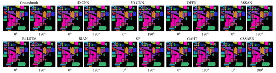 Figure 13. The visualization of each method on the IP dataset.
 - 2.
- Salinas: Table 9 and Table 10 list the OA, AA, and Kappa coefficients for each algorithm on the SA dataset. The performance of 1D CNN and RIAN remains unaffected by rotation, while all the remaining spectral–spatial-based neural network methods show a decrease in accuracy. Compared to the IP dataset, the comparative methods show a smaller decrease. This may be because the spatial resolution of the SA dataset is higher than that of the IP dataset. The CSSARN achieves the best classification accuracy on the original dataset in 9 categories. And on the rotated new dataset, the CSSARN achieves the best classification accuracy in 12 categories. It demonstrates the excellent generalization ability of our algorithm.
Table 9. Category accuracy, OA(%), AA(%), and for each method at 0° degrees on the SA dataset.
Table 10. Category accuracy, OA(%), AA(%), and for each method at 180° degrees on the SA dataset.Figure 14 shows the visualization of each method on the SA dataset. Similar to the IP dataset, the 180° image is rotated in this paper to facilitate the comparison with the 0° image. At the same time, the proposed CSSARN has the best visualization.
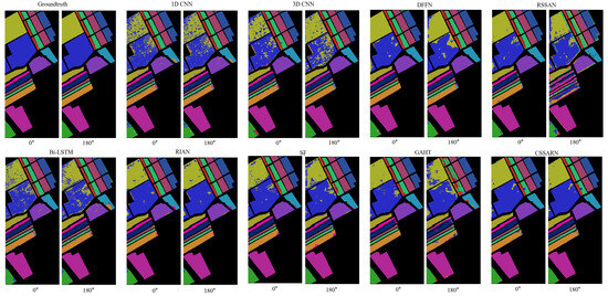 Figure 14. The visualization of each method on the SA dataset.
 - 3.
- Data Augmentation: Table 11 lists the OA for each algorithm, without or with data augmentation, on the IP and SA datasets. As both 1D CNN and RIAN utilize 1 × 1 convolutional kernels, their performance is not affected by rotation. After data augmentation, the performance of all methods on the original and rotated datasets is significantly improved, particularly on the rotated dataset. For the IP dataset, data augmentation enhances the Transformer-based approach most significantly. After data augmentation, the OAs of SF and GAHT are improved by 21.68% and 19.52%, respectively, on the rotated dataset. For the SA dataset, data augmentation improves RSSAN the most on the rotated dataset, with an OA improvement of 9.05%. This means that data augmentation can alleviate the problem of decreasing classification accuracy due to the difference in feature distribution caused by rotation. However, even after using the data augmentation method, there is still a significant accuracy decrease on the rotated dataset. This indicates that data augmentation by rotation still cannot make the algorithm effectively cope with the problem of different feature distributions due to rotation.
Table 11. OA(%) for each method, with or without data augmentation, on the IP and the SA datasets.The accuracy of the proposed CSSARN is further improved after data augmentation, and the best OA is achieved. In addition, CSSARN shows no accuracy degradation on the rotated dataset, which suggests that the proposed method can more effectively cope with the problem of different feature distributions due to rotation.
- 4.
- GF14-C17: Table 12 displays the OA, AA, and kappa values of the methods on GF14-C17. The DFFN achieves the best classification accuracy in Class 1 “Cabbage”, Class 3 “Scallion”, Class 5 “Cole Flower”, Class 6 “Corn”, Class 11 “Pit-Pond”, Class 15 “Privet Tree” and Class 16 “Pear Tree”. The CSSARN does not differ much from DFFN in these categories. The most significant difference is in Class 16 “Pear Tree”, with a difference of about 13.77%. The CSSARN does not consider the sample imbalance problem, so the extracted features of small samples may be lost as the network depth deepens. The best classification accuracy of Class 2 “Potato”, Class 12 “Greenhouse”, and Class 17 “Purple Leaf Plum” is achieved by the GAHT. The CSSARN is 7.06% lower than the GAHT on Class 16 “Pear Tree”. Because the training samples for this category are small, the CSSARN loses features from small samples when extracting spatial features, resulting in poor performance on small samples.
Table 12. Category accuracy, OA(%), AA(%), and for each method on the GF14-C17 dataset.Although the CSSARN attains the best classification accuracy for only seven categories, the OA, the AA, and the Kappa values are the highest. This indicates that the CSSARN performs less well than a particular method in some categories but has a better overall performance. The OA is improved by at least 1.02% on GF14-C17.Figure 15 illustrates the visualization of each algorithm on GF14-C17. Considering that the original image is large, only the image containing the test sample region is shown here, and the whole image is not. From the visualization results, the difference between the CSSARN and the ground truth is not apparent, while the other algorithms have noticeable differences with the ground truth. It indicates that the CSSARN could effectively learn spectral–spatial features and achieve high classification accuracy.
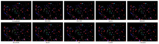 Figure 15. The visualization of each method on the GF14-C17 dataset.
 - 5.
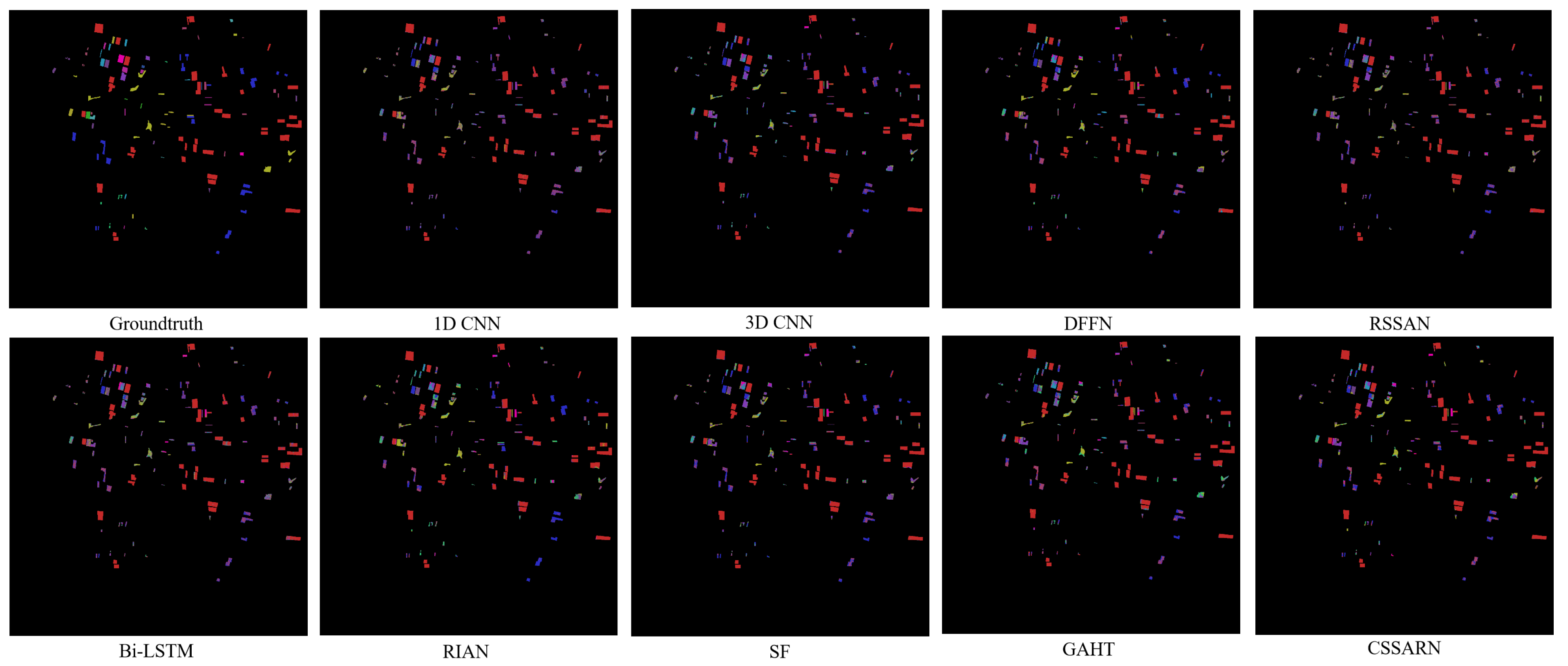
- GF14-C16: The training samples are selected in GF14-C17 and tested on GF14-C16, which can avoid the problem caused by randomly dividing training/testing samples on the same dataset completely. The categories included in GF14-C17 are also all present in GF14-C16 without considering the spectral differences and category differences, and the generalization of the algorithm can be verified well.The OA, AA, and kappa values of the method on GF14-C16 are listed in Table 13. The DFFN achieves the best classification accuracy in Class 1 “Cabbage”. The CSSARN does not differ much from the DFFN in this category. Transformer-based methods SF and GAHT realize the best classification accuracies on Class 6 “Corn” only. The difference in the classification accuracy of CNN-based methods in this category is insignificant. The Bi-LSTM achieves the best classification accuracy in Class 10 “Onions” but only 31.31%. This indicates that the difference in the spatial distribution of this category in the two images is significant, leading to poor performance for most algorithms. Meanwhile, the Bi-LSTM outperforms the CSSARN by 36.58% in Class 12 “Greenhouse”. This means that the CSSARN has over 20 sample errors in this category. This indicates that CSSARN focuses too much on the spectral–spatial features of the original training set in this category, which in turn performs poorly when tested for generalizability. RIAN achieves the best accuracy in Class 5 “Cole Flower”, Class 8 “Peanut” and Class 11 “Pit-Pond”. It also achieves sub-optimal performance on the OA, AA, and Kappa metrics and significantly outperforms other methods. This may be attributed to its design to cope with spatial variations.
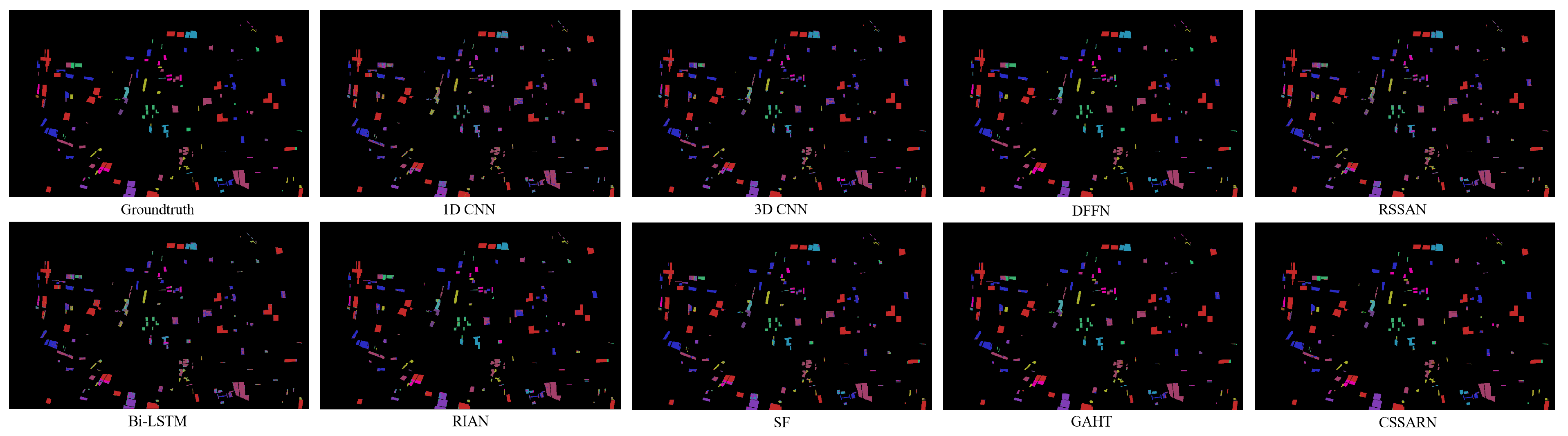
Table 13. Category accuracy, OA(%), AA(%), and for each method on the GF14-C16 dataset.It is worth noting that all the algorithms perform poorly in Class 7 “Chinese Cabbage”, Class 14 “Peach Tree”, and Class 17 “Purple Leaf Plum”, indicating that the spatial distributions of these classes in the new scene are completely different from those of the original training set. Therefore, the method based on spectral–spatial features fails in these categories. The failure of the spectral feature-based method in these categories is probably due to the overfitting problem caused by the “same class with different spectra”, which pays too much attention to the spectral features of the training set, resulting in poor generalization.Although the CSSARN attains the best classification accuracy for only seven categories, the OA, the AA, and the Kappa values are the highest. The OA is improved by at least 3.49% on GF14-C16. This also shows the better generalization of the CSSARN compared to other algorithms.Figure 16 displays the classification visualization of each algorithm on GF14-C16. It can be seen that the CSSARN is closer to the ground truth. This shows that CSSARN could learn spectral–spatial features efficiently and achieve good classification accuracy in generalizability tests.
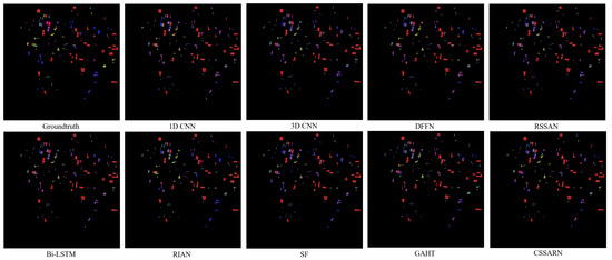 Figure 16. The visualization of each method on the GF14-C16 dataset.
5. Discussion
Figure 13, Figure 14, Figure 15 and Figure 16 show the classification visualization results of different methods on different datasets. Table 7, Table 8, Table 9, Table 10, Table 11, Table 12 and Table 13 show in detail the classification accuracy, average accuracy (AA), overall accuracy (OA), and Kappa coefficient () of these algorithms for each category on different datasets. Specifically, CSSARN maintains good generalization even with the rotated dataset, while the classification accuracy of all other spectral–spatial methods decreases significantly. Based on this analysis, the number of parameters and time efficiency of the model are explored in this section.
As can be seen from Table 14, the average number of parameters of CSSARN is the least, only 0.02 M, which is much lower than other methods. This indicates that CSSARN effectively compresses the number of network parameters while maintaining classification accuracy, which could achieve higher classification accuracy with fewer parameters. It also shows that the parameters of many existing algorithms are redundant.
Table 14.
The number of parameters for each algorithm on the different datasets.
Table 15 lists the training and testing times for each method. The 1D CNN and 3D CNN have the lowest training time and testing times in all datasets, indicating that these algorithms are the most time efficient. Even though the proposed algorithm has the least number of parameters, its training and testing times are longer compared to 1D CNN, which is mainly because the dynamic convolutional training process consumes a longer time. In contrast, the training and testing times of CSSARN are within a reasonably acceptable range.
Table 15.
Training and testing times of each method on different datasets.
6. Conclusions
This paper summarizes the problem caused by single-scene datasets in deep learning-based hyperspectral image classification. Two new methods are proposed to alleviate the above issues. The first method is to rotate the original image. The second method is to construct a new cross-scene dataset. Based on this, a constrained spectral–spatial attention residual network is proposed. This network mainly contains a spectral feature learning module, a spatial feature learning module, and a feature fusion module. Specifically, the spectral feature learning module includes a constrained spectral attention mechanism and a spectral feature extraction module. The constrained spectral attention module uses spectral angle mapping to generate adaptive spectral attention weights, which reduces interference between different categories. Then, the spectral features are extracted by a spectral feature extraction module constructed from residual blocks. At the same time, the spatial feature learning module includes a constrained spatial attention mechanism and a spatial feature extraction module. Constrained spatial attention uses a pyramidal approach to obtain different spatial weights. The spatial features are then extracted by a spatial feature extraction module constructed from the residual block consisting of dynamic convolution. Finally, the spectral and spatial features are fused and fed into the classifier to complete the classification.
The most important point is that this paper proposes a new cross-scene dataset GF14-C17&C16. The proposed dataset could avoid the problem caused by randomly dividing training/testing samples on the same dataset and could objectively evaluate the generalization of the algorithm. Extensive experiments on two publicly available hyperspectral datasets and the GF14 dataset have demonstrated the superior performance of CSSARN in extracting spectral and spatial features more efficiently than other methods.
However, it is important to note that when tested on new cross-scene datasets, the results do not achieve satisfactory classification accuracy. Future research will focus on improving classification accuracy for cross-scene datasets.
Author Contributions
Conceptualization, S.L. and Y.S.; Data curation, S.L. and G.Z.; Formal analysis, S.L., B.C. and Y.S.; Funding acquisition, S.L., G.Z. and J.L.; Investigation, S.L. and B.C.; Methodology, S.L. and Y.S.; Project administration, S.L., G.Z. and J.L.; Resources, S.L. and B.C.; Software, S.L. and Y.S.; Supervision, S.L. and G.Z.; Validation, S.L., N.W., Y.S. and J.L.; Visualization, S.L., B.C. and G.Z.; Writing—original draft, S.L., Y.S. and J.L.; Writing—review and editing, S.L., G.Z. and J.L. All authors have read and agreed to the published version of the manuscript.
Funding
This research was supported in part by the National Natural Science Foundation of China under Grant 42176182, in part by the National Science Basic Research Foundation of Shaanxi Province under Grant 2023-YBGY-390, in part by the State Key Laboratory of Tropical Oceanography, South China Sea Institute of Oceanology, Chinese Academy of Sciences (Project No. LTO2206), and in part by the Public Fund of the State Key Laboratory of Satellite Ocean Environment Dynamics, Second Institute of Oceanography, Ministry of Natural Resources, under Grant QNHX3126.
Data Availability Statement
Data are available in a publicly accessible repository that does not issue DOIs. Publicly available datasets were analyzed in this study. These data can be found here: Indian Pines and Salinas: http://www.ehu.eus/ccwintco/index.php?title=Hyperspectral_Remote_Sensing_Scenes (accessed on 16 June 2022), and GF14-C17&C16: https://github.com/ChillLingo/GF14-C17C16 (accessed on 21 June 2024). All data used in this paper can also be obtained by contacting the first or corresponding author.
Conflicts of Interest
The authors declare that the research was conducted in the absence of any commercial or financial relationships that could be construed as potential conflicts of interest.
References
- Zhang, L.; Zhang, L. Artificial intelligence for remote sensing data analysis: A review of challenges and opportunities. IEEE Geosci. Remote Sens. Mag. 2022, 10, 270–294. [Google Scholar] [CrossRef]
- Crowson, M.; Hagensieker, R.; Waske, B. Mapping land cover change in northern Brazil with limited training data. Int. J. Appl. Earth Obs. Geoinf. 2019, 78, 202–214. [Google Scholar] [CrossRef]
- Wang, N.; Shi, Y.; Li, H.; Zhang, G.; Li, S.; Liu, X. Multi-Prior Graph Autoencoder with Ranking-Based Band Selection for Hyperspectral Anomaly Detection. Remote Sens. 2023, 15, 4430. [Google Scholar] [CrossRef]
- Shi, Y.; Wang, N.; Yang, F.; Zhang, G.; Li, S.; Liu, X. Multispectral Images Deblurring via Interchannel Correlation Relationship. In Proceedings of the 2021 4th International Conference on Information Communication and Signal Processing (ICICSP), Shanghai, China, 24–26 September 2021; IEEE: Piscataway, NJ, USA, 2021; pp. 458–462. [Google Scholar]
- Nguyen, C.; Sagan, V.; Maimaitiyiming, M.; Maimaitijiang, M.; Bhadra, S.; Kwasniewski, M.T. Early Detection of Plant Viral Disease Using Hyperspectral Imaging and Deep Learning. Sensors 2021, 21, 742. [Google Scholar] [CrossRef] [PubMed]
- Fang, J.; Yuan, Y.; Lu, X.; Feng, Y. Robust space–frequency joint representation for remote sensing image scene classification. IEEE Trans. Geosci. Remote Sens. 2019, 57, 7492–7502. [Google Scholar] [CrossRef]
- Ahmad, M.; Shabbir, S.; Roy, S.K.; Hong, D.; Wu, X.; Yao, J.; Khan, A.M.; Mazzara, M.; Distefano, S.; Chanussot, J. Hyperspectral image classification—Traditional to deep models: A survey for future prospects. IEEE J. Sel. Top. Appl. Earth Obs. Remote Sens. 2021, 15, 968–999. [Google Scholar] [CrossRef]
- Singh, S.; Kasana, S.S. A Pre-processing framework for spectral classification of hyperspectral images. Multimed. Tools Appl. 2021, 80, 243–261. [Google Scholar] [CrossRef]
- Manifold, B.; Men, S.; Hu, R.; Fu, D. A versatile deep learning architecture for classification and label-free prediction of hyperspectral images. Nat. Mach. Intell. 2021, 3, 306–315. [Google Scholar] [CrossRef]
- Roy, S.K.; Krishna, G.; Dubey, S.R.; Chaudhuri, B.B. HybridSN: Exploring 3-D–2-D CNN feature hierarchy for hyperspectral image classification. IEEE Geosci. Remote Sens. Lett. 2019, 17, 277–281. [Google Scholar] [CrossRef]
- Wei, W.; Song, C.; Zhang, L.; Zhang, Y. Lightweighted hyperspectral image classification network by progressive bi-quantization. IEEE Trans. Geosci. Remote Sens. 2023, 61, 1–14. [Google Scholar] [CrossRef]
- Feng, H.; Wang, Y.; Li, Z.; Zhang, N.; Zhang, Y.; Gao, Y. Information leakage in deep learning-based hyperspectral image classification: A survey. Remote Sens. 2023, 15, 3793. [Google Scholar] [CrossRef]
- Li, J.; Huang, X.; Tu, L. WHU-OHS: A benchmark dataset for large-scale Hersepctral Image classification. Int. J. Appl. Earth Obs. Geoinf. 2022, 113, 103022. [Google Scholar] [CrossRef]
- Audebert, N.; Le Saux, B.; Lefevre, S. Deep Learning for Classification of Hyperspectral Data: A Comparative Review. IEEE Geosci. Remote Sens. Mag. 2019, 7, 159–173. [Google Scholar] [CrossRef]
- Sun, H.; Zheng, X.; Lu, X. A supervised segmentation network for hyperspectral image classification. IEEE Trans. Image Process. 2021, 30, 2810–2825. [Google Scholar] [CrossRef] [PubMed]
- Tobler, W.R. A Computer Movie Simulating Urban Growth in the Detroit Region. Econ. Geogr. 1970, 46, 234–240. [Google Scholar] [CrossRef]
- Liang, J.; Zhou, J.; Qian, Y.; Wen, L.; Bai, X.; Gao, Y. On the sampling strategy for evaluation of spectral-spatial methods in hyperspectral image classification. IEEE Trans. Geosci. Remote Sens. 2016, 55, 862–880. [Google Scholar] [CrossRef]
- Li, G.; Ma, S.; Li, K.; Zhou, M.; Lin, L. Band selection for heterogeneity classification of hyperspectral transmission images based on multi-criteria ranking. Infrared Phys. Technol. 2022, 125, 104317. [Google Scholar] [CrossRef]
- Moharram, M.A.; Sundaram, D.M. Dimensionality reduction strategies for land use land cover classification based on airborne hyperspectral imagery: A survey. Environ. Sci. Pollut. Res. 2023, 30, 5580–5602. [Google Scholar] [CrossRef]
- Gewali, U.B.; Monteiro, S.T.; Saber, E. Machine learning based hyperspectral image analysis: A survey. arXiv 2018, arXiv:1802.08701. [Google Scholar]
- Zhong, C.; Zhang, J.; Wu, S.; Zhang, Y. Cross-Scene Deep Transfer Learning With Spectral Feature Adaptation for Hyperspectral Image Classification. IEEE J. Sel. Top. Appl. Earth Obs. Remote Sens. 2020, 13, 2861–2873. [Google Scholar] [CrossRef]
- Samat, A.; Gamba, P.; Abuduwaili, J.; Liu, S.; Miao, Z. Geodesic Flow Kernel Support Vector Machine for Hyperspectral Image Classification by Unsupervised Subspace Feature Transfer. Remote Sens. 2016, 8, 234. [Google Scholar] [CrossRef]
- Shen, J.; Cao, X.; Li, Y.; Xu, D. Feature Adaptation and Augmentation for Cross-Scene Hyperspectral Image Classification. IEEE Geosci. Remote Sens. Lett. 2018, 15, 622–626. [Google Scholar] [CrossRef]
- Zhang, Y.; Li, W.; Zhang, M.; Qu, Y.; Tao, R.; Qi, H. Topological Structure and Semantic Information Transfer Network for Cross-Scene Hyperspectral Image Classification. IEEE Trans. Neural Networks Learn. Syst. 2023, 34, 2817–2830. [Google Scholar] [CrossRef] [PubMed]
- Zhang, Y.; Li, W.; Sun, W.; Tao, R.; Du, Q. Single-Source Domain Expansion Network for Cross-Scene Hyperspectral Image Classification. IEEE Trans. Image Process. 2023, 32, 1498–1512. [Google Scholar] [CrossRef] [PubMed]
- Zheng, X.; Sun, H.; Lu, X.; Xie, W. Rotation-invariant attention network for hyperspectral image classification. IEEE Trans. Image Process. 2022, 31, 4251–4265. [Google Scholar] [CrossRef] [PubMed]
- Melgani, F.; Bruzzone, L. Classification of hyperspectral remote sensing images with support vector machines. IEEE Trans. Geosci. Remote Sens. 2004, 42, 1778–1790. [Google Scholar] [CrossRef]
- Gomez-Chova, L.; Calpe, J.; Soria, E.; Camps-Valls, G.; Martin, J.; Moreno, J. CART-based feature selection of hyperspectral images for crop cover classification. In Proceedings of the 2003 International Conference on Image Processing (Cat. No.03CH37429), Barcelona, Spain, 14–17 September 2003; Volume 3, p. III-589. [Google Scholar]
- Ham, J.; Chen, Y.; Crawford, M.M.; Ghosh, J. Investigation of the random forest framework for classification of hyperspectral data. IEEE Trans. Geosci. Remote Sens. 2005, 43, 492–501. [Google Scholar] [CrossRef]
- Liu, X.; Hu, Q.; Cai, Y.; Cai, Z. Extreme learning machine-based ensemble transfer learning for hyperspectral image classification. IEEE J. Sel. Top. Appl. Earth Obs. Remote Sens. 2020, 13, 3892–3902. [Google Scholar] [CrossRef]
- Li, S.; Song, W.; Fang, L.; Chen, Y.; Ghamisi, P.; Benediktsson, J.A. Deep learning for hyperspectral image classification: An overview. IEEE Trans. Geosci. Remote Sens. 2019, 57, 6690–6709. [Google Scholar] [CrossRef]
- Paoletti, M.E.; Haut, J.M.; Fernandez-Beltran, R.; Plaza, J.; Plaza, A.J.; Pla, F. Deep pyramidal residual networks for spectral–spatial hyperspectral image classification. IEEE Trans. Geosci. Remote Sens. 2018, 57, 740–754. [Google Scholar] [CrossRef]
- Yang, X.; Ye, Y.; Li, X.; Lau, R.Y.; Zhang, X.; Huang, X. Hyperspectral image classification with deep learning models. IEEE Trans. Geosci. Remote Sens. 2018, 56, 5408–5423. [Google Scholar] [CrossRef]
- Hu, W.; Huang, Y.; Wei, L.; Zhang, F.; Li, H. Deep convolutional neural networks for hyperspectral image classification. J. Sensors 2015, 2015, 258619. [Google Scholar] [CrossRef]
- Chen, Y.; Lin, Z.; Zhao, X.; Wang, G.; Gu, Y. Deep learning-based classification of hyperspectral data. IEEE J. Sel. Top. Appl. Earth Obs. Remote Sens. 2014, 7, 2094–2107. [Google Scholar] [CrossRef]
- Paoletti, M.E.; Haut, J.M.; Plaza, J.; Plaza, A. Deep learning classifiers for hyperspectral imaging: A review. ISPRS J. Photogramm. Remote Sens. 2019, 158, 279–317. [Google Scholar] [CrossRef]
- Yu, S.; Jia, S.; Xu, C. Convolutional neural networks for hyperspectral image classification. Neurocomputing 2017, 219, 88–98. [Google Scholar] [CrossRef]
- Mou, L.; Ghamisi, P.; Zhu, X.X. Deep recurrent neural networks for hyperspectral image classification. IEEE Trans. Geosci. Remote Sens. 2017, 55, 3639–3655. [Google Scholar] [CrossRef]
- Wu, H.; Prasad, S. Convolutional recurrent neural networks for hyperspectral data classification. Remote Sens. 2017, 9, 298. [Google Scholar] [CrossRef]
- Wambugu, N.; Chen, Y.; Xiao, Z.; Tan, K.; Wei, M.; Liu, X.; Li, J. Hyperspectral image classification on insufficient-sample and feature learning using deep neural networks: A review. Int. J. Appl. Earth Obs. Geoinf. 2021, 105, 102603. [Google Scholar] [CrossRef]
- Li, J.; Zhao, X.; Li, Y.; Du, Q.; Xi, B.; Hu, J. Classification of hyperspectral imagery using a new fully convolutional neural network. IEEE Geosci. Remote Sens. Lett. 2018, 15, 292–296. [Google Scholar] [CrossRef]
- Haut, J.M.; Paoletti, M.E.; Plaza, J.; Plaza, A.; Li, J. Hyperspectral image classification using random occlusion data augmentation. IEEE Geosci. Remote Sens. Lett. 2019, 16, 1751–1755. [Google Scholar] [CrossRef]
- Xu, Y.; Du, B.; Zhang, F.; Zhang, L. Hyperspectral image classification via a random patches network. ISPRS J. Photogramm. Remote Sens. 2018, 142, 344–357. [Google Scholar] [CrossRef]
- Bera, S.; Shrivastava, V.K.; Satapathy, S.C. Advances in Hyperspectral Image Classification Based on Convolutional Neural Networks: A Review. Comput. Model. Eng. Sci. 2022, 133, 219–250. [Google Scholar] [CrossRef]
- Ghamisi, P.; Maggiori, E.; Li, S.; Souza, R.; Tarablaka, Y.; Moser, G.; De Giorgi, A.; Fang, L.; Chen, Y.; Chi, M.; et al. New frontiers in spectral-spatial hyperspectral image classification: The latest advances based on mathematical morphology, Markov random fields, segmentation, sparse representation, and deep learning. IEEE Geosci. Remote Sens. Mag. 2018, 6, 10–43. [Google Scholar] [CrossRef]
- Liu, H.; Li, W.; Xia, X.G.; Zhang, M.; Gao, C.Z.; Tao, R. Central attention network for hyperspectral imagery classification. IEEE Trans. Neural Netw. Learn. Syst. 2022, 34, 8989–9003. [Google Scholar] [CrossRef] [PubMed]
- Lei, S.; Shi, Z.; Zou, Z. Coupled Adversarial Training for Remote Sensing Image Super-Resolution. IEEE Trans. Geosci. Remote Sens. 2020, 58, 3633–3643. [Google Scholar] [CrossRef]
- Mei, S.; Ji, J.; Geng, Y.; Zhang, Z.; Li, X.; Du, Q. Unsupervised spatial–spectral feature learning by 3D convolutional autoencoder for hyperspectral classification. IEEE Trans. Geosci. Remote Sens. 2019, 57, 6808–6820. [Google Scholar] [CrossRef]
- Dosovitskiy, A.; Beyer, L.; Kolesnikov, A.; Weissenborn, D.; Zhai, X.; Unterthiner, T.; Dehghani, M.; Minderer, M.; Heigold, G.; Gelly, S.; et al. An image is worth 16x16 words: Transformers for image recognition at scale. arXiv 2020, arXiv:2010.11929. [Google Scholar]
- He, J.; Zhao, L.; Yang, H.; Zhang, M.; Li, W. HSI-BERT: Hyperspectral image classification using the bidirectional encoder representation from transformers. IEEE Trans. Geosci. Remote Sens. 2019, 58, 165–178. [Google Scholar] [CrossRef]
- Zhong, Z.; Li, Y.; Ma, L.; Li, J.; Zheng, W.S. Spectral–spatial transformer network for hyperspectral image classification: A factorized architecture search framework. IEEE Trans. Geosci. Remote Sens. 2021, 60, 1–15. [Google Scholar] [CrossRef]
- Roy, S.K.; Deria, A.; Shah, C.; Haut, J.M.; Du, Q.; Plaza, A. Spectral–Spatial Morphological Attention Transformer for Hyperspectral Image Classification. IEEE Trans. Geosci. Remote Sens. 2023, 61, 1–15. [Google Scholar] [CrossRef]
- Moharram, M.A.; Sundaram, D.M. Land use and land cover classification with hyperspectral data: A comprehensive review of methods, challenges and future directions. Neurocomputing 2023, 536, 90–113. [Google Scholar] [CrossRef]
- Shi, Y.; Fu, B.; Wang, N.; Cheng, Y.; Fang, J.; Liu, X.; Zhang, G. Spectral-Spatial Attention Rotation-Invariant Classification Network for Airborne Hyperspectral Images. Drones 2023, 7, 240. [Google Scholar] [CrossRef]
- Zhan, Y.; Wu, K.; Dong, Y. Enhanced Spectral–Spatial Residual Attention Network for Hyperspectral Image Classification. IEEE J. Sel. Top. Appl. Earth Obs. Remote Sens. 2022, 15, 7171–7186. [Google Scholar] [CrossRef]
- Wang, Y.; Song, T.; Xie, Y.; Roy, S.K. A probabilistic neighbourhood pooling-based attention network for hyperspectral image classification. Remote Sens. Lett. 2022, 13, 65–75. [Google Scholar]
- Liu, B.; Yu, A.; Gao, K.; Tan, X.; Sun, Y.; Yu, X. DSS-TRM: Deep spatial–spectral transformer for hyperspectral image classification. Eur. J. Remote Sens. 2022, 55, 103–114. [Google Scholar] [CrossRef]
- Lu, Z.; Xu, B.; Sun, L.; Zhan, T.; Tang, S. 3-D channel and spatial attention based multiscale spatial–spectral residual network for hyperspectral image classification. IEEE J. Sel. Top. Appl. Earth Obs. Remote Sens. 2020, 13, 4311–4324. [Google Scholar] [CrossRef]
- Zhang, X.; Shang, S.; Tang, X.; Feng, J.; Jiao, L. Spectral partitioning residual network with spatial attention mechanism for hyperspectral image classification. IEEE Trans. Geosci. Remote Sens. 2021, 60, 1–14. [Google Scholar] [CrossRef]
- Mei, S.; Li, X.; Liu, X.; Cai, H.; Du, Q. Hyperspectral image classification using attention-based bidirectional long short-term memory network. IEEE Trans. Geosci. Remote Sens. 2021, 60, 1–12. [Google Scholar]
- Shi, Y.; Fu, B.; Wang, N.; Chen, Y.; Fang, J. Multispectral Image Quality Improvement Based on Global Iterative Fusion Constrained by Meteorological Factors. Cogn. Comput. 2023, 16, 404–424. [Google Scholar] [CrossRef]
- Veit, A.; Wilber, M.J.; Belongie, S. Residual networks behave like ensembles of relatively shallow networks. In Advances in Neural Information Processing Systems; Curran Associates, Inc.: New York, NY, USA, 2016; Volume 29. [Google Scholar]
- Huang, G.; Liu, Z.; Van Der Maaten, L.; Weinberger, K.Q. Densely connected convolutional networks. In Proceedings of the IEEE Conference on Computer Vision and Pattern Recognition, Honolulu, HI, USA, 21–26 July 2017; pp. 4700–4708. [Google Scholar]
- Yang, B.; Bender, G.; Le, Q.V.; Ngiam, J. Condconv: Conditionally parameterized convolutions for efficient inference. In Advances in Neural Information Processing Systems; Curran Associates, Inc.: New York, NY, USA, 2019; Volume 32. [Google Scholar]
- Li, C.; Zhou, A.; Yao, A. Omni-dimensional dynamic convolution. arXiv 2022, arXiv:2209.07947. [Google Scholar]
- Chen, Y.; Dai, X.; Liu, M.; Chen, D.; Yuan, L.; Liu, Z. Dynamic convolution: Attention over convolution kernels. In Proceedings of the IEEE/CVF Conference on Computer Vision and Pattern Recognition, Seattle, WA, USA, 14–19 June 2020; pp. 11030–11039. [Google Scholar]
- Sun, H.; Li, Q.; Yu, J.; Zhou, D.; Chen, W.; Zheng, X.; Lu, X. Deep feature reconstruction learning for open-set classification of remote sensing imagery. IEEE Geosci. Remote. Sens. Lett. 2023, 20, 1–5. [Google Scholar] [CrossRef]
- Mei, S.; Song, C.; Ma, M.; Xu, F. Hyperspectral image classification using group-aware hierarchical transformer. IEEE Trans. Geosci. Remote Sens. 2022, 60, 1–14. [Google Scholar] [CrossRef]
- Li, Y.; Zhang, H.; Shen, Q. Spectral–spatial classification of hyperspectral imagery with 3D convolutional neural network. Remote Sens. 2017, 9, 67. [Google Scholar] [CrossRef]
- Song, W.; Li, S.; Fang, L.; Lu, T. Hyperspectral image classification with deep feature fusion network. IEEE Trans. Geosci. Remote Sens. 2018, 56, 3173–3184. [Google Scholar] [CrossRef]
- Zhu, M.; Jiao, L.; Liu, F.; Yang, S.; Wang, J. Residual spectral–spatial attention network for hyperspectral image classification. IEEE Trans. Geosci. Remote Sens. 2020, 59, 449–462. [Google Scholar] [CrossRef]
- Hong, D.; Han, Z.; Yao, J.; Gao, L.; Zhang, B.; Plaza, A.; Chanussot, J. SpectralFormer: Rethinking hyperspectral image classification with transformers. IEEE Trans. Geosci. Remote Sens. 2021, 60, 1–15. [Google Scholar] [CrossRef]


Disclaimer/Publisher’s Note: The statements, opinions and data contained in all publications are solely those of the individual author(s) and contributor(s) and not of MDPI and/or the editor(s). MDPI and/or the editor(s) disclaim responsibility for any injury to people or property resulting from any ideas, methods, instructions or products referred to in the content. |
© 2024 by the authors. Licensee MDPI, Basel, Switzerland. This article is an open access article distributed under the terms and conditions of the Creative Commons Attribution (CC BY) license (https://creativecommons.org/licenses/by/4.0/).