Abstract
Stochastic optimization approaches benefit from random variance to produce a solution in a reasonable time frame that is good enough for solving the problem. Compared with them, deterministic optimization methods feature faster convergence rates and better reproducibility but may get stuck at a local optimum that is insufficient to solve the problem. In this paper, we propose a group-based deterministic optimization method, which can efficiently achieve comparable performance to heuristic optimization algorithms, such as particle swarm optimization. Moreover, the weighted sum method (WSM) is employed to further improve our deterministic optimization method to be multi-objective optimization, making it able to seek a balance among multiple conflicting circuit performance metrics. With a case study of three common analog circuits tested for our optimization methodology, the experimental results demonstrate that our proposed method can more efficiently reach a better estimation of the Pareto front compared to NSGA-II, a well-known multi-objective optimization approach.
1. Introduction
In recent years, with the continuous development and innovation in the field of integrated circuit design, traditional manual circuit parameter tuning has become increasingly more difficult to meet emerging application requirements [1]. Therefore, there is great demand to optimize circuit parameters through electronic design automation (EDA) tools, which can largely liberate engineers from design constraints, improve design speed, and enhance circuit performances.
Circuit parameter optimization can generally be categorized into stochastic methods and deterministic methods based on algorithmic strategies [2]. The stochastic methods, inspired by natural phenomena, such as particle swarm optimization (PSO) [3], simulated annealing (SA) [4], evolutionary algorithms (EA) [5], genetic algorithms (GA) [6], Bayesian optimization (BO) [7], and others, have shown promising results that benefit from random variance. In contrast, deterministic optimization methods seek the optimal solution for circuit parameters by computing specific mathematical functions and equations, without utilizing random methods throughout the entire process [8]. In practical circuit design, using deterministic methods to optimize circuit parameters allows engineers to conduct repeated experiments on a circuit. Each experiment yields the same solution consistently, regardless of the number of repetitions. This facilitates engineers in finding a specific set of circuit parameter values that meet their requirements.
Based on the number of performance metrics to be optimized, circuit parameter optimization can be divided into single-objective optimization and multi-objective optimization [9]. Single-objective optimization focuses on optimizing a single performance of the circuit to obtain its extremum. In multi-objective optimization, the optimization of circuit parameters is not only aimed at a single circuit performance but also considers multiple circuit performances that may often have competing relationships. Compared to single-objective optimization, this is more challenging as it requires seeking a balance among multiple circuit performance metrics. In this scenario, we introduce the concept of Pareto optimality [10]. Pareto optimality refers to a state in multi-objective optimization problems where further optimization cannot be achieved by improving one objective without sacrificing others. If for a particular solution, none of the objectives can be improved without worsening others, then that solution is considered Pareto optimal. Pareto optimality emphasizes the need to balance trade-offs when facing conflicting objectives and to determine the best possible solution, making it a core concept in multi-objective optimization. The Pareto optimal front reflects the different optimization capabilities of the circuit when considering the trade-offs involved in multi-objective optimization. Obtaining the Pareto front solutions as accurately as possible is the primary objective of multi-objective optimization.
Reference [11] proposes a classical weighted sum method (WSM) to obtain the Pareto front. WSM involves multiplying each objective function by a weighting factor and then summing all the weighted objective functions together to transform multiple objective functions into an aggregated objective function. It systematically changes each weighting coefficient according to a certain pattern, with each different single objective optimization determining a different optimal solution to obtain the set of solutions on the Pareto front. Reference [12] applies the idea of multi-objective optimization to the design of analog integrated circuits and radio frequency integrated circuits, seeking Pareto design points among various circuit performance metrics. Reference [13] utilizes the NSGA-II [14] to obtain the Pareto solution set and applied it to the design of ring oscillators. Reference [15] proposes an efficient surrogate-assisted constrained multi-objective evolutionary algorithm for analog circuit sizing, which has been shown to achieve better results compared to the NSGA-II. As research advances, the application of multi-objective optimization methods in circuit parameter optimization has become increasingly sophisticated, and the algorithms for obtaining the Pareto front are continually improving.
However, up to now, using deterministic methods for multi-objective optimization of circuit parameters has not been fully investigated yet. Current research primarily uses deterministic methods to optimize circuit parameters for a single objective. It is challenging to avoid using random variance throughout the entire process of addressing multi-objective optimization, which would inevitably produce stochastic outcomes. In this paper, an innovation is made to an existing deterministic optimization algorithm to improve its efficiency and effectiveness, contributing to its ability to efficiently identify global optimal solutions for a single objective. Then, we integrate the WSM method and our deterministic optimization method together to realize deterministic multi-objective optimization, which would generate a deterministic Pareto front among various circuit performances. As our experimental results indicated, the Pareto front obtained by our method is superior in quality compared to that obtained by NSGA-II.
2. Proposed Methods
Starting from an initial set of circuit parameters, the deterministic optimization algorithm proposed in [16] utilizes the characteristic boundary curve (CBC) algorithm to determine the correction values for circuit parameters at each optimization iteration, continuously refining the circuit parameter values to converge towards the optimal solution. However, this method suffers from some limitations. Firstly, its optimization efficiency and effectiveness are poor when circuit biases are involved as parameters to be optimized since it is originally targeted at optimizing device sizes with fixed circuit biases provided. Secondly, it lacks means to let its optimized results escape from local optima, making it mostly converge to a local optimum. Thirdly, it can only optimize a single objective.
In this paper, we are motivated to propose a novel deterministic multi-objective optimization method, which has the following three features:
- (1)
- Boost the efficiency and effectiveness of single-objective deterministic optimization through our proposed various schemes;
- (2)
- Enhance the single-objective deterministic optimization to be able to derive global optimal solutions;
- (3)
- Improve the deterministic optimization from single-objective to be multiple-objective.
2.1. Design Parameter Classification and Correction
The key to deterministic optimization is to determine the parameter correction (i.e., parameter change) at each optimization iteration. In this paper, we propose a new method to calculate parameter correction.
Firstly, we classify the design parameters based on their types, including bias voltage, bias current, transistor length, transistor width, resistor, and capacitor. Then the parameter correction is calculated for each type (index of i) of design parameters via the modified generalized boundary curve (GBC) algorithm proposed in [17], which has the following objective function:
where represents the parameter correction of the ith type of design parameters, factor α is a positive constant for the scaling purpose, variable λ controls the weight of the squared Euclidean norm of , and is the linearized error of the ith type of design parameters:
where refers to the performance specification, is the performance gradients of current design parameter values (i.e., v) calculated by linearizing circuit performance f(v) at v (i.e., Equation (3)), and is the vector divided from that represents the performance gradients of the ith type of design parameters:
Compared with the original CBC algorithm used to derive parameter correction, the modified GBC algorithm features much higher efficiency and can address the issue when the cost function is strongly nonlinear [17]. Moreover, since different types of design parameters have distinct sensitivities to a parameter change, calculating the parameter correction of each type of design parameters rather than the whole design parameters ensures more smooth and accurate updating of design parameters during the iterative optimization process, making it possess much better optimization efficiency and effectiveness than the work of [16].
2.2. Bias-Aware Updating Scheme
Through our experimental studies, we have found that tuning the biases is more critical than adjusting device sizes when transistors work at improper regions, whose performance is usually far away from the specification. This observation has inspired us to bring forth the following bias-aware weight scheme, which can largely enhance the optimization efficacy:
- (1)
- When is applied:
- (2)
- When is applied:where and refer to the lower and upper bound performance requirements, respectively, a belongs to [0, 1), b is a natural number, and refer to the weights of the ith type of design parameters that are bias-type (e.g., bias voltage, bias current, or device sizes of any bias circuits) and other-type of design parameters, respectively.
At each optimization iteration, after deriving the parameter correction of each type of design parameters by following the instruction described in the last section, the proposed bias-aware weight scheme is applied to update the design parameter values as follows:
As one can see, when the current performance is quite distant from the specification, only bias-type design parameters can be tuned. Once it passes a certain threshold, both bias-type and other-type design parameters are adjusted simultaneously with distinct weights. Here, a and b are two crucial hyperparameters of our proposed group-based deterministic optimization algorithm. The hyperparameter a determines the region of circuit performance when only bias-type design parameters can be adjusted. In contrast, the hyperparameter b is used to decide the exact weights for bias-type and other-type design parameters when they can be tuned simultaneously. Specifically, a larger value of b would result in a more dramatic decrease and increase of weights for bias-type and other-type design parameters, respectively, as the circuit performance gets close to the target specification.
2.3. Group-Based Exploration Scheme
The deterministic optimization algorithm proposed in [16] can easily get stuck at a local optimum and has no means to jump out of it. In this paper, except for terminating condition (7), the terminating condition expressed in (8) is proposed to provide a chance for deterministic optimization to escape from local optima.
where µ is the index of optimization iteration. Condition (8) denotes that the performance can hardly be further improved in a successive user-defined (i.e., τ) number of optimization iterations while the improvement amount is controlled by a user-specified parameter δ.
However, although condition (8) can help deterministic optimization to escape from local optima to some extent, the improvement is still limited since the exploration space of deterministic sizing is restricted by the initial design point. Thus, any inferior initial design point may lead to a poor optimization result in the end. To address this problem, in this paper, we propose a group-based exploration scheme. Specifically, we create a group of deterministic optimization individuals, each of which starts optimization separately from a unique random-produced initial design point. In this way, the exploration space is greatly enlarged and global optima are able to be figured out.
Our proposed group-based deterministic optimization algorithm is illustrated in Algorithm 1, which integrates the three aspects as presented in Section 2.1, Section 2.2 and Section 2.3. As shown at Lines 1–2, a group of individuals are created to start optimization with randomly generated initial design points. The for-loop depicted between Line 9 and Line 13 carries out our proposed parameter correction calculating and bias-aware design parameter updating methods. It is worth noting that although the initial design points are randomly generated beforehand, the optimized results are deterministic as long as these initial design points remain unchanged.
| Algorithm 1: Group-Based Deterministic Optimization Algorithm | |
| 1. | Initial a group Gro including M individuals; |
| 2. | Randomly produce M sets of initial design points P; |
| 3. | For each individual Ind in Gro: |
| 4. | Start optimization with one of P; |
| 5. | While iteration index µ < max number of iterations allowed: |
| 6. | Evaluate the performance of Ind for current design parameter values ; |
| 7. | Update the best performance of Gro (i.e., ); |
| 8. | If any Ind’s performance reaches Spec: break While; |
| 9. | For each type (index of i) of design parameters of Ind: |
| 10. | Calculate its parameter correction ; |
| 11. | Calculate its updating weight ; |
| 12. | Update the circuit parameter values using ; |
| 13. | End for |
| 14. | End While |
| 15. | End For |
| 16. | Return and its corresponding circuit parameter values |
2.4. WSM-Based Multi-Objective Optimization
Weighted sum method (WSM) is able to solve multi-objective optimization problems in a relatively short amount of time. When seeking the Pareto front through minimizing the objective function, no additional equality or inequality constraints are required. This characteristic makes WSM a perfect fit for integrating with deterministic optimization to form deterministic multi-objective optimization. Specifically, the WSM is modified by employing our group-based deterministic optimization to minimize each objective function, which corresponds to one of the circuit performance attributes.
Algorithm 2 illustrates our multi-objective optimization. The values of circuit performance attributes derived from evaluating design parameter values may exhibit considerable disparities, which inspires us to conduct normalization for the performance function of each circuit performance attribute. The algorithm initially utilizes the group-based deterministic optimization algorithm to calculate the extremum of each circuit performance and corresponding circuit parameters (Line 1). Then, the algorithm makes use of the obtained extrema and circuit parameter values for normalization. In the formula of Line 2 of the algorithm, the numerator ensures that the normalized function is non-negative and the denominator ensures that the range of the normalized function lies within the unit interval, where represents the extremum of the nth circuit performance attribute while represents the value of the nth circuit performance calculated by varying the circuit parameter to achieve the extremum of the xth circuit performance attribute.
| Algorithm 2: Deterministic Multi-Objective Optimization Algorithm | |
| 1. | Calculate the extremum of each circuit performance attributes and their corresponding circuit parameter values by group-based deterministic optimization algorithm; |
| 2. | For the performance function of each (index of n) performance attribute (i.e., ), convert to its normalized function (i.e., ) using:
|
| 3. | While iteration index m < max number of iterations allowed: |
| 4. |
|
| 5. |
|
| 6. |
|
| 7. | End While |
After normalization, the algorithm iteratively constructs the weight vector W and the objective function , determines the extremum of the objective function and its corresponding design parameter values , and calculates the coordinates of individual Pareto solutions based on these design parameter values to derive the Pareto front. In Line 4, represents the vector composed of the normalized functions of all circuit performance attributes while represents the weight corresponding to each normalized circuit performance attribute, respectively, that must satisfy the following conditions:
This function ensures the directional consistency of various circuit performance attributes and ultimately yields the Pareto front with no duplicate solutions. It is worth noting that in Line 5 of the algorithm, the objective function is composed of the normalized performance functions rather than the performance functions of all circuit performance attributes, which would contribute to more accurate results.
We choose hypervolume, spacing metric [18], and number of simulations (i.e., ) as three metrics to evaluate the quality of multi-objective optimization. As depicted in Figure 1, the hypervolume measures the volume of the hypercube formed by the obtained Pareto front and a reference point in the objective space, with a larger value indicating better optimization. The spacing metric S is used to measure the distribution degree of non-dominated solutions, with smaller values indicating better distribution and diversity of non-dominated solutions, which is formally expressed as follows:
where is the number of nondominated solutions in the data set, is the sum of the differences in terms of the objective function values between solution and its two nearest neighbors for each objective, and is the average of the sum. The reflects the speed of the optimization by recording the number of times the algorithm performs circuit simulations. The experimental results were normalized when used to calculate the hypervolume.
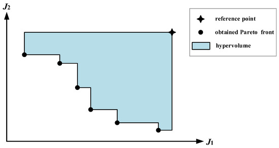
Figure 1.
Illustration of hypervolume with two objectives.
3. Experimental Results and Discussion
The proposed algorithms and methods were implemented in Python with the SPICE simulations conducted by the Cadence tool. Our experiments were run on an Intel Xeon Silver 2.4-GHz Linux workstation that has 512 G of memory. All the experiments were conducted in a CMOS 65-nm technology process.
3.1. Case Study 1: Two-Stage Op-Amp
The two-stage operational amplifier (Op-Amp) mainly consists of an active-loaded differential pair and a common-source amplifier, as shown in Figure 2. After considering the constraints of structure symmetry, 14 design variables (i.e., 5 transistor lengths, 5 transistor widths, 2 bias voltages, 1 resistance, and 1 capacitance) are identified to be optimized, which are labeled blue in Figure 2.
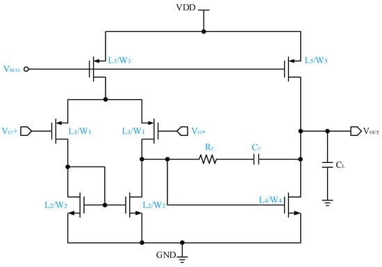
Figure 2.
Schematic of the two-stage Op-Amp.
To demonstrate the efficacy of our proposed group-based deterministic optimization algorithm (called Group-Deter) on this case-study circuit, we compared it with the deterministic optimization algorithm proposed in [16] (called Ori-Deter), our improved deterministic optimization algorithm in terms of new methods to calculate parameter correction and update design parameter values (called Impr-Deter), the PSO algorithm [3], the differential evolution (DE) algorithm [19], and the Bayesian optimization (BO) algorithm [7]. For the DE algorithm, the rand-to-best mutation strategy was employed.
In our experiments, we firstly randomly generated 20 sets of initial design points. For Group-Deter, PSO, and DE, they started optimization with these initial design points. For the Ori-Deter and Impr-Deter, we ran algorithms 20 times and each time started with one set of these initial design points to report the average results. The target performance specification was set as below:
where Av, UBW, and PM denote the DC gain, unity-gain bandwidth, and phase margin, respectively. Table 1 shows our experimental results. As one can see, although Impr-Deter used fewer iterations to achieve better maximal Av and mean Av than Ori-Deter, its performance still has some gap compared to Group-Deter, which achieved comparable performance with the well-known heuristic algorithms PSO, DE and BO but used fewer optimization iterations. These results demonstrate the advancement of our proposed Group-Deter.

Table 1.
Comparison among Six Single-Objective Optimization Algorithms for the Two-Stage Op-Amp.
To prove the effectiveness of our deterministic multi-objective optimization algorithm, we compared it with the NSGA-II, which is a well-known multi-objective optimization algorithm. We set the target performance specification to maximize the DC gain (i.e., Gain) and 3-dB bandwidth (i.e., BW) simultaneously while minimizing the quiescent power consumption (i.e., Power), which can be defined as follows:
The obtained Pareto front is shown in Figure 3, and the corresponding metrics calculation results are depicted in Table 2. From Table 2, it is evident that the Pareto front generated by our proposed method achieves a larger hypervolume and a smaller spacing metric compared to NSGA-II. These metrics, respectively, indicate that the Pareto front obtained by our method is closer to the ideal Pareto front with higher quality, and that the points on the Pareto front are more evenly distributed for the case-study circuit. Meanwhile, our proposed method uses a fewer number of simulations, indicating that it has a more efficient running speed. By systematically generating the weight vector and constructing the objective function, the obtained Pareto front distribution becomes more uniform.
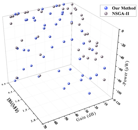
Figure 3.
Pareto fronts generated by our method and the NSGA-II for the two-stage Op-Amp.
Table 2.
Pareto Front Comparison of the Two-Stage Op-Amp.
3.2. Case Study 2: Folded-Cascode Op-Amp
The folded-Cascode Op-Amp is another case-study circuit, which is shown in Figure 4. It consists of a differential common-source amplifier and a differential common-gate amplifier loaded with a Cascode current source. Compared to the two-stage Op-Amp, the circuit structure of the folded-Cascode Op-Amp is more complex, which contains 17 design variables (i.e., 6 transistor lengths, 6 transistor widths, 5 bias voltages labeled blue in Figure 4) after considering the constraints of structure symmetry.
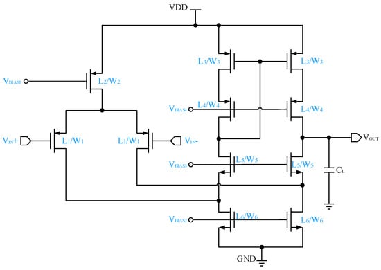
Figure 4.
Schematic of the folded-Cascode Op-Amp.
To test the effectiveness of our group-based deterministic optimization algorithm conducted on this case-study circuit, we used the same experimental settings as that of the case study of two-stage Op-Amp. Table 3 depicts the experimental results. As one can see, the Group-Deter used 17 iterations to reach the maximal Av of 68.13 dB, which indicates that it used fewer iterations than PSO, DE and BO but achieved comparable performance with them. Compared to Ori-Deter and Impr-Deter, the maximum Av reached by Group-Deter was much larger.
Table 3.
Comparison among Six Single-Objective Optimization Algorithms for the Folded-Cascode Op-Amp.
For analyzing our deterministic multi-objective optimization algorithm on this case-study circuit, the target performance specification was set to maximize DC gain while minimizing the power consumption, which can be represented as follows:
Figure 5 and Table 4 display the experimental results of the case-study circuit. As can be seen, compared with NSGA-II, the Pareto front obtained by our method is smoother and more evenly distributed, indicated by a larger hypervolume and a smaller spacing metric, respectively, while the number of simulations used by our method is fewer. This experiment demonstrates that our method can also effectively achieve multi-objective optimization in a more complex circuit.
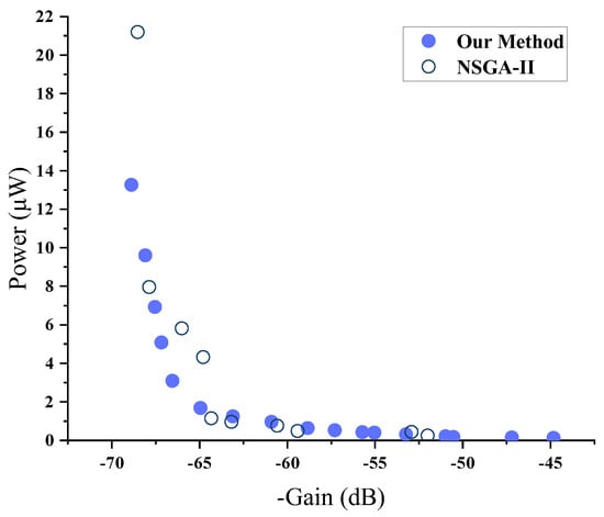
Figure 5.
Pareto front generated by our method and NSGA-II for the folded-Cascode Op-Amp.
Table 4.
Pareto Front Comparison of the Folded-Cascode Op-Amp.
3.3. Case Study 3: Three-Stage Op-Amp
The three-stage Op-Amp mainly consists of an active-loaded differential pair and a two-stage common-source amplifier, as shown in Figure 6. Compared to the two-stage Op-Amp, the three-stage Op-Amp has a higher gain but also consumes more power. After considering the constraints of structure symmetry, 19 design variables (i.e., 8 transistor lengths, 8 transistor widths, and 3 bias voltages) are identified to be optimized.
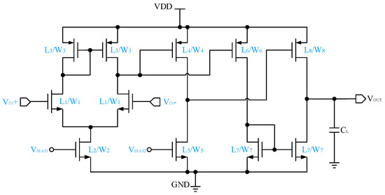
Figure 6.
Schematic of the three-stage Op-Amp.
For testing the advancement of our group-based deterministic optimization algorithm conducted on this case-study circuit, we used the same experimental settings as that of the case studies of two-stage Op-Amp and folded-Cascode Op-Amp. Table 5 depicts the experimental results. As one can see, the Group-Deter used 21 iterations to achieve the maximal Av of 97.4 dB, which is the best performance among all five algorithms. Moreover, compared with PSO, DE and BO, our Group-Deter also consumes fewer iterations than them.
Table 5.
Comparison among Six Single-Objective Optimization Algorithms for the Three-Stage Op-Amp.
For analyzing our deterministic multi-objective optimization algorithm on this case-study circuit, we set the performance specification to maximize DC gain while minimizing power consumption, which is defined as follows:
The Pareto front and the corresponding metrics values obtained from the experiment are shown in Figure 7 and Table 6, respectively. Although the number of design variables is increased compared to the former two case studies, our method still performs better than NSGA-II, which is reflected by better optimization results and higher optimization efficiency. Better optimization results of our method are indicated by a larger hypervolume and a smaller spacing metric while higher optimization efficiency is revealed by a fewer number of simulations used. This robustness demonstrates the capability of our method to effectively conduct multi-objective optimization of circuit performance, even for high-dimensional parameter spaces.
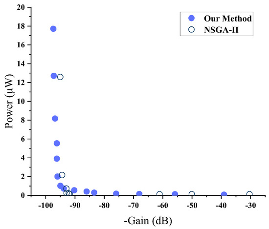
Figure 7.
Pareto front generated by our method and NSGA-II for the three-stage Op-Amp.
Table 6.
Pareto Front Comparison of the Three-Stage Op-Amp.
4. Conclusions
In this paper, we proposed a novel deterministic multi-objective optimization method. To realize deterministic multi-objective optimization, we firstly improved the efficiency and effectiveness of the single-objective deterministic optimization, making it able to efficiently and robustly figure out the global optimum. Then, the weighted sum method was employed to carry out multi-objective optimization by using our improved single-objective deterministic optimization method to derive the extremum of each circuit performance attribute. As experimental results demonstrated, our proposed deterministic multi-objective optimization method can produce better quality of Pareto front compared to the well-known NSGA-II algorithm.
Author Contributions
Conceptualization, Z.Z.; methodology, Z.X.; software, Z.X.; validation, J.L.; formal analysis, Z.Z.; investigation, Z.X.; resources, Z.Z.; data curation, Z.X.; writing—original draft preparation, Z.X.; writing—review and editing, Z.Z.; visualization, Z.X.; supervision, Z.Z. and J.L.; project administration, J.L.; funding acquisition, Z.Z. All authors have read and agreed to the published version of the manuscript.
Funding
This research was funded in part by the Postdoctoral Research Project Preferential Funding of Zhejiang Province, China under grant number ZJ2023003 and in part by the National Natural Science Foundation of China under grant number 62331018. The APC was funded by ZJ2023003.
Data Availability Statement
Dataset available on request from the authors.
Conflicts of Interest
The authors declare no conflicts of interest.
References
- Fayazi, M.; Colter, Z.; Afshari, E.; Dreslinski, R. Applications of Artificial Intelligence on the Modeling and Optimization for Analog and Mixed-Signal Circuits: A Review. IEEE Trans. Circuits Syst. I Regul. Pap. 2021, 68, 2418–2431. [Google Scholar] [CrossRef]
- Thongkrairat, S.; Chutchavong, V. Hard Deterministic Particle Swarm Optimisation for Certain Result Solution. In Proceedings of the 2021 International Conference on Electronics, Information, and Communication (ICEIC), Jeju, Republic of Korea, 31 January–3 February 2021; pp. 1–4. [Google Scholar]
- Vural, R.A.; Yildirim, T. Analog circuit sizing via swarm intelligence. AEU—Int. J. Electron. Commun. 2012, 66, 732–740. [Google Scholar] [CrossRef]
- Martins, R.; Lourenço, N.; Póvoa, R.; Horta, N. Shortening the gap between pre- and post-layout analog IC performance by reducing the LDE-induced variations with multi-objective simulated quantum annealing. Eng. Appl. Artif. Intell. 2021, 98, 104102. [Google Scholar] [CrossRef]
- Saǧlican, E.; Afacan, E. MOEA/D vs. NSGA-II: A Comprehensive Comparison for Multi/Many Objective Analog/RF Circuit Optimization through a Generic Benchmark. ACM Trans. Des. Autom. Electron. Syst. 2023, 29, 1–23. [Google Scholar] [CrossRef]
- Pramanik, A.K.; Bhowmik, D.; Pal, J.; Sen, P.; Saha, A.K.; Sen, B. Towards the realization of regular clocking-based QCA circuits using genetic algorithm. Comput. Electr. Eng. 2022, 97, 107640. [Google Scholar] [CrossRef]
- Lyu, W.; Xue, P.; Yang, F.; Yan, C.; Hong, Z.; Zeng, X.; Zhou, D. An Efficient Bayesian Optimization Approach for Automated Optimization of Analog Circuits. IEEE Trans. Circuits Syst. I Regul. Pap. 2018, 65, 1954–1967. [Google Scholar] [CrossRef]
- Długosz, Z.; Rajewski, M.; Długosz, R.; Talaśka, T.; Pedrycz, W. A new deterministic PSO algorithm for real-time systems implemented on low-power devices. J. Comput. Appl. Math. 2023, 429, 115225. [Google Scholar] [CrossRef]
- Martins, R.; Lourenço, N.; Horta, N. Multi-objective optimization of analog integrated circuit placement hierarchy in absolute coordinates. Expert Syst. Appl. 2015, 42, 9137–9151. [Google Scholar] [CrossRef]
- Liao, T.; Zhang, L. Efficient parasitic-aware hybrid sizing methodology for analog and RF integrated circuits. Integration 2018, 62, 301–313. [Google Scholar] [CrossRef]
- Zadeh, L. Optimality and non-scalar-valued performance criteria. IEEE Trans. Autom. Control 1963, 8, 59–60. [Google Scholar] [CrossRef]
- De Smedt, B.; Gielen, G. WATSON: A multi-objective design space exploration tool for analog and RF IC design. In Proceedings of the IEEE 2002 Custom Integrated Circuits Conference (Cat. No.02CH37285), Orlando, FL, USA, 15 May 2002; pp. 31–34. [Google Scholar]
- Rout, P.K.; Acharya, D.P. Fast physical design of CMOS ROs for optimal performance using constrained NSGA-II. AEU—Int. J. Electron. Commun. 2015, 69, 1233–1242. [Google Scholar] [CrossRef]
- Deb, K.; Pratap, A.; Agarwal, S.; Meyarivan, T. A fast and elitist multiobjective genetic algorithm: NSGA-II. IEEE Trans. Evol. Comput. 2002, 6, 182–197. [Google Scholar] [CrossRef]
- Yin, S.; Wang, R.; Zhang, J.; Liu, X.; Wang, Y. Fast Surrogate-Assisted Constrained Multiobjective Optimization for Analog Circuit Sizing via Self-Adaptive Incremental Learning. IEEE Trans. Comput.-Aided Des. Integr. Circuits Syst. 2023, 42, 2080–2093. [Google Scholar] [CrossRef]
- Schwencker, R.; Eckmueller, J.; Graeb, H.; Antreich, K. Automating the sizing of analog CMOS circuits by consideration of structural constraints. In Proceedings of the Design, Automation and Test in Europe Conference and Exhibition, Munich, Germany, 9–12 March 1999; pp. 323–327. [Google Scholar]
- Dong, X.; Zhang, L. PV-Aware Analog Sizing for Robust Analog Layout Retargeting with Optical Proximity Correction. ACM Trans. Des. Autom. Electron. Syst. 2018, 23, 1–19. [Google Scholar] [CrossRef]
- Ahmadi, B.; Ceylan, O.; Ozdemir, A. Reinforcement of the distribution grids to improve the hosting capacity of distributed generation: Multi-objective framework. Electr. Power Syst. Res. 2023, 217, 109120. [Google Scholar] [CrossRef]
- Yin, S.; Zhang, W.; Hu, W.; Wang, Z.; Wang, R.; Zhang, J.; Wang, Y. An efficient reference-point based surrogate-assisted multi- objective differential evolution for analog/RF circuit synthesis. In Proceedings of the IEEE International Symposium on Radio-Frequency 391 Integration Technology (RFIT), Hualien, Taiwan, 25–27 August 2021. [Google Scholar]
Disclaimer/Publisher’s Note: The statements, opinions and data contained in all publications are solely those of the individual author(s) and contributor(s) and not of MDPI and/or the editor(s). MDPI and/or the editor(s) disclaim responsibility for any injury to people or property resulting from any ideas, methods, instructions or products referred to in the content. |
© 2024 by the authors. Licensee MDPI, Basel, Switzerland. This article is an open access article distributed under the terms and conditions of the Creative Commons Attribution (CC BY) license (https://creativecommons.org/licenses/by/4.0/).