Improved Convolutional Neural Network for Wideband Space-Time Beamforming

Abstract

Wideband beamforming technology is an effective solution in millimeter-wave (mmWave) massive multiple-input multiple-output (MIMO) systems to compensate for severe path loss through beamforming gain. However, traditional adaptive wideband digital beamforming (AWDBF) algorithms suffer from serious performance degradation when there are insufficient signal snapshots, and the training process of the existing neural network-based wideband beamforming network is slow and unstable. To address the above issues, an AWDBF method based on the convolutional neural network (CNN) structure, the improved wideband beamforming prediction network (IWBPNet), is proposed. The proposed method increases the network’s feature extraction capability for array signals through deep convolutional layers, thus alleviating the problem of insufficient network feature extraction capabilities. In addition, the pooling layers are introduced into the IWBPNet to solve the problem that the fully connected layer of the existing neural network-based wideband beamforming algorithm is too large, resulting in slow network training, and the pooling operation increases the generalization ability of the network. Furthermore, the IWBPNet has good wideband beamforming performance with low signal snapshots, including beam pattern performance and output signal-to-interference-plus-noise ratio (SINR) performance. The simulation results show that the proposed algorithm has superior performance compared with the traditional wideband beamformer with low signal snapshots. Compared with the wideband beamforming algorithm based on the neural network, the training time of IWBPNet is only $10.6\%$ of the original neural network-based wideband beamformer, while the beamforming performance is slightly improved. Simulations and numerical analyses demonstrate the effectiveness and superiority of the proposed wideband beamformer.

1. Introduction

Beamforming is a spatial filtering technique used to enhance signals in a specific direction while suppressing signals from other directions [1,2,3]. Based on the bandwidth of the processed signal, they can be categorized into two groups, namely narrowband beamforming and wideband beamforming [4,5,6]. Traditional beamforming studies mainly focus on the narrowband field. As the signal propagation environment becomes more and more complex, adaptive wideband digital beamforming (AWDBF) has been broadly utilized in many fields such as radio communications, radar, sonar, microphone arrays, seismology, astronomy and medical imaging [7,8,9].

Based on the processing domain of the received signal, the adaptive wideband beamforming algorithms can be categorized into spatial-temporal and spatial-frequency beamforming, respectively [10,11,12]. Frost beamformer (FB) is a well-known wideband space-time beamformer that employs a series of tapped delay lines (TDLs) for frequency-dependent weighting [13]. The FB utilizes the linearly constrained minimum variance (LCMV) criterion and can effectively achieve real-time wideband beamforming. To achieve accurate beam pointing and undistorted response to the signals of interest (SOIs), the pre-steering delay structures are utilized to correct the misalignment between SOI orientation and array geometry. However, this structure often has time-delay errors in practical applications, resulting in serious deterioration in performance [6,14]. Therefore, convolution constraints are introduced to remove the pre-steering delay structures [15], while this algorithm adds additional computational complexity. Then, the frequency constraint matrix is introduced to eliminate the pre-steering delay structures, namely frequency-constrained FB (FCFB) [16]. This method eliminates the pre-steering delay structures without increasing computational complexity and demonstrates good performance. Nonetheless, the FCFB still requires multiple adaptive weights to achieve a satisfactory output signal-to-interference-plus-noise ratio (SINR), resulting in poor performance in real-time calculations. Moreover, the traditional AWDBF algorithm cannot effectively generate a gain for the SOI and suppress the jamming sources when there are insufficient signal snapshots, leading to significant performance degradation.

Deep learning (DL) has experienced rapid development in recent years, finding widespread applications across various domains, such as target recognition and image classification [17,18,19]. Among the crucial models within DL, the convolutional neural network (CNN) stands out. It boasts essential features such as local connections, weight sharing, and multi-level feature learning. This network model significantly reduces the number of parameters, rendering it a potent instrument for tackling numerous intricate problems. CNNs have been utilized in the field of beamforming to obtain better beamforming performance. In [20], a radial basis function (RBF) based method using a two-stage CNN is proposed, which can perform beamforming without requiring model parameters, and has good accuracy and robust performance. A novel robust adaptive beamforming approach is proposed [21], where the signal covariance matrix is utilized as training data, and it achieves the purpose of calculating the beamforming weights directly from the signal covariance matrix. However, the process of solving the signal covariance matrix still has some complexity when compared with directly obtaining information from the received array signal. In [22], the CNN is utilized to the transmitter and trained in a supervised manner considering both uplink and downlink transmissions. However, the above-mentioned methods of applying neural networks to the field of beamforming to improve the performance of traditional beamformers focus on the narrowband beamforming. The model establishment in the field of wideband beamforming is more complex, and the number of parameters is larger. Applying deep learning to wideband beamforming to reduce complexity is meaningful. A frequency constraint wideband beamforming prediction network (WBPNet) based on the CNN is proposed in [23], which maintains good beam pointing under low-signal snapshots. However, the proposed method just preliminarily explores the possibility of a wideband beamforming algorithm based on deep learning. The network structure utilized is just a simple stack of three convolutional layers, and the large fully connected layer leads to the network difficult to train. A neural network-based wideband beamformer using progressive learning to train the network is proposed [24]. Although the training time is reduced, it still takes about one hour.

Pooling layers (PLs) [25,26,27,28] can significantly reduce the spatial dimension of the input and prevent overfitting of the network, thus reducing computational costs and improving network performance [29]. Moreover, the pooling technology can significantly and effectively reduce model training time, making beamforming more economical [26].

Based on the WBPNet, a new network structure for wideband beamforming weights generation is explored, named improved WBPNet (IWBPNet). The strong points of the proposed method are as follows. Firstly, to solve the problem of insufficient feature extraction capability of WBPNet, the network layer is added to improve the network’s ability to extract the features of array signals. Moreover, to solve the problem that the parameters of WBPNet are too large, resulting in the network training time is long, and the generalization ability is insufficient, PL is introduced into the IWBPNet to reduce the number of parameters that need to be trained, which makes the network easier to train and improves the generalization ability of the network. Through the above methods, the proposed IWBPNet shows superior performance compared with the WBPNet. In terms of network training speed, the training time of IWBPNet is $0.3683$ h, which is only $10.6\%$ of WBPNet training time. In terms of beamforming performance, while maintaining good beam pattern performance, the output SINRs of IWBPNet have a small improvement. Compared with the method in [24], the proposed IWBPNet saves $64.1\%$ of training time while ensuring beamforming performance.

The rest of the paper is organized as follows: Section 2 introduces the conventional wideband beamforming method, FB and FCFB. In Section 3, a more economical network structure for the adaptive spatial-temporal wideband beamforming is presented, which greatly improves the problem of long network training time. In Section 4, the simulation results and analyses are given to show the correctness and effectiveness of the proposed algorithm. Finally, the brief conclusions can be found in Section 5.

2. Traditional Space-Time Wideband Beamformers

In wideband beamformers, new dimensions are usually added on the basis of the spatial dimension to achieve the frequency-dependent response to wideband signals. Among them, the famous FB achieves the above response by adding TDLs after the array element, thereby increasing the time dimension. In this section, we provide a brief overview of traditional wideband beamformers, including key structures and implementation methods of the FB and the FCFB.

2.1. Wideband FB with Pre-Steering Delay Structures

Assume that there is a one-dimensional uniform linear array (ULA) consisting of a total of J array elements, with each array element being equipped with K delay structures. The spacing between adjacent array elements is set as d, which corresponds to half of the wavelength, denoted as $\lambda$, at the highest frequency to avoid the occurrence of grating lobes. The incoming signal approaches the array from the far field with lightspeed, denoted as c, and can be treated as a parallel plane wave.

FB can adjust the sensor array in real time to respond to the SOI and suppress noise signals. The basic idea is to dynamically adjust the weights of a wideband sensor array, thereby minimizing the noise power of the array output and maintaining a satisfactory response to the direction of SOI [13]. In order to ensure that the signal from the desired direction has coherence when output, the pre-steering delay structures are utilized in the FB. The wideband FB with pre-steering delays is shown in Figure 1. Thereinto, $T_j\left({\theta }_0\right)=\left(j-1\right)\frac{dsin{\theta }_0}{c},\left(j=1,2,\dots ,J\right)$ are the pre-steering delays, and $R_k\left(z\right)$ is given as

$$\left\{\begin{array}{c}{R}_1\left(z\right)=1\hfill \\ R_k\left(z\right)=z^{-1}k=2,3,\dots ,K.\hfill \end{array}\right.$$

(1)

Then, the signal of each tap can be written as

$$x_{j,k}\left(n\right)=x_j[n-(k-1)\tau ]$$

(2)

where $j=1,2,\dots ,J$, $k=1,2,\dots ,K$, and $\tau$ denotes the time delay between adjacent taps.

At the n-th, the $JK\times 1$ signal vector $\mathbf{x}\left(n\right)$ can be expressed as

$$\begin{array}{c}\mathbf{x}\left(n\right)=\left[x_{1,1}\left(n\right),\dots ,x_{J,1}\left(n\right),x_{1,2}\left(n\right),\right.{\left.\dots ,x_{1,K}\left(n\right),\dots ,x_{J,K}\left(n\right)\right]}^T.\hfill \end{array}$$

(3)

The $JK\times 1$ adaptive weight vector $\mathbf{w}$ is

$$\mathbf{w}={\left[w_{1,1},\dots ,w_{J,1},w_{1,2},\dots ,w_{1,K},\dots ,w_{J,K}\right]}^T.$$

(4)

Finally, the output of the beamformer can be represented as

$$y\left(n\right)={\mathbf{w}}^H\mathbf{x}\left(n\right),$$

(5)

where ${[•]}^H$ represents the conjugate transpose.

2.2. Wideband FB Based on Frequency Constraints

The pre-steering delay structures in Section 2.1 may produce time-delay errors and the FB needs K degrees of freedom (DOFs) to satisfy the constraints, weakening anti-interference ability [6]. To effectively address this problem, one viable solution is to introduce an additional set of frequency domain constraints, i.e., the FCFB.

Different from the beamformer presented in Figure 1, consider a signal with bandwidth f, the minimum frequency of which is $f_{min}$, and the maximum frequency is $f_{max}$, i.e., $f_i\in [f_{min},f_{max}]$, $i=1,2,\dots ,I$. Then, the wideband signal is evenly divided into I sub-bands, the frequency domain constraint matrix is expressed as

$${\mathbf{C}}_F={\left[{\mathbf{c}}_F\left(f_1\right),{\mathbf{c}}_F\left(f_2\right),\dots ,{\mathbf{c}}_F\left(f_i\right),\dots ,{\mathbf{c}}_F\left(f_I\right)\right]}_{JK\times I}$$

(6)

where ${\mathbf{c}}_F\left(f_i\right)$ is a $JK\times 1$ column vector expressed as

$${\mathbf{c}}_F\left(f_i\right)={\mathbf{c}}_{F,T_s}\left(f_i\right)\otimes {\mathbf{c}}_{F,T}\left(f_i\right),$$

(7)

where ⊗ is the Kronecker product,

$${\mathbf{c}}_{F,T_s}\left(f_i\right)={\left[1,e^{-j2\pi f_i{T}_s},\dots ,e^{-j2\pi f_i(K-1)T_s}\right]}^T,$$

(8)

and

$$\begin{array}{c}{\mathbf{c}}_{F,T}\left(f_i\right)=\left[e^{-j2\pi f_i{T}_1\left({\theta }_0\right)},e^{-j2\pi f_i{T}_2\left({\theta }_0\right)},\right.{\left.\dots ,e^{-j2\pi f_i{T}_J\left({\theta }_0\right)}\right]}^T.\hfill \end{array}$$

(9)

The response vector corresponding to ${\mathbf{C}}_F$ is ${\mathbf{f}}_F$, which can be expressed as

$$\begin{array}{c}{\mathbf{f}}_F=\left[e^{-j2\pi f_1(K-1)/2},e^{-j2\pi f_2(K-1)/2},\right.{\left.\dots ,e^{-j2\pi f_I(K-1)/2}\right]}^T.\hfill \end{array}$$

(10)

According to Equation (3), the correlation matrix of the signal can be denoted as

$${\mathbf{R}}_{xx}=E\left\{\mathbf{x}\left(n\right){\mathbf{x}}^H\left(n\right)\right\},$$

(11)

thereinto, $E\{•\}$ is the expectation operation.

Consider a radar system with the intermittent period. During the radar intermittent period, the signal received by the array only contains noise and interference, so ${\mathbf{R}}_{xx}$ is the covariance matrix of noise plus interference. Under the LCMV criterion, the AWDBF problem can be formulated as the following optimization formula

$$\left\{\begin{array}{cc}\underset{\mathbf{w}}{min}\hfill & {\mathbf{w}}^H{\mathbf{R}}_{i+n}\mathbf{w}\hfill \\ s.t.\hfill & {{\mathbf{C}}_F}^H\mathbf{w}={\mathbf{f}}_F,\hfill \end{array}\right.$$

(12)

where ${\mathbf{R}}_{i+n}$ represents the covariance matrix of interference signals plus noise. According to the Lagrange criterion, the optimization problem in Equation (12) can be transformed into an elegant expression [16]

$${\mathbf{w}}_{opt}={\mathbf{R}}_{i+n}^{-1}{\mathbf{C}}_F{\left[{{\mathbf{C}}_F}^H{\mathbf{R}}_{i+n}^{-1}{\mathbf{C}}_F\right]}^{-1}{\mathbf{f}}_F.$$

(13)

Then, the output of the FCFB can be obtained from Equation (5).

Output SINR is an important indicator for evaluating beamforming performance, which reflects the effect of the beamformer on enhancing desired signal and suppressing interference signals and noise. It can be calculated by

$$\mathrm{SINR}=\frac{{{\mathbf{w}}_{opt}}^H{\mathbf{R}}_s{\mathbf{w}}_{opt}}{{{\mathbf{w}}_{opt}}^H{\mathbf{R}}_{i+n}{\mathbf{w}}_{opt}},$$

(14)

where ${\mathbf{R}}_s$ is the covariance matrix of the desired signal.

3. The Improved Adaptive Wideband Beamforming Method Based on Machine Learning

The beamforming weights of traditional algorithms require the covariance matrix of interference plus noise. In actual situations, the covariance matrix can only be estimated based on a finite number of signal snapshots, and the accuracy of the estimated covariance matrix is closely related to the number of snapshots. When the number of snapshots is insufficient, the performance of traditional wideband beamforming will deteriorate severely. To solve this problem, the neural network-based wideband beamformer has emerged. However, the wideband beamforming algorithm cannot be regarded as a simple superposition of the narrowband beamforming algorithm. It usually introduces a new dimension for frequency correlation of the wideband signal, which is a complex process. The wideband beamforming algorithm based on neural networks is in the early stages of research, and has problems such as unstable network training and long network training time. In this section, an improved neural network-based wideband beamforming algorithm is introduced to solve the problem of long training time.

3.1. The Structure of the Improved Neural Network

CNNs possess unique attributes that enhance their efficiency and effectiveness in various tasks. One of the key strengths is local awareness, which allows them to concentrate on specific local regions within the input, thus reducing computational complexity. Furthermore, CNNs utilize parameter sharing, which allows the same set of weights to process different regions of the input. This feature reduces the number of parameters in the network and mitigates overfitting.

Neural networks constructed with multiple convolutional layers exhibit a hierarchical learning capability. Each layer is capable of learning features at different levels of abstraction. This hierarchical learning empowers the network to automatically extract features ranging from low-level details to high-level patterns, thereby enhancing its overall performance.

In this section, an improved neural network-based wideband beamforming method is proposed to solve the problems of long training time in existing neural network-based methods caused by too many network parameters. The improved neural network structure is depicted in Figure 2.

The input feature map has a size of 16 by 400 with 2 channels. Thereinto, the values 16 and 400 correspond to the width and height of the feature map, while 2 signifies the number of channels. In array signal processing, the received data and weights for beamforming are usually in complex form. Therefore, dual channels are used for data transmission, where one channel transmits the real part and the other transmits the imaginary part of the complex-valued data.

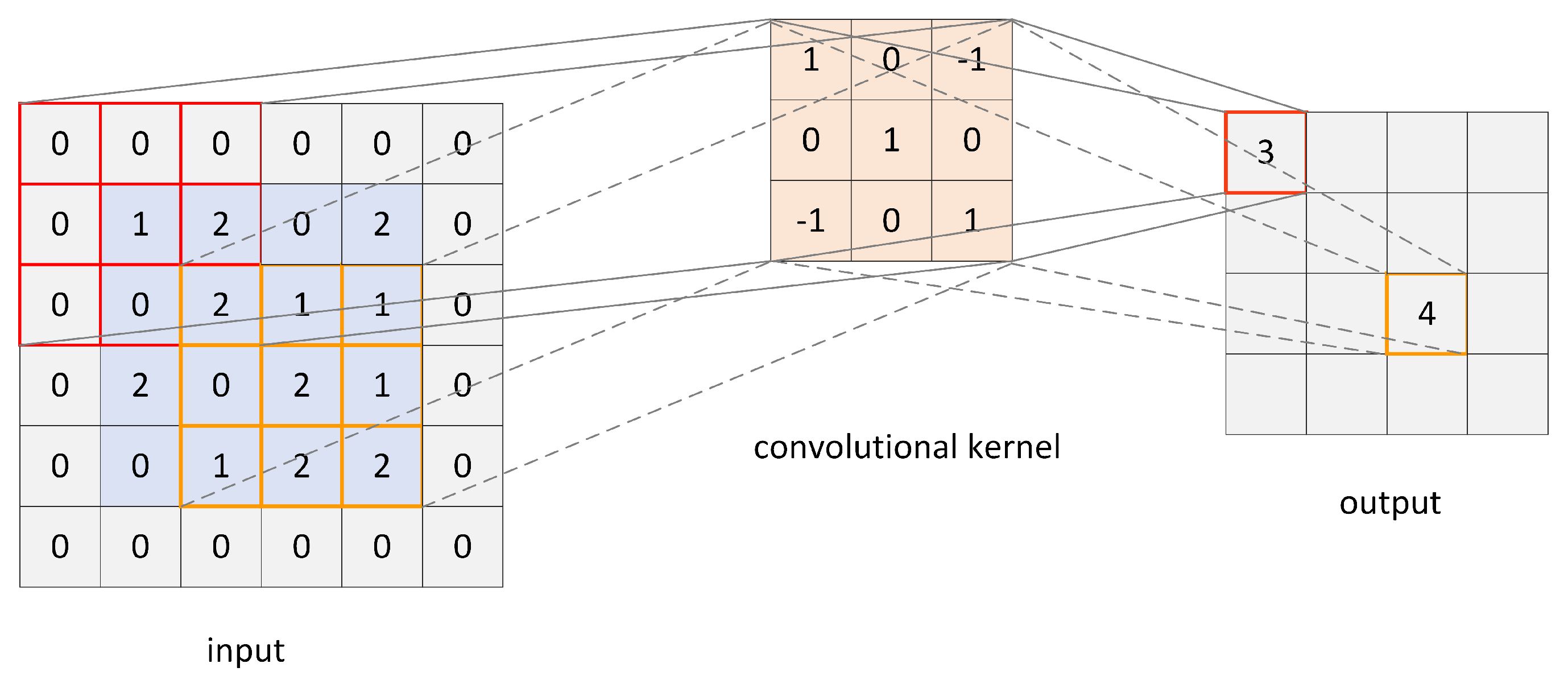
Then, the data enters the convolutional layer, which processes the information of each small area, reducing the amount of parameters while maintaining the continuity of the information. The process can be expressed as

$$Output=\sum _i{w}_i{x}_i+b,$$

(15)

where $x_i$ and $w_i$ denote the input data and the weight of the convolutional kernel, respectively. b is the bias term.

Figure 3 illustrates a simple schematic diagram of the convolutional process. All of the information in the diagram is hypothetical and intended to illustrate the convolution process, and the bias is set as zero.

As can be seen from the diagram, when the input is convolved according to Equation (15), the convolution kernel remains consistent. This feature reduces the number of parameters that need to be updated during network training process. In this paper, the size of the convolution kernel is set as $3\times 3$, and the padding and stride are both set as 1.

Then, the batch normalization [30] layers are utilized, which can accelerate the convergence speed during model training, enhance the stability of the training process, prevent issues such as gradient explosions or vanishing, and introduce a beneficial regularization effect. Subsequently, max pooling operations are used in the first three layers of the network to reduce feature dimensions, model complexity, and mitigate the risk of overfitting. The schematic diagram of the max pooling operation is shown in Figure 4.

The Leaky Rectified Linear Unit (LeakyReLU) [31] is utilized as the activation function, and can be expressed as

$$\mathrm{LeakyReLU}\left(x\right)=\left\{\begin{array}{cc}x,\hfill & x\ge 0\hfill \\ \alpha x,\hfill & x<0.\hfill \end{array}\right.$$

(16)

where $\alpha$ is a coefficient, typically assigned a value of $0.01$.

Finally, the data are flattened and then passes through the FC layer to achieve classification output of the data.

3.2. Training Process of the Improved Network

First, in the case of low snapshots, 500 sets of training data and 10 sets of test data are generated for neural network training. The data set consists of array received signals directly. Then, under the high snapshot scenarios, according to Equation (13), the analytical solution of optimal weights for the traditional wideband beamforming method, FCFB, is utilized to generate the weights ${\mathbf{w}}_{opt}$ required for wideband beamforming. The weights also serve as the target labels that the neural network aims to fit during the training process.

Moreover, the Adam algorithm [32] is utilized to adaptively adjust the learning rate. This aids in achieving faster convergence during the early stages of training and ensures that the learning rate decreases as the optimal solution is approached, thus preventing the possibility of skipping the optimal solution. The initial learning rate used in training is $0.0006$, the adaptive attenuation factor is $0.7$, and the attenuation step is 20. The batch size is set as 16. The signal with low snapshots and the beamforming weights obtained with high snapshots are used as the input and label of the network, respectively, to achieve the mapping between the low-snapshot signal and the wideband beamforming weights. The loss function during network training is expressed as follows:

$$Loss=\sum _{m=1}^M\frac{{\left|y_{trai{n}_m}-y_m\right|}^2}{M},$$

(17)

where M is the number of outputs. $y_{train}$ and y denote the label and output of the network, the goal of training is to minimize the loss function $L(y_{train},y)$.

After successful training, the network can map input signals to corresponding wideband beamforming weights at low snapshots. This means that we only need to feed low-snapshot signals into the network to quickly obtain the corresponding weights, significantly reducing the waiting time during system sampling.

4. Simulation Results

In this section, we compare the IWBPNet with the WBPNet and traditional FCFB in terms of beam pattern performance and output SINRs. Moreover, the proposed method is compared with the method in [24], the broadband beamforming weight generation network (BWGN). All simulations in this article are conducted under the PyTorch framework, the version is $\mathrm{2.0.0}$, and the Python version is $3.8$. A total of 40 Monte Carlo simulations are carried out for all results.

The simulation is carried out under the following conditions. The number of ULA antennas J and delay structures after each antenna element K are 16 and 18, respectively. The number of sub-bands I, is set as 10. Assume that a wideband desired signal comes from ${\theta }_0=5^{\circ }$, and the interference plus noise signals ${\theta }_j$ come from the range $[-{60}^{\circ },-{30}^{\circ }]$, i.e., ${\theta }_j\in [-{60}^{\circ },-{30}^{\circ }]$.

For simplicity and clarity of description, we define some abbreviations. The traditional beamforming method, FCFB, under sufficient signal snapshots, is defined as FCFB-SS. While that under insufficient signal snapshots is defined as FCFB-IS. The WBPNet under insufficient signal snapshots, is defined as WBPNet-IS. Similarly, the improved CNN structure for AWDBF under insufficient snapshot scenarios is defined as IWBPNet-IS, and the BWGN with insufficient snapshots is defined as BWGN-IS. The number of sufficient snapshots and insufficient snapshots are set as 4000 and 400, respectively. In addition, $f_{min}$ and $f_{max}$ are set as $0.8$ GHz and $1.1$ GHz, respectively. Gaussian white noise with a mean of 0 and a variance of 1 is added to simulate the environment. The interference-to-noise ratio (INR) and signal-to-noise ratio (SNR) are assumed as 40 dB and 0 dB.

Without loss of generality, the following three interference angles are randomly selected to evaluate the performance of the beam pattern, that is: ${\theta }_{j1}$, ${\theta }_{j2}$, ${\theta }_{j3}$, at $-{60}^{\circ }$, $-{40}^{\circ }$, $-{30}^{\circ }$, respectively. Figure 5 shows the beam patterns of FCFB-SS and FCFB-IS for the desired and interference signals from the following directions: (${\theta }_0,{\theta }_{j1}$), (${\theta }_0,{\theta }_{j2}$) and (${\theta }_0,{\theta }_{j3}$); and (${\theta }_0,{\theta }_{j1}$) represents the desired signal comes from ${\theta }_0$ and the interference signal comes from ${\theta }_{j1}$. The beam patterns of WBPNet-IS, BWGN-IS and IWBPNet-IS are illustrated in Figure 6.

The beam patterns presented in Figure 5 show that the traditional beamformer, FCFB, has good performance under high snapshots, but when the snapshots are insufficient, the performance deteriorates seriously. In contrast, from Figure 6, the WBPNet, BWGN and IWBPNet all have a high gain in the SOI direction and a deep null in the interference direction, although the number of signal snapshots is insufficient. This is due to the powerful nonlinear fitting ability of neural networks, which can fully learn the intrinsic relationship between the input data and output weights used for wideband beamforming with limited snapshots. After the network is successfully trained, we only need to provide the network with insufficient snapshot data, and the network can quickly generate good weights required for wideband beamforming, which significantly reduces the sampling time.

However, due to the large number of fully connected layers in WBPNet and the lack of necessary network optimization, which is just a stack of three convolutional networks, WBPNet takes a long time to train and is unstable. Due to the two-dimensional complex network structure in BWGN, the network training process is relatively complicated, which affects the network training speed. The WBPNet, BWGN and IWBPNet are all trained under the same parameters for 300 epochs. The training process of the WBPNet takes $3.4821$ h, the training process of the BWGN takes $1.0262$ h, while the IWBPNet just spends $0.3683$ h to train, saving $89.4\%$ of the time compared with WBPNet and $64.1\%$ compared with BWGN, which is a huge improvement. The results show that while maintaining good wideband beamforming performance, the training time of IWBPNet is significantly reduced compared to the other two networks. Considering the application of neural network-based wideband beamformers are needed online training in real-time systems, less network training time is of great significance while maintaining good performance. Reducing the network training time while maintaining good beamforming performance is also the core of this research.

Furthermore, the output SINRs of FCFB with 400 and 4000 signal snapshots, and output SINRs of WBPNet, BWGN and IWBPNet with 400 signal snapshots at different interference angles are shown in

Table 1. The output SINRs of FCFB with 400 and 4000 signal snapshots, and output SINRs of WBPNet, BWGN and IWBPNet with 400 signal snapshots at different interference angles.

Direction	FCFB-SS (N = 4000)	FCFB-IS (N = 400)	WBPNet-IS (N = 400)	BWGN-IS (N = 400)	IWBPNet-IS (Proposed) (N = 400)
(${\theta }_0,{\theta }_{j1}$)	4.4021	−14.4238	4.2688	4.2921	4.2998
(${\theta }_0,{\theta }_{j2}$)	4.3948	−13.8246	4.2156	4.3466	4.3720
(${\theta }_0,{\theta }_{j3}$)	4.3663	−14.2101	4.2697	4.2058	4.3178

. The results show that FCFB has good SINR performance when the signal snapshots are sufficient, because the covariance matrix of the array received signals is estimated approximately accurately. However, when the number of signal snapshots is insufficient, the estimated covariance matrix will be wrong, resulting in severe degradation of SINR performance. In contrast, the SINRs of WBPNet-IS, BWGN-IS and IWBPNet-IS demonstrate that the neural network-based wideband beamformers have good SINR performance despite the number of signal snapshots is insufficient. This is because the neural network has a strong fitting ability and can extract the characteristics of the array signals from a limited number of snapshots, resulting in good performance. Compared with the WBPNet, the IWBPNet demonstrates better SINR performance with insufficient snapshots. This is attributed to the IWBPNet having a deeper network structure, which increases the network’s ability to extract signal features. In addition, the PLs reduce the risk of network overfitting and greatly improve the generalization ability of the network. Compared with BWGN, the SINR performance of IWBPNet is also slightly improved due to the stronger generalization ability of IWBPNet. And the network training time of IWBPNet is only $35.9\%$ of training BWGN, demonstrating great time advantage of the proposed method. The simulation results of beam patterns, training time and SINRs for FCFB, WBPNet, BWGN and IWBPNet manifest the effectiveness and superiority of the proposed IWBPNet compared with the traditional wideband beamformer and the existing neural network-based wideband beamformers.

5. Conclusions

In this paper, for the neural network-based wideband beamformers, we start from the perspective that real-time training is required in actual systems due to environmental changes, and are committed to reducing the network training time while maintaining the performance of wideband beamforming. An improved neural network-based wideband beamformer, IWBPNet, is proposed to address the problem of long network training time of the existing neural network-based wideband beamforming algorithms. The improved structure utilizes the neural network to express the nonlinear mapping between the input signal and the weights used for AWDBF, which increases the number of network layers compared with WBPNet, thereby improving the network’s ability to extract signal features. In addition, the pooling layers are added to reduce the dimension of data transmission in the network, thus increasing the generalization ability of the network and solving the problem of too large fully connected layer in WBPNet. The proposed algorithm has great advantages in training time. Simulation results demonstrate that the training time of the proposed algorithm is $0.3683$ h, which saves $89.4\%$ of the time compared with WBPNet. Compared with BWGN, the proposed method saves $64.1\%$ of the time. Moreover, due to the better fitting and generalization capabilities of the improved network, the proposed algorithm has better SINR performance.