Contrastive Learning Joint Regularization for Pathological Image Classification with Noisy Labels

Abstract

The annotation of pathological images often introduces label noise, which can lead to overfitting and notably degrade performance. Recent studies have attempted to address this by filtering samples based on the memorization effects of DNNs. However, these methods often require prior knowledge of the noise rate or a small, clean validation subset, which is extremely difficult to obtain in real medical diagnosis processes. To reduce the effect of noisy labels, we propose a novel training strategy that enhances noise robustness without prior conditions. Specifically, our approach includes self-supervised regularization to encourage the model to focus more on the intrinsic connections between images rather than relying solely on labels. Additionally, we employ a historical prediction penalty module to ensure consistency between successive predictions, thereby slowing down the model’s shift from memorizing clean labels to memorizing noisy labels. Furthermore, we design an adaptive separation module to perform implicit sample selection and flip the labels of noisy samples identified by this module and mitigate the impact of noisy labels. Comprehensive evaluations of synthetic and real pathological datasets with varied noise levels confirm that our method outperforms state-of-the-art methods. Notably, our noise handling process does not require any prior conditions. Our method achieves highly competitive performance in low-noise scenarios which aligns with current pathological image noise situations, showcasing its potential for practical clinical applications.

1. Introduction

In recent years, deep neural networks (DNNs) have achieved significant developments in pathological image classification. Through multilayer nonlinear transformations and feature extraction, DNNs can learn higher-level feature representations from pathological images, thereby achieving accurate classification and diagnosis. However, noisy labels in pathological images pose some challenges when applying DNNs. The noisy label problem primarily arises from the annotation process of pathological images. The annotation of pathological images typically relies on the knowledge and experience of professional doctors. However, subjective judgments, human errors, and device noise may exist during the annotation process, leading to label uncertainty or errors. Additionally, the annotation cost for large-scale datasets is high, and oversights and mistakes during the annotation process are inevitable. These problems result in the presence of noisy labels in pathological images.

It is generally believed that DNNs possess exceptionally powerful mapping capabilities to the extent that they can easily memorize all sample data during the training process, including noisy labels. The memorization of noisy labels leads to a degradation in the model’s generalization ability, and as the noise rate increases, the generalization performance decreases accordingly. Therefore, noise-resistant training methods are urgently needed for pathological image classification tasks. Previous studies [1,2,3,4] have demonstrated that DNNs first memorize simple samples and then memorize the remaining samples. Based on this observation, some studies [5,6,7,8,9,10] have proposed methods that utilize the loss values of samples to judge their cleanliness. They believe that samples with smaller loss values are more likely to be clean samples, while samples with larger loss values are more likely to be noisy samples. By training on the selected small-loss samples, the generalization ability of the model can be improved. However, this judgment criterion could be clearer and more effectively distinguish between noisy and hard samples, which are particularly important for overall performance. Furthermore, this class of methods heavily depends on the dataset noise rate to determine the proportion of instances to be selected. However, in real-world noisy pathological classification datasets, we cannot obtain the prior noise rate of the dataset particularly well. In addition, some semi-supervised learning methods [11,12,13,14,15,16,17] have been widely applied in recent years to solve the noisy label problem in image classification. Semi-supervised learning utilizes unlabeled data to assist with model training and expands the available data for training using pseudo-labeling strategies. Semi-supervised methods perform relatively well in high-noise scenarios. However, in pathological datasets, which are annotated with professional rigor and undergo strict selection, the noise rate is generally lower [18]. Therefore, semi-supervised methods are not particularly suitable for pathological image classification tasks.

Based on these issues, this paper proposes a training framework based on contrastive learning joint regularization to address the noisy label problem. This framework is specifically designed for pathological image classification. The framework allows full utilization of the training data, including noisy label data, and does not require prior knowledge, such as the noise ratio or a clean validation set. We use a shared feature encoder, reducing the number of model parameters.

The framework consists of three core components. Specifically, in the warm-up training phase, we use the SiamSim [19] contrastive learning training framework on different augmented versions of the samples while incorporating weak sample labels. This ensures consistency between samples in contrastive learning while focusing more on the learning direction. This gives the model good discriminative ability after the warm-up process, providing a good basis for the subsequent historical prediction penalty and adaptive separation processes we will mention. During the training process, the neural network first memorizes simple samples and then memorizes difficult samples. Since most simple samples are clean samples with obvious feature–label correspondence, the model will exhibit relatively noticeable inconsistencies in its predictions before and after memorizing noisy samples. If we want to slow down the model’s memorization of noisy labels, we can conversely suppress the inconsistency between the model’s previous and subsequent predictions. Based on this idea, we incorporate historical prediction consistency regularization into the model to encourage the model to maintain consistency in its predictions over time. Historical prediction consistency regularization can only guide the model’s predictions to avoid drastic changes. However, more is needed to prevent the model from memorizing noisy labels in the later stages. In other words, during the later stages of training, the model’s training is still dominated by noisy labels. However, we must note that during the early and middle stages of training, we have put in a great deal of effort to mitigate the impact of noisy labels on model performance. Therefore, we plan to use an implicit sample selection strategy to filter out clean and noisy samples as much as possible during this training period. Consequently, we introduce an adaptive separation regularization module. The main idea behind this module is to use knowledge distillation to obtain teacher and student networks. In each training round, for each sample, we calculate the KL divergence between the predictions of the teacher and student networks. If this value is less than a threshold $\mu$, then the sample is classified as clean; otherwise, it is classified as noisy. Since the model is trained on the distances between samples during the training process, the threshold $\mu$ will gradually decrease as the number of epochs increases, allowing for more effective sample data selection.

Our training framework is designed to utilize all available training data, including data with noisy labels. We conducted experiments on synthetic and real-world pathological datasets with noisy labels, achieving superior performance compared with state-of-the-art methods under various noise levels. The key contributions of our work are summarized as follows:

• We propose a novel training framework for pathological images with noisy labels based on contrastive learning joint regularization. This framework does not rely on any priors, reducing limitations for future general pathological diagnostic assistance applications.
• We introduce a historical prediction penalty module to alleviate the model’s tendency to memorize noisy labels over time. This ensures that predictions made late in training are similar to those made early in training.
• We present an adaptive separation module to minimize the impact of noisy labels on the model’s performance. This employs an implicit sample selection strategy to maximize the use of clean samples for training, thereby enhancing the model’s generalization ability.
• We conducted extensive experiments on a synthetic pathological image noise dataset and validate our method on a real-world pathological image noise dataset. The comprehensive experimental results demonstrate that our proposed method achieves state-of-the-art classification performance under various types of noise at different noise levels.

2. Related Work

2.1. Learning with Noisy Labels

Learning with noisy labels is an important research direction in computer vision. Due to various factors in the data collection process, such as human error, device noise, or subjective judgments, training datasets often contain inaccurate or erroneous labels, known as noisy labels. Researchers have proposed various methods to address this issue, such as handling noisy labels and improving model accuracy. Stopping early [2,20] is a commonly used noisy label learning strategy. This strategy stops the model training process promptly to avoid overfitting on noisy labels. Moreover, if the model starts to be affected by noise, then stopping early can prevent the model from further learning of noisy labels, improving model performance. However, the drawback of stopping early is that it is difficult to determine when to stop, and the model cannot fully utilize the data, which may lead to underfitting. In addition, other methods have been proposed to address the challenge of learning with noisy labels. Miyato et al. [21] added regularization to the loss function, aiming to utilize regularization bias to overcome the label noise problem. However, they permanently introduced bias, leading to the learned classifier failing to achieve optimal performance. Joint [22] used a method that simultaneously updates the network parameters and data labels. Patrini et al. [23] adopted a two-stage training strategy, estimating the noise transition matrix in the first stage and using a corrected loss in the second stage. Some researchers [11,24,25,26,27,28] employed unsupervised or semi-supervised learning ideas to mitigate the impact of noisy labels on the model. DivideMix [11] combines sample selection, label correction, and semi-supervised techniques in utilizing dual networks for learning. It reclassifies the dataset into clean and noisy samples based on the GMM and experimentally demonstrates its success in handling noisy labels. These methods leverage many unlabeled or partially labeled data to assist model training, thereby improving a model’s robustness and generalization ability. Co-teaching [5], Co-teaching+ [6], SELFIE [7], and JoCoR [8] use sample selection methods, choosing to update the model with small-loss examples as they consider small-loss examples to be clean. UNICOM [29] utilizes the magnitudes of the discrete values between training samples to divide the dataset and employs a sample selection threshold for class constraints, maintaining class balance in the selected clean set and making it robust to datasets with high noise levels. Additionally, some research has explored techniques such as estimating the noise transition matrix [23,30,31,32,33,34], sample confidence estimation [35,36,37], and pseudo-labels [38] to handle noisy labels. These methods model, correct, or reassign weights to noisy labels to enhance the model’s learning of true labels.

2.2. Learning with Noisy Labels in Medical Images

The quality of medical image annotation largely depends on experience, requiring years of professional training and domain knowledge. However, many ambiguous images can still confuse clinical experts, leading to incorrect annotations or disagreements. For certain extensive datasets, annotation heavily depends on natural language processing tools for automatically extracting labels from radiology reports, inevitably leading to errors and producing a certain degree of label noise. Manually reducing these erroneous annotations requires expert consensus and is quite time-consuming. The current challenges of noisy labels in medical images can be summarized by three aspects. (1) For noisy label detection [39,40,41], Through HSA-NRL, the authors of [40] discovered that utilizing the training prediction history enables differentiation between challenging and noisy samples. They introduced a hard, sample-aware, noise-robust learning approach for classifying tissue pathology images to preserve more pristine samples and enhance model efficacy. However, many hard samples are difficult to learn and can be easily confused with noisy samples [42,43]. (2) Regarding how to utilize the detected noisy samples, directly discarding detected noisy samples may lead to the loss of many hard samples crucial for model training. Therefore, some studies [11,13,44,45] aimed to refine these labels using a semi-supervised approach, discarding the original labels and assigning new labels. Semi-supervised learning will be ideal if the training data contain many noisy samples. However, the proportion of noisy labels in medical images is much lower than in natural images obtained from the internet. For datasets with fewer noisy labels, generating new labels may introduce more noise into the labels. (3) For designing noise-tolerant training frameworks or robust loss functions [46,47,48,49,50,51], Co-Correcting [46] presents a novel approach to medical image classification which enhances classification and label accuracy in the presence of label noise by employing dual-network mutual learning, label probability estimation, and curriculum label correction. Zou et al. [47] introduced an end-to-end noise-tolerant network which utilizes both a noise index and the model’s output to jointly rectify noisy labels. This network significantly reduces the need for human annotation and minimizes reliance on medical personnel. Yang et al. [48] proposed a unique strategy for addressing noisy labels, integrating a noise-robust contrastive loss function to theoretically and empirically alleviate the influence of false negative samples. Additionally, Pratap et al. [49] developed a robust method for computer-aided cataract diagnosis (CACD) specifically tailored to handle noise in digital fundus retinal images. By leveraging support vector networks and pretrained convolutional neural networks for feature extraction, the method dynamically selects the most suitable network based on the prevailing noise level, thus advancing the field of robust CNN-based CACD methods.

2.3. Contrastive Learning

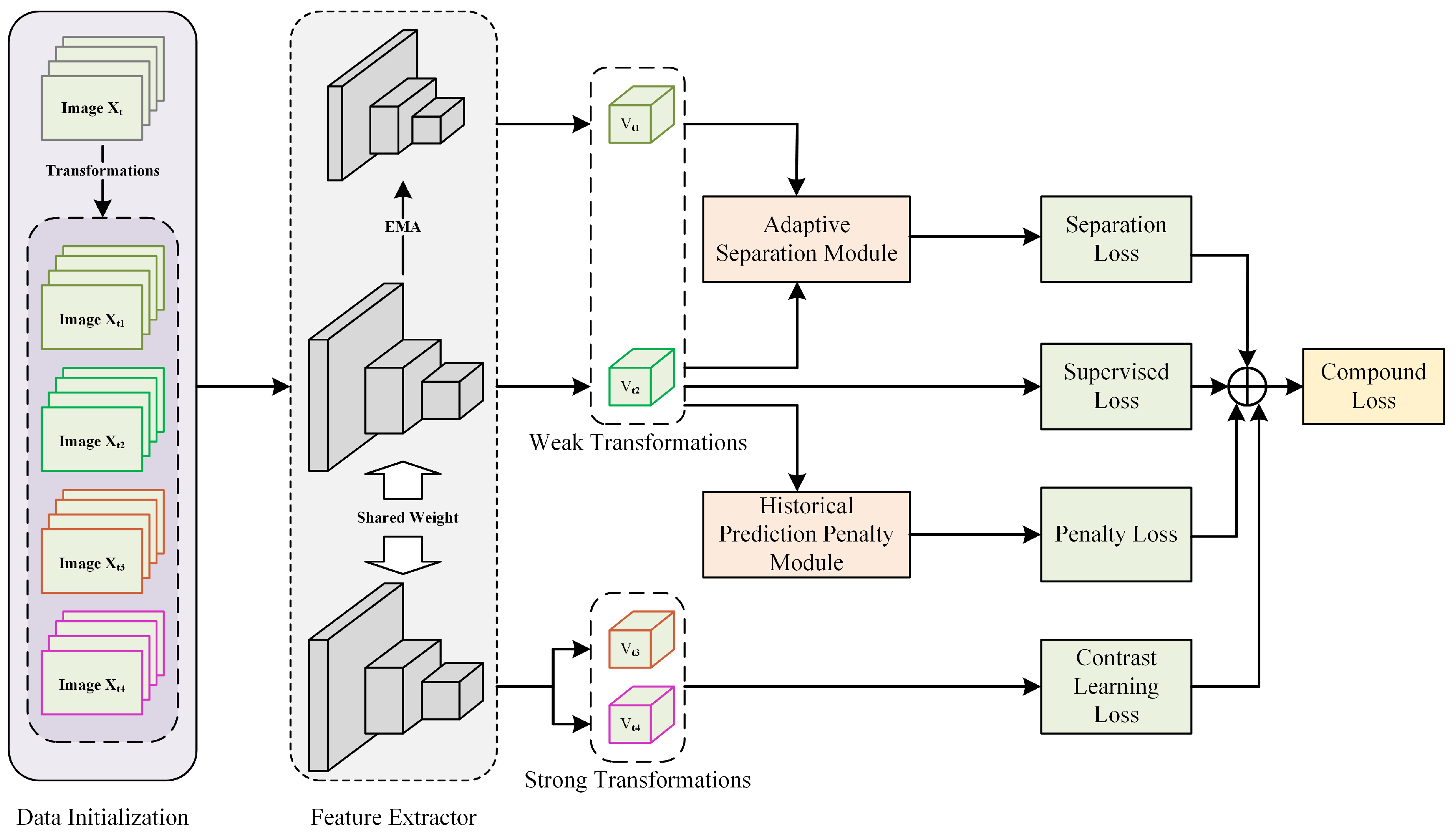
As a branch of self-supervised learning, contrastive learning aims to derive general representations from data without any human-annotated labels [52]. By leveraging an unsupervised training approach, contrastive learning benefits all downstream tasks [53]. Recent studies have introduced various contrastive learning regularization functions and architectures. MoCo [54] utilizes a memory bank to build a dynamic dictionary and introduces the use of a momentum encoder to maintain a large and consistent dictionary of visual representations. SimSiam [19] and SimCLR [55], with their end-to-end training frameworks, further demonstrate that nonlinear projection heads can enhance feature representation. BYOL [56] strengthens disturbance consistency between different views by using a target network and a slowly moving average of the online network, preventing model collapse. These methods focus on learning self-supervised representations without labels. The advantage of using contrastive learning for noisy labels is that it allows for constructing a low-dimensional feature embedding space without relying on professional medical annotations, effectively preserving the structural similarities of the original dataset. Some recent approaches [57,58] used contrastive representation learning to address the noise label problem. Compared with these methods, our focus is more on solving the fundamental issue of preventing noisy labels from dominating the learning of representations.

3. Method

3.1. Problem Setting

Traditional pathological image classification tasks are supervised, aiming to identify an optimal mapping function $\mathcal{F}(·;\theta )$ that closely associates a given image space X with a label space Y. The training set ${D\left(X_i,Y_i\right)}_{i=1}^N$ consists of images annotated by multiple experts. Each sample $\left(X_i,Y_i\right)$ is independently and identically distributed, with N denoting the number of training samples. The goal is to minimize empirical risk, thus optimizing the classifier:

$$\mathcal{F}(·;\theta )=\underset{\theta }{argmin}\sum _{\left(X_i,y_i\right)\in D_{train}}\mathcal{L}({\mathcal{Y}}_i,\mathcal{F}(X_i,\theta ))$$

(1)

where L represents the true loss function and $\mathcal{F}(x_i;\theta )$ is the predicted label for $x_i$. However, in pathological image classification tasks, noisy labels invariably exist in various forms. Specifically, we are provided with a noisy training dataset ${\tilde{D}}_{train}={({\mathcal{X}}_i,{\tilde{\mathcal{Y}}}_i)}_{i=1}^N$ where ${\tilde{\mathcal{Y}}}_i$ represents the noisy label. The true ground truth labels $\mathcal{Y}$, due to various reasons, are either inaccessible or inconsistent. Even when simulating such noisy training datasets, we assumed that the ground truth labels were unavailable. The presence of noisy labels makes the training process for an optimal classifier unreliable, aiming for the minimal expected risk. In this scenario, our objective was to design a noise-resistant training framework, enabling a neural network trained on the noisy dataset $\tilde{\mathcal{D}}$ to achieve performance comparable to one trained on $\mathcal{D}$.

3.2. Method Framework

To alleviate the propagation of noisy labels during network training, we integrated contrastive learning methods which do not involve image label supervision. Since no image labels were involved, we could utilize all training data to obtain noise-independent visual representations. Meanwhile, we used a historical prediction consistency strategy to reduce the model’s memorization of noisy labels in later stages, providing more stable “clean” features for subsequently separated samples. The module’s construction is described in Section 3.5. In addition, we also designed an adaptive separation module to further dynamically separate noisy samples from clean samples and use different learning methods for different samples. This part is described in Section 3.6. Our proposed method’s training framework is shown in Figure 1. It is worth noting that our method’s framework is straightforward to implement and does not require any prior knowledge, such as the noise ratio, data distribution, or additional clean samples. The technical details are described in the following sections.

3.3. Data Initialization

Each sample $X_i$ is transformed into four samples ($X_{i_1}$, $X_{i_2}$, $X_{i_3}$, and $X_{i_4}$) through different image augmentation combinations. Specifically, $X_{i_1}$ and $X_{i_2}$ are weakly augmented images obtained through basic transformations, including rotation and vertical and horizontal flipping, with a 50% probability. Meanwhile, $X_{i_3}$ and $X_{i_4}$ are strongly augmented versions based on weak augmentations and some pixel value transformations. With a 50% probability, Gaussian blurring, color, and grayscale jittering were applied. It is worth noting that color jittering was only used for three-channel pathological images, while grayscale jittering was used for single-channel pathological images. To avoid the loss of meaningful pathological content, we did not use random cropping or erasing operations. Here, $X_{i_1}$ and $X_{i_2}$ were fed into the feature extractor and distillation feature extractor, obtaining $V_{i_1}$ and $V_{i_2}$, respectively, for subsequent module computations and supervised loss calculations, while $X_{i_3}$ and $X_{i_4}$ were fed into the feature extractor, obtaining $V_{i_3}$ and $V_{i_4}$, respectively, for contrastive learning loss computation.

3.4. Contrastive Learning Feature Extractor

Contrastive learning is a self-supervised method that does not require additional labels or specialized architectures [18]. The consensus in this self-supervised method is that different views and transformations of the same image should have the same label. We refer to the commonly used contrastive learning method SimSiam [19], where the high-dimensional features $V_{i_3}$ and $V_{i_4}$ extracted by the feature extractor are mapped through an MLP to low-dimensional features $U_{i_3}$ and $U_{i_4}$, respectively. The intrinsic similarity between $U_{i_4}$ and $U_{i_3}$ can then be represented by the cosine similarity between their corresponding low-dimensional space features:

$$\mathcal{L}({\mathcal{U}}_{{\mathrm{i}}_3},{\mathcal{U}}_{{\mathrm{i}}_4})=\frac{{\mathcal{U}}_{{\mathrm{i}}_3}·{\mathcal{U}}_{{\mathrm{i}}_4}}{\max \left(\right|\left|{\mathcal{U}}_{{\mathrm{i}}_3}\right|{|}_2·\left|\right|{\mathcal{U}}_{{\mathrm{i}}_4}|{|}_2,ϵ)}$$

(2)

where $ϵ$ is a smaller value to avoid division by zero. The default value was 1 $\times {10}^{-8}$. Contrastive learning was guided by the intrinsic similarity loss defined below:

$${\mathcal{L}}_c=\sum _{i=1}^N(\mathcal{L}({\mathcal{U}}_{i_3},{\mathcal{U}}_{i_4})+\mathcal{L}({\mathcal{U}}_{i_4},{\mathcal{U}}_{i_3}))$$

(3)

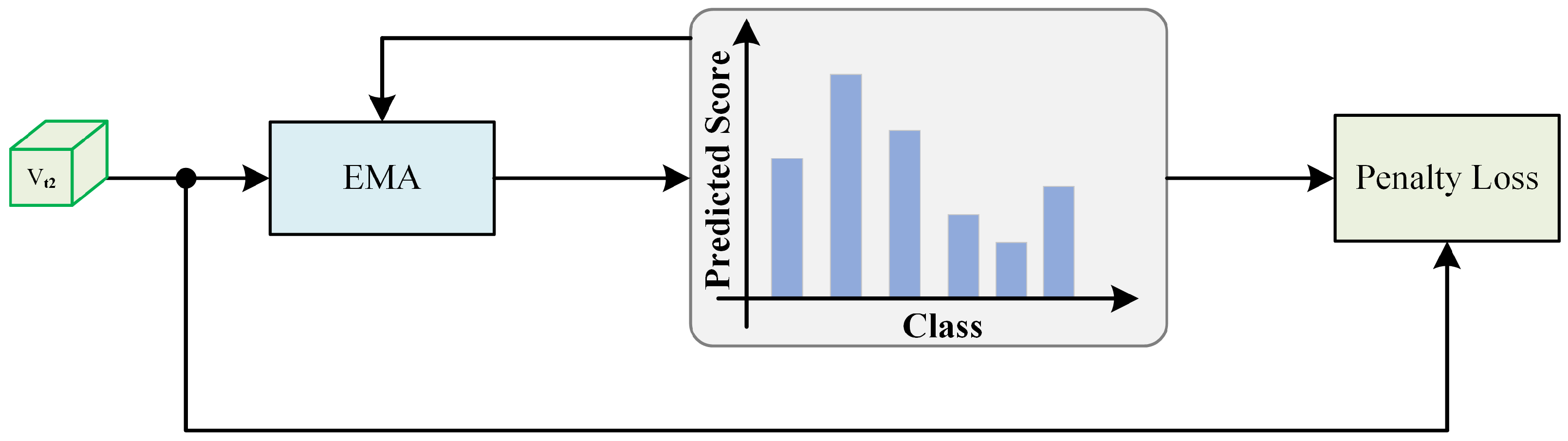
3.5. Historical Prediction Penalty Module

During the further training process, we observed a gradual shift from training dominated by clean labels to training dominated by noisy labels. However, during this transition, the model’s predictions for data samples showed a relatively noticeable change. To counteract the dominance of noisy labels in the training process, we propose a historical prediction penalty module (HPPM), as shown in Figure 2. We suggest that the model’s predictions should maintain more similarity to its previous predictions. In other words, we allow differences, but these differences should not be too significant. In practice, we reassess the category of each sample at every iteration of the model. The estimation for the $i^{th}$ sample after the $k^{th}$ round of training is as follows:

$$p_{k_i}=\left(1-m\right)\ast q_{k_i}+m\ast p_{k-1_i}$$

(4)

where m is a constant, p is initialized as the probability from the first prediction after the warm-up phase ends, and q represents the current prediction result. We combined the prediction with the model’s current prediction for the sample using the cross-entropy function, resulting in the following loss function:

$${\mathcal{L}}_h(p,q)=-\sum _{x}p\left(x\right)logq\left(x\right)$$

(5)

This approach ensures that despite allowing for some degree of prediction variation, the divergence remained within a manageable range, mitigating the impact of noisy labels on the training process.

3.6. Adaptive Separation Module

The historical prediction consistency regularization can only guide the model’s predictions to avoid drastic changes, but it is insufficient to prevent the model from memorizing noisy labels in the later stages. In other words, during the later stages of training, the model’s training is still dominated by noisy labels. However, we must note that during the early and middle stages of training, we put in a lot of effort to mitigate the impact of noisy labels on the model’s performance. Therefore, we hope to use an implicit sample selection strategy during this training period to filter out clean and noisy samples as much as possible. Consequently, we propose an adaptive separation module (ASM), as shown in Figure 3. The design idea of this module was inspired by the recently popular knowledge distillation architecture. In the ASM module, we first use the recently popular knowledge distillation architecture to obtain feature pairs and use distillation loss to bring features of the same image closer together while pushing features of different images apart. On this basis, we added a filter to separate noisy data from clean data. We obtained the teacher network by applying an exponential moving average (EMA) to the student network model’s parameters:

$${\theta }_{t_i}=m\ast {\theta }_{s_i}+(1-m)\ast {\theta }_{t_{i-1}}$$

(6)

where ${\theta }_{s_i}$ represents the parameters of the student network model in the ith round and ${\theta }_{t_i}$ represents the parameters of the teacher network model in the ith round, while m is a constant. To better align the teacher and student network models, their similarity was measured by the knowledge distillation loss proposed in previous work:

$${\mathcal{L}}_{kd}=-\frac{1}{N}\sum _i^N{P}_{ti}log{P}_{si}$$

(7)

$P_{ti}$ is the prediction made by the teacher network model for sample i, and $P_{si}$ is the prediction made by the student network model for sample i. We believe that the predictions of the student and teacher network models for the same sample should maintain similar characteristics. Therefore, we used KL divergence to measure the distance between the predictions of the student and teacher network models:

$$D_{\mathrm{kl}}(P_s\parallel P_t)=\sum _i{P}_s\left(i\right)ln\frac{P_s\left(i\right)}{P_t\left(i\right)}$$

(8)

We considered samples with close prediction distances to be clean labels, while samples with large prediction distances were considered noisy label samples. In other words, we set a distance threshold $\mu$. If $D_{\mathrm{kl}}(p_{si},p_{ti})<\mu$, then $({\mathcal{X}}_i,{\tilde{\mathcal{Y}}}_i)$ was a clean sample, and ${\tilde{\mathcal{Y}}}_i={\mathcal{Y}}_i$. Otherwise, it was a noisy sample. For different samples, we used different learning methods. For clean samples, we used the effective cross-entropy function as the supervised learning loss for classification:

$${\mathcal{L}}_s(x_i,y_i)=CE(\mathcal{F}(x_i,\theta ),y_i)$$

(9)

For noisy samples, we used an evenly distributed probability across all classes except the current class as the new label $y_j^{\prime }$. We call this the negative learning loss. This loss function is described as follows:

$$y_j^{\prime }={\left[\frac{1}{C-1},\frac{1}{C-1},\cdots ,0,\cdots \frac{1}{C-1},\right]}^C$$

(10)

$${\mathcal{L}}_n(x_j,y_j^{\prime })=\sum _{j=1}^C{y}_j^{\prime }log\left(p_{x_j}\right)$$

(11)

Among Equation (9), the jth one is 0, and the rest are all $\frac{1}{C-1}$. However, during the training process, the student network model and the teacher model will gradually become more similar, and thus a fixed threshold $\mu$ is obviously not able to distinguish between samples particularly well. We hope to use an adaptive threshold $\mu$ that can adjust according to the model’s training process, where $\mu =(ma{x}_{epoch}/no{w}_{epoch})\ast \mu$. The initial value of $\mu$ was set to 0.5. Finally, the entire ASM network model was jointly updated through the various loss functions:

$$L_a=\left\{\begin{array}{cc}{L}_{kd}+L_s,\hfill & if:D_{\mathrm{kl}}(p_{si},p_{ti})<\mu \hfill \\ L_{kd}+L_n,\hfill & if:D_{\mathrm{kl}}(p_{si},p_{ti})\ge \mu \hfill \end{array}\right.$$

(12)

3.7. Overall Loss Functions

Our proposed method utilizes a combination of four different types of composite loss functions: the contrastive learning loss $L_c$, the supervised loss $L_s$, the historical prediction penalty loss $L_h$, and the adaptive separation loss $L_a$. In the first stage, which is the warm-up stage, the contrastive loss function and the supervised loss function with a small weight are mainly used to update the feature extractor. The loss function $L_{stage1}$ in the first stage is expressed in the formula X. In this stage, the network model will deeply mine the intrinsic similarity between each sample in the entire dataset, and due to the introduction of the small-weight supervised loss, the samples will move closer to the class while maintaining similarity, further enhancing the stability of the feature extractor and impeding the learning of noisy samples. In the second stage, in addition to the contrastive learning loss and supervised loss, the HPPM and ASM are further added to reinforce supervised learning, which is conducive to impeding the model’s learning of noisy label samples in the later stages, obtaining a noise-tolerant training framework. More specifically, the HPPM and ASM, together with the supervised learning loss function, play a dominant role, while $L_c$ can be considered a regularization variable for the entire training process. Therefore, the loss function $L_{stage2}$ is summarized as the formula X + 1:

$${\mathcal{L}}_{stage1}={\mathcal{L}}_c+{\lambda }_1\ast {\mathcal{L}}_s$$

(13)

$${\mathcal{L}}_{stage2}={\mathcal{L}}_s+{\lambda }_2\ast ({\mathcal{L}}_h+{\mathcal{L}}_a+{\lambda }_1\ast {\mathcal{L}}_c)$$

(14)

where ${\lambda }_1$ is a small weight coefficient set to 0.1 and ${\lambda }_2$ is a hyperparameter representing the regularization strength.

4. Experiment Design

4.1. Dataset Accumulation and Transformation

4.1.1. Dataset Description

In this study, we evaluated our method using two publicly available pathological datasets: PatchCamelyon [59] and Chaoyang [40]. PatchCamelyon, part of the Camelyon16 challenge, includes 400 H&E-stained whole slide images (WSIs) of lymph node sections from breast tumor cases. These slides were obtained and digitized at two centers with a 40× objective, achieving a pixel resolution of 0.243 $\mathsf{\mu }$m. The dataset ensures no duplicate WSIs across different splits, maintaining a 50/50 balance between positive and negative samples. It comprises 327,680 color images (96 px × 96 px) extracted from tissue scans. Each image is labeled with a binary indicator for metastatic tissue. We selected 32,766 samples from PatchCamelyon and split them into training, test, and validation sets at an 8:1:1 ratio, resulting in 26,214, 3276, and 3276 samples, respectively.

Chaoyang [40] is a four-class colon pathology slide dataset with patches 512 px × 512 px in size. Three colon pathology experts from Beijing Chaoyang Hospital labeled the lesions. We used samples consistently annotated by all three experts for the test set, while the remaining samples formed the training set. The Chaoyang dataset consists of 4021 training samples and 2139 test samples, with the training set including 1111 normal, 842 serrated, 1404 adenocarcinoma, and 664 adenoma samples. The test set contains 705 normal, 321 serrated, 840 adenocarcinoma, and 273 adenoma samples. This dataset was created from real-world scenarios.

4.1.2. Noise Injection

To simulate the noisy label situation on the lymph node dataset we used, we randomly selected a percentage $\rho \in \left[0.05,0.10,0.20,0.30,0.40\right]$ of images from each class and flipped their labels, following common practices. Through this process, we obtained a noisy training dataset containing a certain amount of incorrectly labeled images. Noisy labels were defined as $P(\tilde{y}=k\left|y=j\right)={\rho }_j,k\ne j$ and $P(\tilde{y}=j\left|y=j\right)=1-{\rho }_j$. Here, $\tilde{y}$ represents the corrupted noisy label, and y represents the clean label. We used accuracy as the evaluation metric. In our work, we evaluated the robustness of our method under various noise rates, from low noise to high noise. Referring to the real-world noise rate in pathological datasets and a previous work [40], for all synthesized noisy datasets, we simulated five noise rates from 0% to 40%, with a step size of 10%. To better reflect the low noise rate in pathological images, we added a 5% noise rate scenario. The noise rate was set to not exceed 40%, as we believe that discussing high-noise scenarios in rigorous pathological image datasets is meaningless.

4.2. Evaluation Metrics

Our method was evaluated using four metrics: accuracy (ACC), precision, recall, and F1 score. The definitions of these metrics are provided below:

$$\mathrm{ACC}=\frac{\mathrm{TP}+\mathrm{TN}}{\mathrm{TP}+\mathrm{TN}+\mathrm{FP}+\mathrm{FN}}$$

(15)

$$Precision=\frac{\mathrm{TP}}{\mathrm{TP}+\mathrm{FP}}$$

(16)

$$\mathrm{Recall}=\frac{\mathrm{TP}}{\mathrm{TP}+\mathrm{FN}}$$

(17)

$$\mathrm{F}1\mathrm{Score}=\frac{2\ast \mathrm{Precision}\ast \mathrm{Recall}}{\mathrm{Precision}+\mathrm{Recall}}$$

(18)

Here, TP, TN, FP, and FN represent true positive, true negative, false positive, and false negative, respectively. These metrics are applicable to binary classification problems. For multiclass tasks, each metric is calculated for every class and then averaged using the macro-average method.

4.3. Compared Methods

To demonstrate the effectiveness of our approach, we conducted comparisons with recent state-of-the-art methods in the field of learning with noisy labels, as well as a baseline scenario without any robust techniques. The methods selected for comparison included the following:

(1)

Standard: This baseline involves training a common convolutional neural network (CNN) without noise-handling techniques.

(2)

Joint [22]: This method proposes a simultaneous update of network parameters and data labels to tackle the issue of noisy labels.

(3)

Co-teaching [5]: Introduces a dual-network architecture where each network selects samples with smaller loss for the other network’s training and parameter updating.

(4)

DivideMix [11]: This method proposes a novel framework for learning with noisy labels using semi-supervised learning techniques.To achieve noise robustness, it trains two networks concurrently through dataset co-partitioning, label co-refinement, and co-guessing.

(5)

Co-Correcting [46]: This offers a noise-resistant medical image classification framework which enhances accuracy through dual-network mutual learning, label probability estimation, and curricular label correction.

(6)

HSA_NRL [40]: This method uses the training prediction history to distinguish between hard and noisy samples. This robust learning method for histopathological image classification aims to preserve more clean samples and improve model performance.

The use of convolutional neural networks (CNNs) instead of Kalman filters (KFs) or decision trees (DTs) for pathological image classification is preferred because CNNs excel in automatic feature extraction, effectively handle complex and variable image data, have good generalization capabilities, and offer flexible architectures that can be adjusted according to the task. A KF is better suited for real-time linear estimation tasks, and DTs perform poorly with high-dimensional complex data like medical images.

Experiments were conducted using the original authors’ codes for a fair comparison. Due to GPU memory limitations, the patch size was set to 64 when testing DivideMix on the PatchCamelyon dataset.

4.4. Implementation Details

We employed DenseNet121 as our backbone network, which is a commonly used architecture suitable for classification tasks, for all experiments on breast lymphoma and colon tumor datasets. The training utilized an SGD optimizer with an initial learning rate of 0.01 and momentum of 0.9. Details regarding the training batch size and learning rate decay during the training process are presented in

Table 1. The key hyperparameter used in training for each task in our experiments.

Dataset	Pre-Training Epoch	Batch Size	Optimizer	${\mathit{\lambda }}_1$	${\mathit{\lambda }}_2$
Chaoyang	30	64	SGD	0.1	2
PatchCamelyon	50	128	SGD	0.1	2

. All experiments were conducted in a software environment of Ubuntu-20.04 and Pytorch 1.12.1, with hardware comprising an Intel(R) Xeon(R) Gold 5218R CPU @ 2.10 GHz, NVIDIA RTX3090 GPU, and 24 GB of RAM.

5. Results and Discussion

5.1. Classification Experiment Results for Synthetic Noisy Medical Data

This section introduces the experimental results of our method on the synthetic noisy tumor dataset PatchCamelyon.

Table 2. Results for the PatchCamelyon dataset with different noise levels (accuracy (%)).

Noise Ratio	Clean	0.05	0.10	0.20	0.30	0.40
Standard	86.64	84.44	81.69	74.24	67.10	58.46
Joint Optim	36.18	45.07	38.37	39.95	38.74	36.44
Co-Teaching	74.85	74.54	74.40	73.40	76.84	67.97
DivideMix	84.85	83.84	83.43	80.11	62.40	42.49
Co-Correcting	86.98	85.66	87.25	87.14	87.10	84.95
HSA-NRL	93.83	92.09	93.13	87.33	85.99	82.94
Ours	94.69	94.35	93.41	91.27	88.46	85.07

shows our method’s and other competitors’ results for the lymph node tumor classification task.

Our method achieved better results for the clean dataset than the cross-entropy loss. However, for all noise rates, Joint Optim performed even worse than the standard method without robustness. We believe that the training strategy of jointly updating network parameters and labels may not be effective in the medical image domain. For noisy label datasets, HAS-NRL and our method significantly outperformed the other methods, indicating that the dual-network training strategy with model self-distillation can alleviate bias in sample selection. Furthermore, our method outperformed HAS-NRL in all noise settings, showing that adding historical prediction and unsupervised regularization losses can lead to learning more robust feature representations. For small noise ratio settings, the overfitting on noisy labels was not as severe as it was for severely corrupted datasets, and our method achieved the best results.

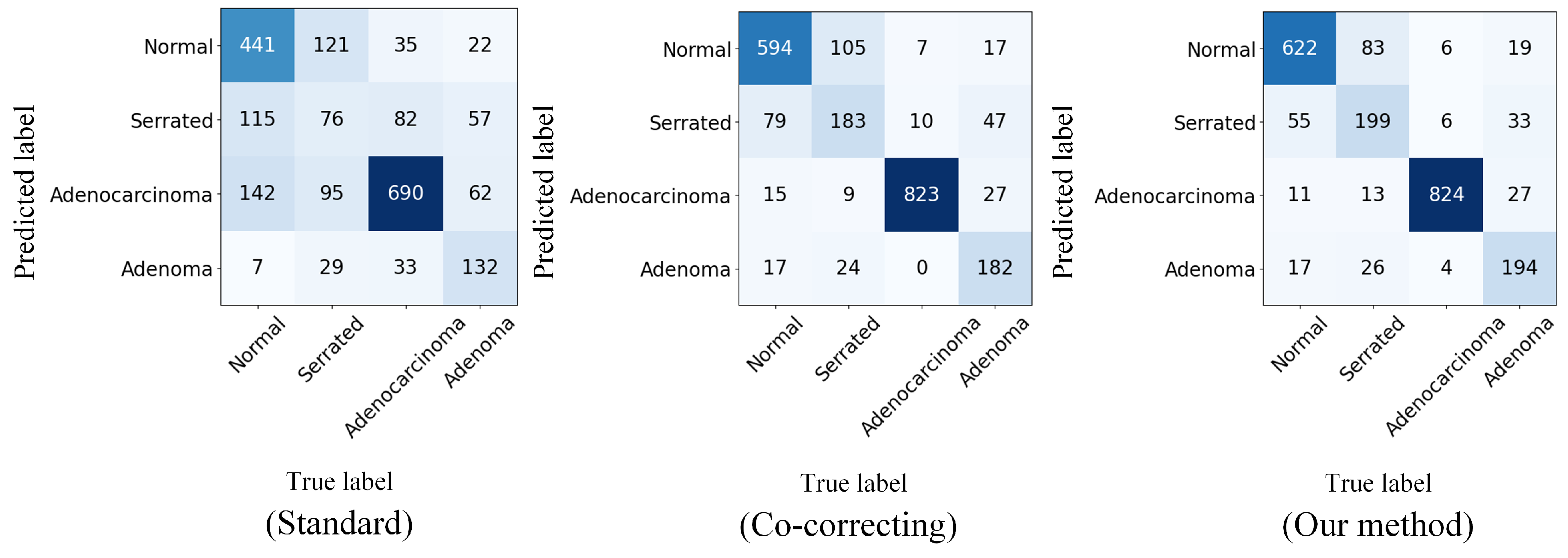
5.2. Classification Experiment Results for Real-World Noisy Medical Data

In addition to manually added noise, we further evaluated the generalization and robustness of our method on the real-world tumor image dataset Chaoyang. Training details can be found in the Implementation Details subsection. It is worth noting that, to be consistent with the previous experiments, we used the same threshold $\mu$ as the one for the synthetic noise. We conducted experiments on different methods. The test performance is shown in

Table 3. Results for the Chaoyang dataset with a real-world noise level.

Methods	ACC	Precision	Recall	F1 Score
Standard	62.60	57.42	55.76	54.18
Joint Optim	75.99	70.97	67.91	67.72
Co-teaching	79.39	74.57	70.77	71.97
DivideMix	77.25	70.68	69.11	69.78
Co-Correcting	83.31	76.48	78.87	77.61
HSA-NRL	83.40	78.33	75.45	76.54
Ours	85.97	79.84	81.95	80.88

. On this dataset, our method achieved state-of-the-art performance. We can conclude that our method can flexibly work on real-world noisy datasets without any prior knowledge.

Figure 4 shows the confusion matrix visualization we computed on the real-world noisy dataset Chaoyang. The confusion matrix is a common tool for evaluating the performance of classification models. It can display the model’s predictions for each class, including correctly classified samples and misclassification confusion.

From the confusion matrix of the standard method, we can see that without adding any robustness, the DNNs had rather limited performance in classifying noisy-labeled pathology images. After incorporating the noise-resistant dual-network prediction, the confusion matrix of Co-Correcting significantly improved the classification performance for each class. The confusion matrix of our method demonstrates the classification effect of our method. We further optimized the performance. Compared with previous methods, our method significantly improved the classification ability for the normal class, reducing the confusion probability between the normal, serrated, and adenocarcinoma classes and thereby achieving an overall performance improvement.

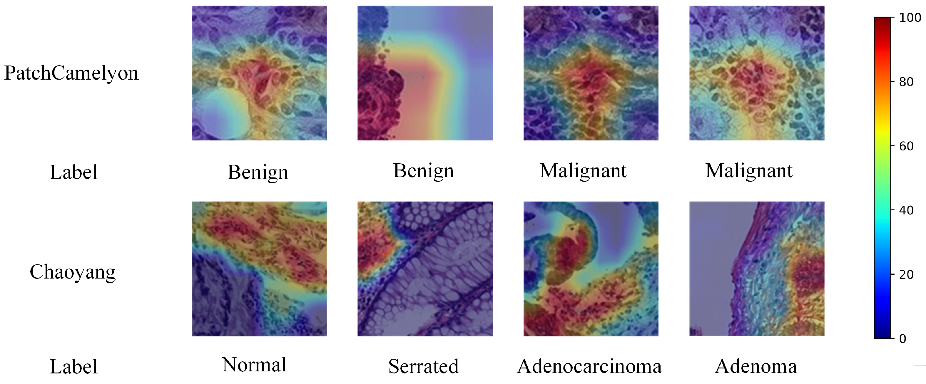
5.3. Grad-CAM Visualization

We used Grad-CAM [60] for qualitative evaluation of our proposed method, with the visualization results shown in Figure 5. These results include CAM visualization examples from both the PatchCamelyon and Chaoyang datasets. For PatchCamelyon, a malignant label signifies that at least one tumor pixel is present in a patch’s the central 32 × 32 pixel region. In the Chaoyang dataset, the boundaries of tumor tissues are delineated, aiding in diagnosis. Grad-CAM heatmaps use warmer colors to indicate areas of higher model attention and cooler colors for areas of lower attention. The visualizations demonstrate that our model accurately focused on tumor and lesion locations. This experiment confirms that our model effectively learns crucial features even with noisy label data, enhancing future computer-aided pathological diagnosis systems. Training with noisy-labeled data helps the model adapt to real-world noise and uncertainty, improving robustness and reliability. Furthermore, our method showed consistent performance across different types of tumors, highlighting its versatility. These results suggest that integrating such techniques into clinical workflows can significantly aid pathologists in making more accurate diagnoses.

5.4. Backbone Ablation Study

We conducted ablation studies on the PatchCamelyon dataset with different backbone networks at various noise rates. As can be seen in

Table 4. Classification accuracy (%) with different backbones in the PatchCamelyon datasets.

Noise Ratio	Clean	0.05	0.10	0.20	0.30	0.40
ResNet18	94.14	92.80	91.85	88.37	85.65	81.44
ResNet34	94.72	93.56	92.77	92.00	86.90	85.53
ResNet50	94.17	93.59	92.74	88.64	86.78	81.93
DenseNet121	94.69	94.35	93.41	91.27	88.46	85.07
DenseNet161	95.27	94.35	93.40	91.27	87.30	82.72

Note: The bolded text is the best classification accuracy in Table 4, Table 5 and Table 6.

, for any backbone network, the accuracy of all models decreased as the noise rate increased because noisy labels interfered with the model, increasing the difficulty of the classification task. It can be observed that DenseNet121 showed better performance at noise levels of 0.05, 0.10, and 0.30. At the 0.20 and 0.40 noise levels, ResNet34 had better classification results. At a noise level of zero, DenseNet161 outperformed DenseNet121. In summary, the performance of the DenseNet series of models was better than that of the ResNet series of models. This may be due to the unique structural design of the DenseNet series of models, where each layer is connected to all previous layers. This design helps maintain gradient flow within the network, reducing information loss and thus typically achieving better performance in image classification tasks. After careful consideration, in all experimental settings of this paper, we adopted DenseNet121 as the backbone network of our model.

5.5. Module Ablation Study

To better understand the importance of each component in our proposed method, we conducted performance validations on the PatchCamelyon and Chaoyang datasets using a leave-one-out approach.

Table 5. Classification accuracy (%) of the model when using different components.

HPPM	ASM	CLM	Clean	0.05	0.10	0.20	0.30	0.40	Real World
×	×	×	86.64	84.44	81.69	74.24	67.10	58.46	62.60
✓	×	×	93.44	91.03	90.23	88.61	85.50	81.56	85.51
×	✓	×	94.84	93.96	93.22	90.63	87.09	83.46	85.32
✓	✓	×	95.09	93.93	93.35	90.60	87.64	83.27	85.56
✓	×	✓	92.92	92.00	91.23	87.70	84.92	81.53	85.46
×	✓	✓	94.68	93.96	93.19	91.45	87.36	81.84	85.74
✓	✓	✓	94.69	94.35	93.41	91.27	88.46	85.07	85.97

presents the ablation study of various components, including the historical prediction penalization module (HPPM) with different noise ratios, the adaptive separation module (ASM), and the contrastive learning module (CLM). Notably, as a branch of self-supervised learning techniques, the CLM enhances the visual representation of DNNs but does not independently output prediction labels.

As shown in Table 5, the impact of each module was not all that apparent under low noise conditions. However, their combined effect significantly improved the performance at higher noise levels. The first three rows reveal that using the HPPM or ASM alone significantly enhanced the model’s classification performance. The HPPM, by constraining the model to fit noise labels, did not eliminate a substantial number of noisy label samples in the training set, leading to the model’s memorization of noise labels in later training stages and resulting in mediocre performance at higher noise rates. Conversely, the combined use of the three components further elevated model performance. This improvement was due to the progressive training process we designed, where the HPPM and CLM prepare data samples in the ASM for better differentiation, effectively segregating noisy samples.

5.6. Hyperparameter Experiment

To investigate the impact of the regularization coefficient ${\lambda }_2$ on the model performance, we conducted hyperparameter comparison experiments on the synthetic noise dataset PatchCamelyon and the real-world noise dataset Chaoyang.

The results, as shown in

Table 6. Classification accuracy (%) with regularization factor ${\lambda }_2$ in the PatchCamelyon and Chaoyang datasets.

${\mathit{\lambda }}_2$	Clean	0.05	0.10	0.20	0.30	0.40	Real World
0.1	93.83	92.46	90.93	88.98	86.14	81.62	85.83
1	94.51	93.71	92.16	90.57	87.42	84.86	85.60
2	94.69	94.35	93.41	91.27	88.46	85.07	85.97
5	95.36	94.20	93.25	91.03	87.55	81.62	85.41
10	95.24	93.71	93.32	92.31	88.13	80.65	85.27
100	93.07	93.16	92.64	91.39	87.52	80.80	84.67

, indicate that our method achieved optimal performance mostly when ${\lambda }_2$ = 2. Specifically, the best performance on the synthetic noise dataset PatchCamelyon at a label noise rate of 0.2 was obtained when ${\lambda }_2$ = 10. However, when the noise rate increased to 0.4, a regularization coefficient of ${\lambda }_2$ = 10 significantly impaired the model’s performance. Overall, when ${\lambda }_2$ = 100, the excessive regularization strength made the model focus more on the relationships between data features, weakening the learning from labels and resulting in underfitting. Considering these findings comprehensively, we fixed ${\lambda }_2$ at two for all experiments in this study.

6. Conclusions

In this paper, we proposed a novel self-supervised joint regularization approach that effectively mitigates the adverse effects of noisy labels in pathological image classification. This method is based on a structured process that comprises enhanced feature extraction, noise fitting suppression, and noise sample separation. To alleviate overfitting to noisy labels during the network model’s training, we introduced the historical prediction penalty module, which controls the similarity of model predictions across adjacent epochs, thus reducing the model’s overfitting to labels. Finally, to further improve the model’s classification performance, we proposed the adaptive separation module, which uses a knowledge distillation approach to bring samples closer together and then adaptively separates the more distant sample data, mitigating the impact of noisy labels. The experimental findings indicate that our approach surpassed existing state-of-the-art techniques in managing noisy labels across both synthetic and real-world datasets. Notably, on the Chaoyang pathological image dataset, our method achieved a 2.57% improvement in classification accuracy. Additionally, our approach does not require any prior information, such as noise rates or a clean validation set. This further illustrates our method’s capability to handle noisy labels in real-world pathological image classification applications. In this paper, we addressed the issue of noisy labels in class-balanced pathological datasets. However, in practical applications, the number of positive samples in pathological datasets is much lower than that of negative samples, making the issue of class imbalance more significant. Addressing noisy labels in class-imbalanced datasets will be the focus of our future work.

References

1. Zhang, C.; Bengio, S.; Hardt, M.; Recht, B.; Vinyals, O. Understanding deep learning (still) requires rethinking generalization. Commun. ACM 2021, 64, 107–115. [Google Scholar] [CrossRef]
2. Cheng, H.; Zhu, Z.; Sun, X.; Liu, Y. Mitigating Memorization of Noisy Labels via Regularization between Representations. In Proceedings of the International Conference on Learning Representations (ICLR), Kigali, Rwanda, 1–5 May 2023; pp. 1–27. [Google Scholar]
3. Arplt, D.; Jastrzbskl, S.; Bailas, N.; Krueger, D.; Bengio, E.; Kanwal, M.S.; Maharaj, T.; Fischer, A.; Courville, A.; Benglo, Y.; et al. A closer look at memorization in deep networks. In Proceedings of the International Conference on Machine Learning (ICML), Sydney, Australia, 6–11 August 2017; Volume 1, pp. 350–359. [Google Scholar]
4. Huang, C.; Wang, W.; Zhang, X.; Wang, S.H.; Zhang, Y.D. Tuberculosis Diagnosis Using Deep Transferred EfficientNet. IEEE/ACM Trans. Comput. Biol. Bioinform. 2023, 20, 2639–2646. [Google Scholar] [CrossRef] [PubMed]
5. Han, B.; Yao, Q.; Yu, X.; Niu, G.; Xu, M.; Hu, W.; Tsang, I.; Sugiyama, M. Co-teaching: Robust training of deep neural networks with extremely noisy labels. In Proceedings of the 32nd International Confonference on Neural Information Processing Systems (NIPS), Montreal, QC, Canada, 3–8 December 2018; Volume 31, pp. 1–11. [Google Scholar]
6. Yu, X.; Han, B.; Yao, J.; Niu, G.; Tsang, I.W.; Sugiyama, M. How does disagreement help generalization against label corruption? In Proceedings of the International Conference on Machine Learning (ICML), Long Beach, CA, USA, 10–15 June 2019; pp. 12407–12417. [Google Scholar]
7. Nguyen, D.T.; Mummadi, C.K.; Nhung Ngo, T.P.; Phuong Nguyen, T.H.; Beggel, L.; Brox, T. Self: Learning to Filter Noisy Labels with Self-Ensembling. In Proceedings of the International Conference on Learning Representations (ICLR), Addis Ababa, Ethiopia, 26–30 April 2020; pp. 1–16. [Google Scholar]
8. Wei, H.; Feng, L.; Chen, X.; An, B. Combating Noisy Labels by Agreement: A Joint Training Method with Co-Regularization. In Proceedings of the Conference on Computer Vision and Pattern Recognition (CVPR), Virtual, 18–24 June 2020; pp. 13723–13732. [Google Scholar]
9. Han, G.; Guo, W.; Zhang, H.; Jin, J.; Gan, X.; Zhao, X. Sample self-selection using dual teacher networks for pathological image classification with noisy labels. Comput. Biol. Med. 2024, 174, 108489–108501. [Google Scholar] [CrossRef] [PubMed]
10. Fan, H.; Zhang, X.; Xu, Y.; Fang, J.; Zhang, S.; Zhao, X.; Yu, J. Transformer-based multimodal feature enhancement networks for multimodal depression detection integrating video, audio and remote photoplethysmograph signals. Inf. Fusion 2024, 104, 102161. [Google Scholar] [CrossRef]
11. Li, J.; Socher, R.; Hoi, S.C. Dividemix: Learning with Noisy Labels as Semi-Supervised Learning. In Proceedings of the International Conference on Learning Representations (ICLR), Addis Ababa, Ethiopia, 26–30 April 2020; pp. 1–11. [Google Scholar]
12. Pulido, J.V.; Guleria, S.; Ehsan, L.; Fasullo, M.; Lippman, R.; Mutha, P.; Shah, T.; Syed, S.; Brown, D.E. Semi-Supervised Classification of Noisy, Gigapixel Histology Images. In Proceedings of the 20th IEEE International Conference on Bioinformatics and Bioengineering (BIBE), Cincinnati, OH, USA, 26–28 October 2020; pp. 563–568. [Google Scholar]
13. Bdair, T.; Navab, N.; Albarqouni, S. FedPerl: Semi-Supervised Peer Learning for Skin Lesion Classification. In Proceedings of the Medical Image Computing and Computer Assisted Intervention (MICCAI), Strasbourg, France, 27 September–1 October 2021; Volume 12903 LNCS, pp. 336–346. [Google Scholar]
14. Wang, Z.; Jiang, J.; Han, B.; Feng, L.; An, B.; Niu, G.; Long, G. SemiNLL: A Framework of Noisy-Label Learning by Semi-Supervised Learning. arXiv 2022, arXiv:2012.00925. [Google Scholar]
15. Zhang, S.; Yang, Y.; Chen, C.; Zhang, X.; Leng, Q.; Zhao, X. Deep learning-based multimodal emotion recognition from audio, visual, and text modalities: A systematic review of recent advancements and future prospects. Expert Syst. Appl. 2024, 237, 121692. [Google Scholar] [CrossRef]
16. Ren, Z.; Kong, X.; Zhang, Y.; Wang, S. UKSSL: Underlying knowledge based semi-supervised learning for medical image classification. IEEE Open J. Eng. Med. Biol. 2023, 5, 459–466. [Google Scholar] [CrossRef] [PubMed]
17. Zhang, S.; Zhang, X.; Zhao, X.; Fang, J.; Niu, M.; Zhao, Z.; Yu, J.; Tian, Q. MTDAN: A Lightweight Multi-Scale Temporal Difference Attention Networks for Automated Video Depression Detection. IEEE Trans. Affective Comput. 2023; early access. [Google Scholar]
18. Dgani, Y.; Greenspan, H.; Goldberger, J. Training a neural network based on unreliable human annotation of medical images. In Proceedings of the IEEE 15th International Symposium on Biomedical Imaging (ISBI), Washington, DC, USA, 4–7 April 2018; pp. 39–42. [Google Scholar]
19. Chen, X.; He, K. Exploring simple Siamese representation learning. In Proceedings of the IEEE/CVF Conference on Computer Vision and Pattern Recognition (CVPR), Virtual, 19–25 June 2021; pp. 15745–15753. [Google Scholar]
20. Arazo, E.; Ortego, D.; Albert, P.; O’Connor, N.E.; McGuinness, K. Unsupervised label noise modeling and loss correction. In Proceedings of the 36th International Conference on Machine Learning (ICML), Long Beach, CA, USA, 9–15 June 2019; Volume 2019, pp. 465–474. [Google Scholar]
21. Miyato, T.; Maeda, S.i.; Koyama, M.; Ishii, S. Virtual adversarial training: A regularization method for supervised and semi-supervised learning. IEEE Trans. Pattern Anal. Mach. Intell. 2018, 41, 1979–1993. [Google Scholar] [CrossRef]
22. Tanaka, D.; Ikami, D.; Yamasaki, T.; Aizawa, K. Joint Optimization Framework for Learning with Noisy Labels. In Proceedings of the IEEE Conference on Computer Vision and Pattern Recognition (CVPR), Salt Lake City, UT, USA, 18–22 June 2018; pp. 5552–5560. [Google Scholar]
23. Patrini, G.; Rozza, A.; Menon, A.K.; Nock, R.; Qu, L. Making deep neural networks robust to label noise: A loss correction approach. In Proceedings of the IEEE Conference on Computer Vision and Pattern Recognition (CVPR), Honolulu, HI, USA, 21–26 July 2017; Volume 2017, pp. 2233–2241. [Google Scholar]
24. Jiang, H.; Gao, M.; Hu, Y.; Ren, Q.; Xie, Z.; Liu, J. Label-noise-tolerant medical image classification via self-attention and self-supervised learning. arXiv 2023, arXiv:2306.09718. [Google Scholar]
25. Tu, Y.; Zhang, B.; Li, Y.; Liu, L.; Li, J.; Zhang, J.; Wang, Y.; Wang, C.; Zhao, C.R. Learning with Noisy Labels via Self-Supervised Adversarial Noisy Masking. In Proceedings of the IEEE/CVF Conference on Computer Vision and Pattern Recognition (CVPR), Vancouver, BC, Canada, 19–22 June 2023; Volume 2023, pp. 16186–16195. [Google Scholar]
26. Tu, Y.; Zhang, B.; Li, Y.; Liu, L.; Li, J.; Wang, Y.; Wang, C.; Zhao, C.R. Learning from Noisy Labels with Decoupled Meta Label Purifier. In Proceedings of the IEEE/CVF Conference on Computer Vision and Pattern Recognition (CVPR), Vancouver, BC, Canada, 19–22 June 2023; Volume 2023, pp. 19934–19943. [Google Scholar]
27. Zheltonozhskii, E.; Baskin, C.; Mendelson, A.; Bronstein, A.M.; Litany, O. Contrast to Divide: Self-Supervised Pre-Training for Learning with Noisy Labels. In Proceedings of the IEEE/CVF Winter Conference on Applications of Computer Vision (WACV), Waikoloa, HI, USA, 4–8 January 2022; pp. 387–397. [Google Scholar]
28. Zhang, J.; Song, B.; Wang, H.; Han, B.; Liu, T.; Liu, L.; Sugiyama, M. BadLabel: A Robust Perspective on Evaluating and Enhancing Label-Noise Learning. IEEE Trans. Pattern Anal. Mach. Intell. 2024, 46, 4398–4409. [Google Scholar] [CrossRef] [PubMed]
29. Karim, N.; Rizve, M.N.; Rahnavard, N.; Mian, A.; Shah, M. UNICON: Combating Label Noise Through Uniform Selection and Contrastive Learning. In Proceedings of the IEEE/CVF Conference on Computer Vision and Pattern Recognition (CVPR), New Orleands, LA, USA, 19–24 June 2022; Volume 2022, pp. 9666–9676. [Google Scholar]
30. Goldberger, J.; Ben-Reuven, E. Training deep neural-networks using a noise adaptation layer. In Proceedings of the International Conference on Learning Representations (ICLR), Toulon, France, 24–26 April 2017; pp. 1–9. [Google Scholar]
31. Tanno, R.; Saeedi, A.; Sankaranarayanan, S.; Alexander, D.C.; Silberman, N. Learning from noisy labels by regularized estimation of annotator confusion. In Proceedings of the IEEE/CVF Conference on Computer Vision and Pattern Recognition (CVPR), Long Beach, CA, USA, 16–20 June 2019; Volume 2019, pp. 11236–11245. [Google Scholar]
32. Xia, X.; Liu, T.; Wang, N.; Han, B.; Gong, C.; Niu, G.; Sugiyama, M. Are anchor points really indispensable in label-noise learning? In Proceedings of the 33rd International Conference on Neural Information Processing Systems (NIPS), Vancouver, BC, Canada, 8–14 December 2019; Volume 32, pp. 1–12. [Google Scholar]
33. Li, S.; Xia, X.; Zhang, H.; Zhan, Y.; Ge, S.; Liu, T. Estimating Noise Transition Matrix with Label Correlations for Noisy Multi-Label Learning. In Proceedings of the 36th International Conference on Neural Information Processing Systems (NIPS), New Orleans, LA, USA, 28 November–9 December 2022; Volume 35, pp. 24184–24198. [Google Scholar]
34. Cheng, D.; Ning, Y.; Wang, N.; Gao, X.; Yang, H.; Du, Y.; Han, B.; Liu, T. Class-dependent label-noise learning with cycle-consistency regularization. In Proceedings of the 36th International Conference on Neural Information Processing Systems (NIPS), New Orleans, LA, USA, 28 November–9 December 2022; Volume 35, pp. 11104–11116. [Google Scholar]
35. Ren, M.; Zeng, W.; Yang, B.; Urtasun, R. Learning to reweight examples for robust deep learning. In Proceedings of the 35th International Conference on Machine Learning (ICML), Stockholm, Sweden, 10–15 July 2018; Volume 10, pp. 6900–6909. [Google Scholar]
36. Liang, X.; Yao, L.; Liu, X.; Zhou, Y. Tripartite: Tackle Noisy Labels by a More Precise Partition. arXiv 2022, arXiv:2202.09579. [Google Scholar]
37. Xiao, R.; Dong, Y.; Wang, H.; Feng, L.; Wu, R.; Chen, G.; Zhao, J. ProMix: Combating Label Noise via Maximizing Clean Sample Utility. In Proceedings of the International Joint Conference on Artificial Intelligence (IJCAI), Macau, China, 19–25 August 2023; Volume 2023, pp. 4442–4450. [Google Scholar]
38. Arazo, E.; Ortego, D.; Albert, P.; O’Connor, N.E.; McGuinness, K. Pseudo-labeling and confirmation bias in deep semi-supervised learning. In Proceedings of the International Joint Conference on Neural Networks (IJCNN), Glasgow, UK, 19–24 July 2020; pp. 1–8. [Google Scholar]
39. Liao, Z.; Xie, Y.; Hu, S.; Xia, Y. Learning from Ambiguous Labels for Lung Nodule Malignancy Prediction. IEEE Trans. Med. Imaging 2022, 41, 1874–1884. [Google Scholar] [CrossRef] [PubMed]
40. Zhu, C.; Chen, W.; Peng, T.; Wang, Y.; Jin, M. Hard Sample Aware Noise Robust Learning for Histopathology Image Classification. IEEE Trans. Med. Imaging 2022, 41, 881–894. [Google Scholar] [CrossRef] [PubMed]
41. Wang, Z.; Jin, S.; Li, L.; Dong, Y.; Hu, Q. Meta-Probability Weighting for Improving Reliability of DNNs to Label Noise. IEEE J. Biomed. Health Inform. 2023, 27, 1726–1734. [Google Scholar] [CrossRef] [PubMed]
42. Xue, C.; Dou, Q.; Shi, X.; Chen, H.; Heng, P.A. Robust learning at noisy labeled medical images: Applied to skin lesion classification. In Proceedings of the IEEE 16th International Symposium on Biomedical Imaging (ISBI), Venice, Italy, 8–11 April 2019; pp. 1280–1283. [Google Scholar]
43. Wang, Y.; Liu, W.; Ma, X.; Bailey, J.; Zha, H.; Song, L.; Xia, S.T. Iterative Learning with Open-Set Noisy Labels. In Proceedings of the IEEE Conference on Computer Vision and Pattern Recognition (CVPR), Salt Lake City, UT, USA, 18–22 June 2018; pp. 8688–8696. [Google Scholar]
44. Gong, C.; Ding, Y.; Han, B.; Niu, G.; Yang, J.; You, J.; Tao, D.; Sugiyama, M. Class-wise denoising for robust learning under label noise. IEEE Trans. Pattern Anal. Mach. Intell. 2022, 45, 2835–2848. [Google Scholar] [CrossRef]
45. Ding, Y.; Wang, L.; Fan, D.; Gong, B. A Semi-Supervised Two-Stage Approach to Learning from Noisy Labels. In Proceedings of the IEEE/CVF Winter Conference on Applications of Computer Vision (WACV), Lake Tahoe, NV, USA, 12–15 March 2018; Volume 2018, pp. 1215–1224. [Google Scholar]
46. Liu, J.; Li, R.; Sun, C. Co-Correcting: Noise-Tolerant Medical Image Classification via Mutual Label Correction. IEEE Trans. Med. Imaging 2021, 40, 3580–3592. [Google Scholar] [CrossRef]
47. Zou, H.; Gong, X.; Luo, J.; Li, T. A Robust Breast ultrasound segmentation method under noisy annotations. Comput. Methods Programs Biomed. 2021, 209, 106327. [Google Scholar] [CrossRef]
48. Yang, M.; Li, Y.; Hu, P.; Bai, J.; Lv, J.; Peng, X. Robust multi-view clustering with incomplete information. IEEE Trans. Pattern Anal. Mach. Intell. 2022, 45, 1055–1069. [Google Scholar] [CrossRef]
49. Pratap, T.; Kokil, P. Efficient network selection for computer-aided cataract diagnosis under noisy environment. Comput. Methods Programs Biomed. 2021, 200, 105927. [Google Scholar] [CrossRef]
50. Fatayer, A.; Gao, W.; Fu, Y. SEMG-Based Gesture Recognition Using Deep Learning from Noisy Labels. IEEE J. Biomed. Health Inform. 2022, 26, 4462–4473. [Google Scholar] [CrossRef]
51. Guo, W.; Xu, Z.; Zhang, H. Interstitial lung disease classification using improved DenseNet. Multimedia Tools Appl. 2019, 78, 30615–30626. [Google Scholar] [CrossRef]
52. Jing, L.; Tian, Y. Self-supervised visual feature learning with deep neural networks: A survey. IEEE Trans. Pattern Anal. Mach. Intell. 2020, 43, 4037–4058. [Google Scholar] [CrossRef] [PubMed]
53. Zhang, H.; Guo, W.; Zhang, S.; Lu, H.; Zhao, X. Unsupervised Deep Anomaly Detection for Medical Images Using an Improved Adversarial Autoencoder. J. Digit. Imaging 2022, 35, 153–161. [Google Scholar] [CrossRef] [PubMed]
54. He, K.; Fan, H.; Wu, Y.; Xie, S.; Girshick, R. Momentum contrast for unsupervised visual representation learning. In Proceedings of the IEEE/CVF Conference on Computer Vision and Pattern Recognition (CVPR), Virtual, 13–19 June 2020; pp. 9729–9738. [Google Scholar]
55. Chen, T.; Kornblith, S.; Norouzi, M.; Hinton, G. A simple framework for contrastive learning of visual representations. In Proceedings of the 37th International Conference on Machine Learning (ICML), Virtual, 13–18 July 2020; pp. 1597–1607. [Google Scholar]
56. Grill, J.B.; Strub, F.; Altché, F.; Tallec, C.; Richemond, P.; Buchatskaya, E.; Doersch, C.; Avila Pires, B.; Guo, Z.; Gheshlaghi Azar, M. Bootstrap your own latent—A new approach to self-supervised learning. In Proceedings of the 34th Conference on Neural Information Processing Systems (NIPS), Vancouver, BC, Canada, 6–12 December 2020; Volume 33, pp. 21271–21284. [Google Scholar]
57. Li, S.; Xia, X.; Ge, S.; Liu, T. Selective-supervised contrastive learning with noisy labels. In Proceedings of the IEEE/CVF Conference on Computer Vision and Pattern Recognition (CVPR), New Orleans, LA, USA, 19–24 June 2022; pp. 316–325. [Google Scholar]
58. Huang, Z.; Zhang, J.; Shan, H. Twin Contrastive Learning with Noisy Labels. In Proceedings of the IEEE/CVF Conference on Computer Vision and Pattern Recognition (CVPR), Vancouver, BC, Canada, 18–22 June 2023; Volume 2023, pp. 11661–11670. [Google Scholar]
59. Bejnordi, B.E.; Veta, M.; Van Diest, P.J.; Van Ginneken, B.; Karssemeijer, N.; Litjens, G.; Van Der Laak, J.A.; Hermsen, M.; Manson, Q.F.; Balkenhol, M. Diagnostic assessment of deep learning algorithms for detection of lymph node metastases in women with breast cancer. JAMA 2017, 318, 2199–2210. [Google Scholar] [CrossRef]
60. Selvaraju, R.R.; Cogswell, M.; Das, A.; Vedantam, R.; Parikh, D.; Batra, D. Grad-CAM: Visual Explanations from Deep Networks via Gradient-Based Localization. Int. J. Comput. Vis. 2020, 128, 336–359. [Google Scholar] [CrossRef]
Figure 1. Overall framework of our contrastive learning joint regularization method, a multi-regularization strategy enhancing relationships between samples to reduce noisy label impact on model performance.
Electronics 13 02456 g001
Figure 2. HPPM phase, where exponential moving average (EMA) smooths labels with higher confidence more densely through historical prediction accumulation.
Electronics 13 02456 g002
Figure 3. Adaptive separation module (ASM) architecture, where distillation loss minimizes intra-instance distance, while KL divergence assesses sample similarity for separation into supervised and negative learning groups.
Electronics 13 02456 g003
Figure 4. Confusion matrices displaying the test accuracy for Chaoyang dataset classification with real-world noise.
Electronics 13 02456 g004
Figure 5. Grad-CAM visualization examples for the PatchCamelyon dataset and Chaoyang dataset.
Electronics 13 02456 g005