PMSM Sensorless Control Based on Moving Horizon Estimation and Parameter Self-Adaptation

Abstract

The field of sensorless control of permanent magnet synchronous motor (PMSM) systems has been the subject of extensive research. The accuracy of sensorless controllers depends on the precise estimation of PMSM state quantities, including rotational speed and rotor position. In order to enhance state estimation accuracy, this paper proposes a moving horizon estimator that can be utilized in the sensorless control system of PMSM. Considering the parameter variations observed in PMSM, a nonlinear mathematical model of PMSM is established. A model reference adaptive system (MRAS) is employed to identify parameters such as resistance, inductance, and magnetic chain in real time. This approach can mitigate the impact of parameter fluctuations. Moving horizon estimation (MHE) is an estimation method based on optimization that can directly handle nonlinear system models. In order to eliminate the influence of external interference and improve the robustness of state estimation, a method based on MHE has been designed for PMSM, and a sensorless observer has been established. Considering the traditional MHE with large computation and high memory occupation, the calculation of MHE is optimized by utilizing a Hessian matrix and gradient vector. The speed and position of the PMSM are estimated within constraints during a single-step iteration. The results of the simulation demonstrate that in comparison to the traditional control structure, the estimation error of rotational speed and rotor position can be reduced by utilizing the proposed method. A more accurate estimation can be achieved with good adaptability and computational speed, which can enhance the robustness of the control system of PMSM.

1. Introduction

In a PMSM control system, the presence of external or internal unknown disturbances and other factors can lead to a decrease in the robustness of the system if the rotational speed and rotor position of the PMSM are not accurately observed. Therefore, accurately determining the rotational speed and rotor position of the PMSM is essential for enhancing the reliability of PMSM operation. The traditional method of status observation relies on the use of an encoder, which adds to the overall cost of the system. Furthermore, the presence of a faulty encoder can cause damage to the control system. Consequently, there has been a significant increase in research activity surrounding sensorless control of PMSM recently [1].

With the rapid development of power electronics technology and control theory, a variety of advanced sensorless state detection strategies have been applied to the control of PMSM [2,3]. Least squares, Bayesian estimation, and Kalman filtering methods have been continuously refined and developed for sensorless state observers of PMSM [4,5,6]. Extended Kalman filtering (EKF) offers a versatile estimation methodology for estimating the state of a nonlinear system through linearized processing. This approach enables a more accurate estimation of the state of an unconstrained nonlinear model [7,8], which is why EKF is widely used in sensorless controllers for PMSM [9,10,11]. Nevertheless, due to the lack of estimation ability for constrained nonlinear systems, the effectiveness of EKF on the sensorless control of PMSM may be limited in practical applications.

The study of model predictive control (MPC) theory has led to the widespread attention given to the Moving Horizon Estimation (MHE) method, which is also based on the moving optimization principle [12,13]. MHE uses the finite horizon N for moving horizontal movement measurements instead of individual instantaneous measurements. Upon reaching the next sampling interval, the previous value of measurement is discarded from the estimation window, and the finite horizon state estimation problem is solved to determine the new state estimation [14]. Consequently, it is possible to reduce the error in state estimation in the presence of external disturbances and uncertainty in the model, thereby improving the robustness of the observer. In recent years, the MHE algorithm has been proposed and applied to speed estimators of induction motors and PMSM in order to develop sensorless drivers. The estimation accuracy and robustness of the proposed control scheme have been demonstrated [15,16,17].

In practical sensorless control of PMSM, the traditional MHE is constrained by its computational cost, rendering it unsuitable for fast dynamic systems or platforms with limited computing resources. To reduce the computational cost of MHE, Suwantong et al. introduced an auxiliary observer to provide pre-estimation for MHE [18]. Nevertheless, despite the reduction in computing time, the number of iterations required to solve the stable MHE problem remains undetermined and must be calculated on-line. Hamid Razmjooei et al. proposed a supplementary adaptive observer to estimate the uncertainties of an electrohydraulic system, and this strategy is provided through the Lyapunov approach [19]. Kong et al. proposed implementing movement blocking on disturbance sequences in MHE in order to reduce the associated computational burden [20]. Fang et al. employed the Carleman approximation to address nonlinear systems, subsequently introducing the as-CMHE method, which incorporates gradient vectors and Hessian matrices. This method reduces the computational workload by a factor of 10 in nonlinear CSTR examples [21].

The traditional MHE method still suffers from inaccurate estimation in practice due to the lack of optimization of the non-linear model. The performance of a PMSM and its drive system is significantly influenced by alterations to the circuit and the magnetic chain. The linear model is unable to meet the requirements of a high-precision and high-performance control system. In this paper, the simulation accuracy and computational speed of the permanent magnet synchronous motor (PMSM) model are key indicators for assessing the robustness of sensorless controllers. In response to changes in PMSM parameters, a PMSM speed rotor position observer of MHE is designed for the first time based on the PMSM model and MRAS. The observer is then applied to PMSM sensorless control, taking into account the uncertainty of the model. To address the issue of high computation in traditional MHE, gradient vector and Hessian matrix are employed to optimize the calculation of MHE. Furthermore, the design of the PMSM sensorless observer is finalized. The objective of this study is to investigate the feasibility of the proposed solution and to assess its implementation complexity, computing time, accuracy, and dynamic estimation in comparison to traditional state observers, such as the EKF technology.

The structure of this paper is as follows: Section 2 describes the PMSM nonlinear model and utilizes MRAS to identify the parameters of the motor in real time. Section 3 introduces the basic method of MHE and the optimization of the calculation process and then presents the overall structure of the PMSM sensorless controller. Section 4 compares the proposed MHE sensorless observer with the EKF SMO method through simulation and verifies the robustness of the proposed PMSM control structure. Section 5 presents a summary and future applications.

2. PMSM Model

A.

Mathematical model of surface-mounted PMSM

In order to derive the mathematical model of a SPMSM, it is necessary to assume that the following conditions are satisfied:

Considering the actual working conditions of the selected SPMSM, the permeability of the magnet component of the motor ranges between 0.7 and 1.2 while disregarding the effects of eddy current and skin effect.

The three windings of the stator are positioned 120° apart from each other in space, and they are structurally identical. Concurrently, they all generate a sinusoidally distributed magnetic kinetic potential in the air gap.

The slots and ventilation ducts of the stator and rotor do not affect the inductance of the motor’s stator and rotor.

The equation of state of SPMSM can be written in the dq-axis two-phase rotating coordinate system as shown in Equation (1):

$$\left\{\begin{array}{c}{u}_d=R{i}_d+L_d\frac{d{i}_d}{\mathit{dt}}{-\omega }_e{L}_q{i}_q\hfill \\ u_q=R{i}_q+L_q\frac{d{i}_q}{\mathit{dt}}+{\omega }_e{L}_d{i}_d+{\omega }_e{\phi }_f\hfill \end{array}\right.$$

(1)

${\omega }_e$ represents the electric angular velocity, ${\phi }_f$ represents the magnetic chain of the rotor’s permanent magnets, R represents the stator resistance, and $L_d$ and $L_q$ represent the inductance of the d-axis and q-axis, respectively. The majority of the permanent magnets in SPMSM are distributed on the radial surface, where L_d = Lq. The electromagnetic torque of the SPMSM can be simplified to the following Equation (2):

$$T_e=\frac{3}{2}{p}_n{\phi }_f{i}_q$$

(2)

In (2), $p_n$ represents the number of magnetic poles pairs.

The equation of motion for SPMSM is given by Equation (3):

$$T_e=T_L+B_m{\omega }_r+J\frac{d{\omega }_r}{\mathit{dt}}$$

(3)

In (3), the following variables are defined: T_L is Load torque, B_m is the coefficient of viscous friction, J is the moment of inertia. ω_r is the mechanical angular velocity, where ω_e = p_nω_r.

The partial differential model equations of SPMSM, such as those presented in Equation (4), can be derived by combining Equations (1)–(3):

$$\left\{\begin{array}{ll}\frac{d{i}_d}{\mathit{dt}}=\frac{\left(u_d-R{i}_d+{\omega }_e{L}_q{i}_q\right)}{L_d}& \\ \frac{d{i}_q}{\mathit{dt}}=\frac{\left(u_q-R{i}_q-{\omega }_e{L}_d{i}_d-{\omega }_e{\phi }_f\right)}{L_q} & \\ \frac{d{\omega }_r}{\mathit{dt}}=\frac{(T_e-T_L-B_m{\omega }_r)}{J}& \end{array}\right.$$

(4)

The actual SPMSM model incorporates both state noise and measurement noise, which can be expressed by the nonlinear state equation in (5), The variables x (t), u (t), and y (t) represent the state, input voltage, and output current, respectively.

$$\left\{\begin{array}{l}\mathit{x}\left(t\right)=f\left(\mathit{x}\right(t\left)\right)+\mathit{g}\mathit{u}\left(t\right)+\mathit{w}\left(t\right)\\ \mathit{y}\left(t\right)=\mathit{h}\mathit{x}\left(t\right)+\mathit{\nu }\left(t\right)\end{array}\right.$$

(5)

with

$$\mathit{x}={[i_d i_q {\omega }_r]}^T, {\mathit{u}=[u_d u_q]}^T, {\mathit{y}=[i_d i_q]}^T$$

and

$$\begin{array}{ll}& \\ f\left(\mathit{x}\right)=& \left[\begin{array}{c}-\frac{R_s}{L_d}{i}_d+p_n{\omega }_r{i}_q\\ -\frac{R_s}{L_q}{i}_q-p_n{\omega }_r{i}_d-\frac{p_n{\phi }_f}{L_q}{\omega }_r\\ \frac{3p_n{\phi }_f}{2J}{i}_q-\frac{B_m}{J}{\omega }_r-\frac{1}{J}{T}_L\end{array}\right]\\ & \end{array}$$

$$\mathit{g}=\left[\begin{array}{cc}{\mathit{g}}_{\mathbf{1}}& {\mathit{g}}_{\mathbf{2}}\end{array}\right]=\left[\begin{array}{cc}\frac{1}{L_d}& 0\\ 0& \frac{1}{L_q}\\ 0& 0\end{array}\right],\mathit{h}=\left[\begin{array}{ccc}1& 0& 0\\ 0& 1& 0\end{array}\right]$$

Due to the short sampling time, the first-order Euler method can be used for the discretization of the above model. The state Equation (5) transformed into the form shown in (6):

$$\left\{\begin{array}{c}\mathit{x}(k+1)=\mathit{x}\left(k\right)+T_s\left[f\right(\mathit{x}\left(k\right))+\mathit{g}\mathit{u}(k)+\mathit{w}(k\left)\right]\\ \mathit{y}\left(k\right)=\mathit{h}\mathit{x}\left(k\right)+\mathit{\nu }\left(k\right)\end{array}\right.$$

(6)

In (6), Ts represents the sampling time, while k represents the current time.

It is important to note that in this nonlinear model, the motor angle is equal to the integral of the mechanical angular velocity with respect to time. This will facilitate the later study of the rotor position error.

$$\theta =\int {\omega }_r \mathit{dt}$$

(7)

Formulas (1)–(7) represent the derivation of the nonlinear mathematical model for SPMSM. In previous research, the two-phase rotating coordinate system, namely the dq axis, is commonly used for analysis. Taking the rotor as a reference, the current flowing through the dq axis is DC, and the angular velocity of the two axes is in alignment with that of the rotor. Consequently, it is widely applicable.

B.

Parameter Identification of PMSM

The parameters of the PMSM are crucial for the control performance of the system. Nevertheless, factors such as temperature rise, magnetic saturation, and load disturbances can give rise to alterations in parameters such as winding resistance, inductance, and rotor flux. Such alterations can have a profound effect on the control performance. In order to mitigate the impact of parameter changes on the PMSM control system, a number of methods for motor parameter identification have been proposed.

The nonlinear inductance model based on the finite element method is relatively straightforward to calculate. Nevertheless, this model only analyzes the impact of inductance parameters on the current vector trajectory [22]. In the flux two-dimensional lookup table method, L_dq and L_qd are proposed to describe the cross-coupling effect. However, these parameter models fail to account for the back electromotive force and rotor inductance, and only a few models are capable of simulating magnetic saturation and cross-coupling effects [23,24]. Based on the high-carrier-frequency injection (CFI) method, the signal is superimposed on the fundamental phase voltage [25]. Consequently, this can result in distortion of the motor current, torque ripple, and the emergence of other undesirable effects, such as significant harmonic loss. The MRAS method employs a step-by-step identification approach to guarantee the convergence of identification under specific conditions [26,27]. The fundamental principle underlying the MRAS method is the determination of an appropriate adaptive rate parameter. This is typically established based on the Lyapunov stability theorem or Popov hyperstability theory. This ensures that the discrepancy between the outputs of the two models gradually converges and ultimately approaches infinitesimal values, thereby guaranteeing the uniqueness of the identification results. Due to its minimal computational requirements and rapid response, MRAS is considered one of the most appropriate parameter estimation methods when compared to other technical model reference adaptive systems. The subsequent section will present the design process for the SPMSM utilizing MRAS.

In MRAS, the current and voltage model of the SPMSM, as presented in Formula (1), serves as the foundation for the mathematical model of the adjustable system. Consequently, the parameters to be identified are adjustable variables:

$$\left[\begin{array}{c}\frac{d{i}_d}{\mathit{dt}}\\ \frac{d{i}_q}{\mathit{dt}}\end{array}\right]=\left[\begin{array}{cc}-\alpha & {\omega }_e\\ -{\omega }_e& -\alpha \end{array}\right]\left[\begin{array}{c}{i}_d\\ i_q\end{array}\right]+\frac{1}{L}\left[\begin{array}{c}{u}_d\\ u_q\end{array}\right]-\frac{{\phi }_f}{L}\left[\begin{array}{c}0\\ {\omega }_e\end{array}\right]$$

(8)

where $\alpha =\frac{R}{L}$. We can formulate the system equation of the adjustable model as Equation (9):

$$\left[\begin{array}{c}\widehat{\frac{d{i}_d}{\mathit{dt}}}\\ \widehat{\frac{d{i}_q}{\mathit{dt}}}\end{array}\right]=\left[\begin{array}{cc}-\hat{\alpha }& {\omega }_e\\ -{\omega }_e& -\hat{\alpha }\end{array}\right]\left[\begin{array}{c}\widehat{i_d}\\ \widehat{i_q}\end{array}\right]+\frac{1}{\hat{L}}\left[\begin{array}{c}{u}_d\\ u_q\end{array}\right]-\frac{\widehat{{\phi }_f}}{\hat{L}}\left[\begin{array}{c}0\\ {\omega }_e\end{array}\right]$$

(9)

where $\alpha =\frac{\hat{R}}{\hat{L}},\hat{R}$, $\hat{L}$, $\widehat{{\phi }_f}$ are the parameter identification value of PMSM, respectively; they are unknown quantities.

The fundamental principle underlying the MRAS algorithm is to design an adaptive regulation law that ensures the stability of the state at the equilibrium point. The Lyapunov stability theorem is one of the most used frequently employed methods in this context. The Lyapunov second principle can guarantee large-scale uniform asymptotic stability in the equilibrium state, provided that the following conditions are met:

(1)

There exists a positive definite scalar function V(X,t);

(2)

$\dot{\mathit{V}}$(X,t) exists and negative definite.

(3)

When $‖x‖⟶\infty$, V(X,t) $⟶\infty$.

Define

$$\mathit{I}=\left[\begin{array}{c}{i}_d\\ i_q\end{array}\right], \mathit{A}=\left[\begin{array}{cc}-\alpha & {\omega }_e\\ -{\omega }_e& -\alpha \end{array}\right], B=\frac{1}{L},\mathit{U}=\left[\begin{array}{c}{u}_d\\ u_q\end{array}\right], C=-\frac{{\phi }_f}{L}, \mathit{W}=\left[\begin{array}{c}0\\ {\omega }_e\end{array}\right]$$

Among the corresponding adjustable models, we can get:

$$\hat{\mathit{I}}=\left[\begin{array}{c}\widehat{\frac{d{i}_d}{\mathit{dt}}}\\ \widehat{\frac{d{i}_q}{\mathit{dt}}}\end{array}\right], \hat{\mathit{A}}=\left[\begin{array}{cc}-\hat{\alpha }& {\omega }_e\\ -{\omega }_e& -\hat{\alpha }\end{array}\right], \hat{B}=\frac{1}{\hat{L}}, \hat{C}=-\frac{\widehat{{\phi }_f}}{\hat{L}}$$

Select the d-axis and q-axis current state variables to make the difference, and the results of differencing are e_d and e_q:

$$\mathit{e}=\mathit{I}-\hat{\mathit{I}}=\left[\begin{array}{c}{e}_d\\ e_q\end{array}\right]$$

The differential of e is in Equation (10):

$$\begin{gathered} \dot{\mathit{e}}=\mathit{AI}+B\mathit{U}+C\mathit{W}-\hat{\mathit{A}}\hat{\mathit{I}}-\hat{B}\mathit{U}-\hat{C}\mathit{W} \\ =\mathit{A}(\hat{\mathit{I}}+\mathit{e})-\hat{\mathit{A}}\hat{\mathit{I}}+\left(B-\hat{B}\right)\mathit{U}+\left(C-\hat{C}\right)\mathit{W} \\ =\mathit{Ae}+(\mathit{A}-\hat{\mathit{A}})\hat{\mathit{I}}+\left(B-\hat{B}\right)\mathit{U}+\left(C-\hat{C}\right)\mathit{W} \end{gathered}$$

(10)

Define

$$\mathit{a}=-(\hat{\mathit{A}}-\mathit{A}), b=B-\hat{B}, c=C-\hat{C}, {\mathit{\varphi }}^{\mathit{T}}=[\mathit{a} \mathit{b} \mathit{c}], \mathit{s}=\left[\begin{array}{c}\hat{\mathit{I}}\\ \mathit{U}\\ \mathit{W}\end{array}\right]$$

Then:

$$\begin{array}{l} \dot{\mathit{e}}=\mathit{Ae}+(\mathit{A}-\hat{\mathit{A}})\hat{\mathit{I}}+\left(B-\hat{B}\right)\mathit{U}+\left(C-\hat{C}\right)\mathit{W}\\ =\mathit{Ae}+{\mathit{\varphi }}^{\mathit{T}}\mathit{s}\end{array}$$

(11)

Define:

$$\mathit{V}\left(\mathit{e}, t)=\frac{1}{2}\right({\mathit{e}}^{\mathit{T}}\mathit{e}+{\mathit{\varphi }}^{\mathit{T}}\mathit{\varphi })$$

(12)

It is not difficult to see that $\mathit{V} (\mathit{e}, t)$ is positive definite when $‖\mathit{e}‖⟶\infty$, $\mathit{V} (\mathit{e}, t)⟶\infty$.

Next, we derive in which conditions $\dot{\mathit{V}}(\mathit{e}, t)$ is negative definite:

The differentiation of $\mathit{V} (\mathit{e}, t)$ is in Equation (13):

$$\dot{\mathit{V}}(\mathit{e}, t)=\frac{1}{2}\left({\dot{\mathit{e}}}^T\mathit{e}+{\mathit{e}}^T\dot{\mathit{e}}+{\dot{\mathit{\varphi }}}^T\mathit{\varphi }+{\mathit{\varphi }}^T\dot{\mathit{\varphi }}\right)$$

(13)

with

$${\dot{\mathit{e}}}^T\mathit{e}={\left(\mathit{Ae}+{\mathit{\varphi }}^T\mathit{s}\right)}^T\mathit{e}={\mathit{e}}^T{\mathit{A}}^T\mathit{e}+{\left({\mathit{\varphi }}^T\mathit{s}\right)}^T\mathit{e}$$

$${\mathit{e}}^T\dot{\mathit{e}}={\mathit{e}}^T\left(\mathit{Ae}+{\mathit{\varphi }}^T\mathit{s}\right)={\mathit{e}}^T\left(\mathit{Ae}\right)+{\mathit{e}}^T\left({\mathit{\varphi }}^{\mathit{T}}\mathit{s}\right)$$

$${\mathit{\varphi }}^T\mathit{\varphi }=\mathit{\varphi }{\mathit{\varphi }}^T=\mathit{a}\dot{\mathit{a}}+b\dot{b}+c\dot{c}$$

Therefore, we can obtain Equation (14):

$$\dot{\mathit{V}}(\mathit{e},t)=\left[\frac{1}{2}{\mathit{e}}^T\left({\mathit{A}}^T+\mathit{A}\right)\mathit{e}\right]+\left[\frac{1}{2}\left({\left({\mathit{\varphi }}^T\mathit{s}\right)}^T\mathit{e}+{\mathit{e}}^T\left({\mathit{\varphi }}^T\mathit{s}\right)\right)+\mathit{a}\dot{\mathit{a}}+b\dot{b}+c\dot{c}\right]$$

(14)

Due to

$${\mathit{A}}^T+\mathit{A}=\left[\begin{array}{cc}-2\alpha & 0\\ 0& -2\alpha \end{array}\right]$$

Therefore, $\left[\frac{1}{2}{\mathit{e}}^T\left({\mathit{A}}^T+\mathit{A}\right)\mathit{e}\right]$ is bound to be negative if:

$$\left[\frac{1}{2}\left({\left({\mathit{\varphi }}^T\mathit{s}\right)}^T\mathit{e}+{\mathit{e}}^T\left({\mathit{\varphi }}^T\mathit{s}\right)\right)+\mathit{a}\dot{\mathit{a}}+b\dot{b}+c\dot{c}\right]=0$$

According to the Lyapunov second method, $\dot{\mathit{V}}(\mathit{e}, t)$ is bound to be negative. Consequently, the state e will uniformly converge to the zero vector over a wide range. This implies that the adjustable model will approach the reference model, and the identification parameters will converge to their true values.

After the expansion of the above formula, we obtain Equation (15)

$$\begin{array}{ll} \frac{1}{2}({\left({\mathit{\varphi }}^T\mathit{s}\right)}^T\mathit{e}+{\mathit{e}}^T({\mathit{\varphi }}^T\mathit{s}\left)\right)+\mathit{a}\dot{\mathit{a}}+b\dot{b}+c\dot{c} & \\ =\frac{1}{2}\left(\right(\mathit{a}\hat{\mathit{I}}+b\mathit{U}+c\mathit{W}{)}^T\mathit{e}+\mathit{e}(\mathit{a}\hat{\mathit{I}}+b\mathit{U}+c\mathit{W}\left)\right)+\mathit{a}\dot{\mathit{a}}+b\dot{b}+c\dot{c} & \\ =\mathit{a}[{\hat{i}}_d{e}_d+{\hat{i}}_q{e}_q+\dot{\mathit{a}}]+b[u_d{e}_d+u_q{e}_q+\dot{b}]+c[{\omega }_e{e}_q+\dot{c}] & \\ =0 & \end{array}$$

(15)

Solve the system of differential equations:

$$\left\{\begin{array}{c}\widehat{\frac{d{i}_d}{\mathit{dt}}}{e}_d+\widehat{\frac{d{i}_q}{\mathit{dt}}}{e}_q+\dot{\mathit{a}}=0\\ u_d{e}_d+u_q{e}_q+\dot{b}=0\\ {\omega }_e{e}_q+\dot{c}=0\end{array}\right.$$

(16)

The solution of the above system of differential equations is in (17):

$$\left\{\begin{array}{l}\hat{L}=1/(\frac{1}{L_0}+K_L{\int }_0^t(u_d{e}_1+u_q{e}_2)dt\\ \hat{R}=\hat{L}(\frac{R_0}{L_0}-K_R{\int }_0^t(\widehat{\frac{d{i}_d}{\mathit{dt}}}{e}_1+\widehat{\frac{d{i}_q}{\mathit{dt}}}{e}_2)dt)\\ \widehat{{\phi }_f}=\hat{L}(\frac{{\phi }_{f0}}{L_0}-K_{{\phi }_f}{\int }_0^t{\omega }_e{e}_2\mathit{dt})\end{array}\right.$$

(17)

This is the adaptive regulation law which makes $\dot{\mathit{V}}(e, t)$ necessary to be negative definite. In Equation (17), $L_0,R_0,{\phi }_{f0}$ represent the initial values of the parameters to be identified. Meanwhile, $K_L,{ K}_R, K_{{\phi }_f}$ denote the corresponding adjustment gains. The selection of appropriate adjustment gains can facilitate the convergence of the system towards optimal values, while also enhancing the speed and accuracy of this process.

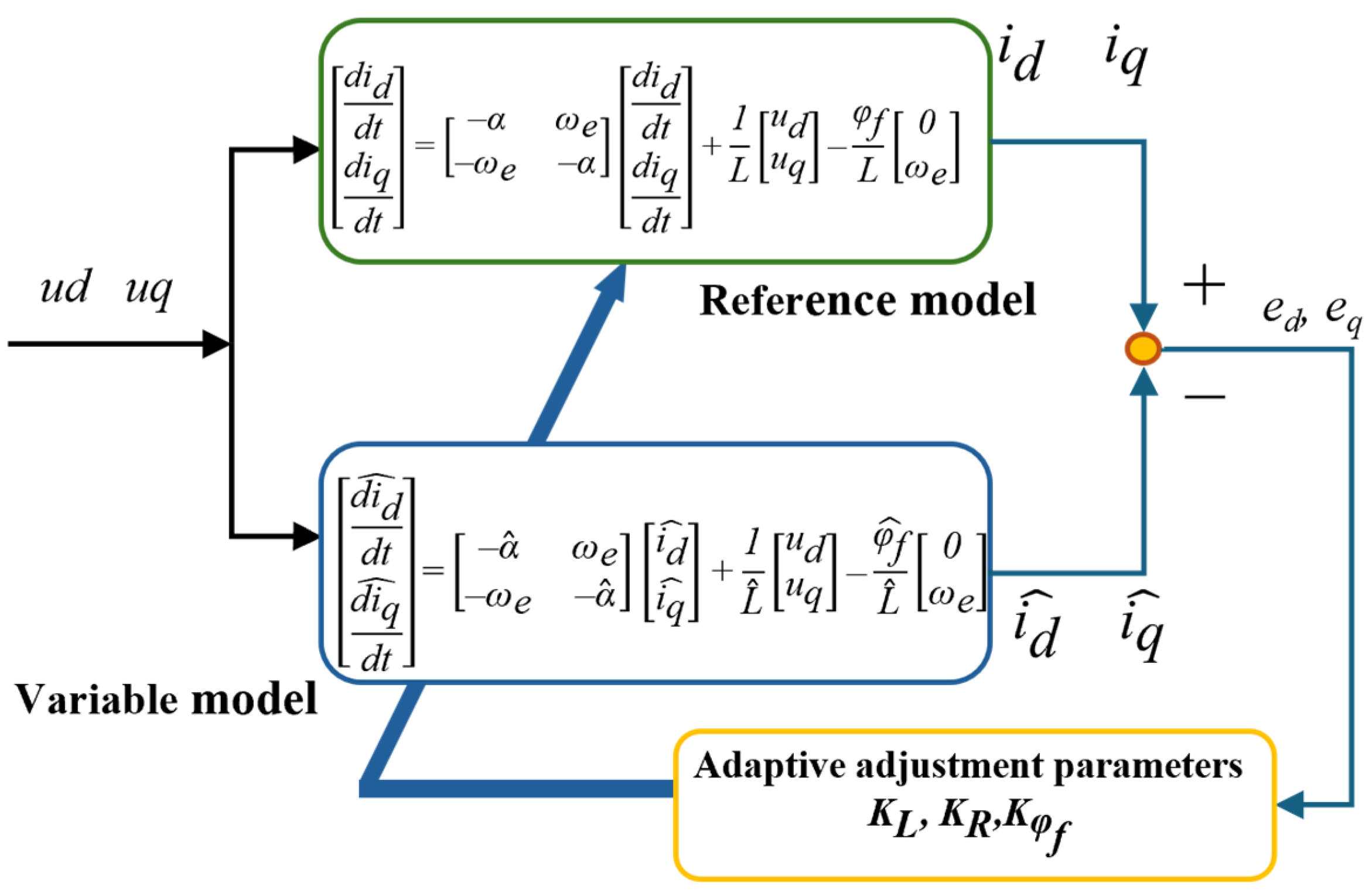
According to the MRAS, the parameter identification block diagram of the SPMSM based on the MRAS can be obtained as illustrated in Figure 1:

A summary of the specific steps to build the MRAS for the SPMSM can be derived from the block diagram:

• Choosing the dq-axis model of SPMSM as the reference model.
• Establishing a variable model of the SPMSM, where the parameters to be identified are adjustable variables and the inputs to the variable model are the same as those of the reference model.
• Obtaining the difference between the outputs of the reference model and the adjustable model; substitute the adaptive rules obtained from the above derivation and acquire the identification parameters from the regulation law.
• Substituting the identified parameters of the R, L, $\phi$ into the new variable model.

3. Moving Horizon Estimation

A.

General MHE Formulation

MHE is an optimized estimation method. It utilizes a limited amount of information regarding the input, output, and device models in order to identify the system state. The fundamental design of MHE is analogous to that of MPC, and thus it can also straightforwardly handle constraints and boundaries. However, in contrast to the prediction of future outcomes, MHE employs the output sliding window from the past. As a consequence of the significant advances in numerical optimization programs and the increased computing power of embedded control hardware, this field has attracted attention [28,29].

As illustrated in Figure 2, by introducing a fixed horizon of length N, the estimation problem at time k is divided into two parts: [0, …, k − N] and [k − N + 1, …, k]. The general state variable X_t is expressed in continuous real time. The black line represents the actual value of the state, red points represent the estimation result at time k, and blue points represent the estimation at time k + 1. In the process of estimation, the fixed window length N is maintained throughout. This guarantees that the length of the measurement information sequence required to estimate the state value at each moment remains unaltered. Consequently, the scale of optimization problem resolution in real time remains constant, and the other output information from the past is aggregated to the arrival cost. In the SPMSM model, the output current measurement data are represented by Equation (18):

$${\mathit{Y}}_{k-N}^{k-1}=\{{\mathit{y}}_{k-N},{\mathit{y}}_{k-N+1}, \dots ,{\mathit{y}}_{k-2},{\mathit{y}}_{k-1}\}$$

(18)

The superscript and subscript of the sequence symbol Y represent the start and end time of the measurement data sequence, respectively.

B.

Cost function and optimization of calculation.

Based on the nonlinear state space expression of disturbed SPMSM discretization described in Equation (6), the most recent N state values are presented in historical order.

$${\mathit{X}}_N=(\mathit{x}(k-N), \mathit{x}(k-N+1), \dots , \mathit{x}(k\left)\right)$$

(19)

It should be noted that when the estimated time of the initial stage is less than N, MHE will successfully resolve the full information estimation problem. The specific method has been provided by Rawlings et al. [13]. In this paper, we primarily discuss the case of estimation of times ≥ N. The constraints of SPMSM model, coupled with state and control inequality constraints, are considered. The minimized cost function is in (20) [14].

$$\min \mathit{J}\left({\mathit{X}}_N\right)={‖\mathit{x}(k-N)-\hat{\mathit{x}}(k-N)‖}_{{\mathit{P}}_{k-N}}^2+{\sum }_{i=k-N}^k{‖{\hat{\mathit{x}}}_{i+1}-f(\widehat{{\mathit{x}}_i},{\mathit{u}}_i)‖}_{{\mathit{Q}}^{-1}}^2$$

(20)

$$+{\sum }_{i=k-N}^k{‖{\mathit{y}}_i-\mathit{h}\widehat{{\mathit{x}}_i}‖}_{{\mathit{R}}^{-1}}^2 \mathrm{s}.\mathrm{t}.\left\{ \begin{array}{c}\mathit{x}\left(i\right)=f\left(\mathit{x}\right(i-1),\mathit{u}(i-1\left)\right)\hspace{1em}\hspace{1em}(\forall k-N⩽i⩽k)\\ \hspace{1em}\hspace{1em}\hspace{1em}\mathit{x}\left(i\right)\in \mathit{X}\hspace{1em}\hspace{1em}\hspace{1em}\hspace{1em}\hspace{1em} (\forall k-N⩽i⩽k)\\ \hspace{1em}\hspace{1em}\hspace{1em}\hspace{1em} \mathit{u}\left(i\right)\in \mathit{U}\hspace{1em}\hspace{1em}\hspace{1em}\hspace{1em}\hspace{1em} (\forall k-N+1⩽i⩽k)\end{array}\right.$$

${‖\mathit{x}(k-N)-\hat{\mathit{x}}(k-N)‖}_{{\mathit{P}}_{k-N}}^2$ represents the arrival cost of the MHE problem; P_k−N represents the posterior estimation covariance matrix of the k-N step state, which equals (21):

$${\mathit{P}}_{k-N+1}={\mathit{Q}}_{k-N}+{\mathit{F}}_{k-N}{\mathit{P}}_{k-N}{\mathit{F}}_{k-N}^T-{\mathit{F}}_{k-N}{\mathit{P}}_{k-N}{\mathit{h}}_{k-N}^T{({\mathit{R}}_{k-N}+{\mathit{h}}_{k-N}{\mathit{P}}_{k-N}{\mathit{h}}_{k-N}^T)}^{-1}{\mathit{h}}_{k-N}{\mathit{P}}_{k-N}{\mathit{F}}_{k-N}^T$$

(21)

The model Jacobian matrix is denoted as F_k and is defined as Equation (22):

$${\mathit{F}}_{\mathit{k}}={\frac{\mathbf{\partial }{\mathit{f}}^{\mathbf{2}}}{\mathbf{\partial }\mathit{x}}|}_{\mathit{x}=\widehat{{\mathit{x}}_{\mathit{k}}}}$$

(22)

In (22), x(i) represents the estimated state value at time i using MHE. $\hat{x}$(i) represents the predicted value at time i, which is calculated according to the system model using the instantaneous state estimation value at time i − 1 and the control input. X and U represent the state constraint set and input constraint set, respectively. Q_i and R_i are positive definite covariance matrices of w_k and v_k. The matrix Q represents the confidence level of the SPMSM model, while the matrix R represents the confidence level of the current measurement data.

Consequently, the state estimation problem is transformed into a fixed-horizon optimization problem by the MHE algorithm. This algorithm addresses system constraints, model interference, nonlinearity, and measurement noise. With the optimum solution ${\hat{\mathit{x}}}_{k-N}^{*}$, and iterating step by step according to the state equation of SPMSM, and iterating step by step according to the state equation of SPMSM, the state estimation of the current moment is calculated in Equation (23):

$$\begin{gathered} \mathit{x}(T-N+1)=\mathit{x}(T-N)+T_s[f\left(\mathit{x}\right(T-N\left)\right)+\mathit{gu}(T-N)+\mathit{w}(T-N\left)\right] \\ \mathit{x}(T-N+2)=\mathit{x}(T-N+1)+T_s\left[f\right(\mathit{x}(T-N+1\left)\right)+\mathit{gu}(T-N+1)+\mathit{w}(T-N+1\left)\right] \\ ⋮ \\ \mathit{x}\left(T) =\mathit{x}\right(T-1)+T_s\left[f\right(\mathit{x}(T-1\left)\right)+\mathit{gu}(T-1)+\mathit{w}(T-1\left)\right] \end{gathered}$$

(23)

The objective function in the optimization problem serves to define the moving horizon estimation method. Although this method is relatively straightforward and intuitive, it is challenging to implement and compute. In order to facilitate the computation of the MHE objective function optimization, the Hessian matrix and gradient vector are introduced to enhance the solving process [21].

At the k-Nth sampling time, the gradient vector of MHE has the following form:

$${\mathit{G}}_{E,k-N}=[\frac{\partial {\mathit{J}}_E}{\partial {\hat{\mathit{x}}}_{k-N}},\frac{\partial {\mathit{J}}_E}{\partial {\hat{\mathit{w}}}_{k-N}},\frac{\partial {\mathit{J}}_E}{\partial {\hat{\mathit{w}}}_{k-N+1}},\dots ,\frac{\partial {\mathit{J}}_E}{\partial {\hat{\mathit{w}}}_k}]$$

(24)

The elements that comprise the gradient vector are as follows:

$$\frac{\partial {\mathit{J}}_E}{\partial {\hat{\mathit{x}}}_{k-N}}=2{({\mathit{x}}_{k-N}-{\hat{\mathit{x}}}_{k-N})}^T{{\mathit{P}}_{k-N}\mathit{\Gamma }}_{k-N}+{\sum }_{i=k-N}^{k}2{\mathit{v}}_i^T{\mathit{Q}}_{k-N}\left(\frac{\partial {\mathit{v}}_i}{\partial {\hat{\mathit{x}}}_{k-N}}\right)$$

(25)

$$\frac{\partial {\mathit{J}}_E}{\partial {\hat{\mathit{w}}}_l}=2{\hat{\mathit{w}}}_l^T{\mathit{R}}_l{\mathit{\Gamma }}_{k-N}+{\sum }_{j=k-N}^k 2{\mathit{v}}_j^T{\mathit{Q}}_j\left(\frac{\partial {\mathit{v}}_j}{\partial {\hat{\mathit{w}}}_l}\right)$$

(26)

where ${\mathit{\Gamma }}_{k-N}$ is a vector with zero elements except the lth element.

Through the differential expression (23), the Hessian matrix H has the following symmetric form at the time of l sampling time:

$$\left[\begin{array}{ccc}\begin{array}{ccc}\frac{{\partial }^2{\mathit{J}}_E}{\partial {\hat{\mathit{x}}}_{k-N}\partial {\hat{\mathit{x}}}_{k-N}}& \frac{{\partial }^2{\mathit{J}}_E}{\partial {\hat{\mathit{x}}}_{k-N}\partial {\hat{\mathit{w}}}_{k-N}}& \frac{{\partial }^2{\mathit{J}}_E}{\partial {\hat{\mathit{x}}}_{k-N}\partial {\hat{\mathit{w}}}_{k-N+1}}\end{array}& \cdots & \frac{{\partial }^2{\mathit{J}}_E}{\partial {\hat{\mathit{x}}}_{k-N}\partial {\hat{\mathit{w}}}_k}\\ \begin{array}{ccc}\cdots & \frac{{\partial }^2{\mathit{J}}_E}{\partial {\hat{\mathit{w}}}_{k-N}\partial {\hat{\mathit{w}}}_{k-N}}& \frac{{\partial }^2{\mathit{J}}_E}{\partial {\hat{\mathit{w}}}_{k-N}\partial {\hat{\mathit{w}}}_{k-N+1}}\end{array}& \cdots & \frac{{\partial }^2{\mathit{J}}_E}{\partial {\hat{\mathit{w}}}_{k-N}\partial {\hat{\mathit{w}}}_k}\\ \begin{array}{ccc}\begin{array}{c}\cdots \\ \cdots \\ \cdots \end{array} & \begin{array}{c}\cdots \\ \cdots \\ \cdots \end{array}& \begin{array}{c}\frac{{\partial }^2{\mathit{J}}_E}{\partial {\hat{\mathit{w}}}_{k-N+2}\partial {\hat{\mathit{w}}}_{k-N+2}}\\ \cdots \\ \cdots \end{array}\end{array}& \begin{array}{c}\cdots \\ \cdots \\ \cdots \end{array}& \begin{array}{c}\frac{{\partial }^2{\mathit{J}}_E}{\partial {\hat{\mathit{w}}}_{k-N+2}\partial {\hat{\mathit{w}}}_k}\\ \cdots \\ \frac{{\partial }^2{\mathit{J}}_E}{\partial {\hat{\mathit{w}}}_k\partial {\hat{\mathit{w}}}_k}\end{array}\end{array}\right]$$

(27)

The Hessian matrix elements are given by (28)–(30)

$$\begin{gathered} \frac{{\partial }^2{\mathit{J}}_E}{\partial {\hat{\mathit{x}}}_{k-N}\partial {\hat{\mathit{x}}}_{k-N}}=2{\mathit{\Gamma }}_{k-N}^T{\mathit{P}}_{k-N}{\mathit{\Gamma }}_{k-N}+2{\sum }_{i=k-N}^k{\left(\frac{\partial {\mathit{v}}_i}{\partial {\hat{\mathit{x}}}_{k-N}}\right)}^T{\mathit{Q}}_{k-N}\left(\frac{\partial {\mathit{v}}_i}{\partial {\hat{\mathit{x}}}_{k-N}}\right) \\ +2{\sum }_{i=1}^N{\mathit{v}}_i^T{\mathit{Q}}_{k-N}\left(\frac{{\partial }^2{\mathit{v}}_i}{\partial {\hat{\mathit{x}}}_{k-N}\partial {\hat{\mathit{x}}}_{k-N}}\right) \end{gathered}$$

(28)

$$\frac{{\partial }^2{\mathit{J}}_E}{\partial {\hat{\mathit{x}}}_{k-N}\partial {\hat{\mathit{w}}}_{\alpha }}=2{\sum }_{i=k-N}^k{\left(\frac{\partial {\mathit{v}}_i}{\partial {\hat{\mathit{x}}}_{k-N}}\right)}^T{\mathit{Q}}_{k-N}\left(\frac{\partial {\mathit{v}}_i}{\partial {\hat{\mathit{w}}}_{\alpha }}\right)+2{\sum }_{i=k-N}^k{\mathit{v}}_i^T{\mathit{Q}}_{k-N}\left(\frac{{\partial }^2{\mathit{v}}_i}{\partial {\hat{\mathit{x}}}_{k-N}\partial {\hat{\mathit{w}}}_{\alpha }}\right)$$

(29)

$$\begin{gathered} \frac{{\partial }^2{\mathit{J}}_E}{\partial {\hat{\mathit{w}}}_{\alpha }\partial {\hat{\mathit{w}}}_{\beta }}=2{\mathit{\Gamma }}_{\alpha }^T{\mathit{R}}_{k-N}{\mathit{\Gamma }}_{\beta }^T+2{\sum }_{i=k-N}^k{\left(\frac{\partial {\mathit{v}}_i}{\partial {\hat{\mathit{w}}}_{\alpha }}\right)}^T{\mathit{Q}}_{k-N}\left(\frac{\partial {\mathit{v}}_i}{\partial {\hat{\mathit{w}}}_{p,k}}\right) \\ +2{\sum }_{i=k-N}^k{\mathit{v}}_i^T{\mathit{Q}}_{k-N}\left(\frac{{\partial }^2{\mathit{v}}_i}{\partial {\hat{\mathit{w}}}_{\alpha }\partial {\hat{\mathit{w}}}_{\beta }}\right) \end{gathered}$$

(30)

Furthermore, when the state is updated, the state at time k can be updated by the Carleman approximate Formula (31) [30].

$${\hat{\mathit{x}}}_k={\mathit{A}}^N{\hat{\mathit{x}}}_{k-N}^{*}+{\sum }_{i=0}^{N-1}{\mathit{A}}^i\left(\mathit{g}{\mathit{u}}_{k-i}+{\hat{\mathit{w}}}_{k-i}\right)$$

(31)

The state of k–N+1 moment is updated by (32)

$${\hat{\mathit{x}}}_{k-N+1}={\mathit{A}}_{k-N}{\mathit{P}}_{k-N}{\mathit{h}}^T{\left(\mathit{h}{\mathit{P}}_{k-N}{\mathit{h}}^T+\mathit{R}\right)}^{-1}\left({\mathit{y}}_{k-N}-\mathit{h}{\hat{\mathit{x}}}_{k-N}^{*}\right)+{\mathit{A}}_{k-N}{\hat{\mathit{x}}}_{k-N}^{*}$$

(32)

where ${\mathbf{A}}_{k-N}={\left.\frac{\partial f_{k-N}(\mathit{x},0)}{\partial \mathit{x}}\right|}_{{\hat{\mathit{x}}}_{k-N}^{*}}$,${\hat{\mathit{x}}}_{k-N}^{*}$ is the optimal solution of MHE.

C.

SPMSM sensorless controller strategy

The MHE-based sensorless observation strategy comprises the following steps:

(I).

Initialization: setting covariance matrices Q, P, R, the initial state x (0) = [0 0 0]^T, and the moving horizon window size N.

(II).

Let the current time be k, and when k ≤ N, the problem of full information estimation is solved, and the state estimation value of the current time is calculated by Equation (31).

(III).

When k ≥ N, the gradient vector (24) and the Hessian matrix (27) are employed to solve function (20) in order to obtain the optimal solution, and the current state estimate is calculated using Equation (31).

(IV).

The error covariance matrix P_k−N and the prior estimated state of the next moment $\hat{x}(k-N)$ are calculated according to Equations (21) and (32).

(V).

Adding a new output data y_T and reconstructing the output sequence, returning (II).

The sensorless control scheme of the SPMSM is depicted in Figure 3. The system employs current loop and rotational speed loop control for the current inner loop and speed exchange. The principal components of the system include a control module, MHE observer module, MRAS parameter identification module, Clarke conversion and Park conversion module, inverter, and SVPWM module.

Through the detection of the current by the MHE observer, the rotational speed and electrical angle of the motor are calculated. Concurrently, the acquired stator three-phase current is transformed into the dq coordinate system through Clark and Park transformations. Through the speed adjustment module, the reference value of the Q-axis current is obtained. Subsequently, the stator current fed back by the dq-axis is then compared to the reference dq-axis current, and the dq-axis voltage is obtained by the current regulator.

With the combination of voltage and current, two models and a parameter adaptive law are designed using MRAS. Firstly, two independent structures, the reference model and the adjustable model, are constructed in accordance with the mathematical equation of the motor. The adjustable model is constructed based on the parameters to be identified, while the reference model is derived from the fundamental voltage and current equations. The inputs of the two models are aligned, thereby enabling the real-time determination of motor parameters such as resistance, inductance, and flux.

In most cases, the SPMSM uses a DC source for its power supply. Consequently, it is of paramount importance to utilize the inverter circuit in order to achieve the AC-DC conversion of the drive circuit. This entails using the SVPWM modulation technology to control the inverter’s switching through six-channel PWM signals. This process enables the inversion of DC into sinusoidal AC, which serves a significant purpose. The main circuit module relies on the vector control SVPWM module to supply the necessary signal. This generates the PWM signal, which regulates the inverter’s switching and ultimately outputs the operation of the three-phase AC drive motor. The inverter employs a three-phase IGBT inverter bridge, in which a DC voltage source powers supplies the DC terminal, while an AC terminal generates three-phase AC voltage to drive the SPMSM.

4. Simulation Results

A.

Set up Description.

The sensorless controller of the PMSM has been implemented in MATLAB 2020b. The sampling time of the simulation is 1 × 10⁻⁴ s. In the observer, a Gaussian noise with a μ of 0 and a σ of 0.2 is applied to i_d and i_q. The parameters are set as in

Table 1. Parameters.

Number of poles/Pn	4
Stator resistance/RS	2.7 Ω
Synchronous inductance/LS	8 mH
$\mathrm{Flux} \mathrm{linkage}/{\phi }_f$	0.17 WB
Motor inertia/J	0.003 Kgm2
Coefficient of viscous friction/Bm	0.01
$\mathrm{Rated} \mathrm{speed}/\omega$	1200 rpm
Horizon/N	5
Process noise covariance matrix/Q	diag([0.1 0.1 1])
Measurement noise covariance matrix/R	diag([0.2 0.2])
State covariance matrix/P	diag([0.1 0.1 0])

:

This chapter primarily examines the performance of speed and rotor position observation in the SPMSM. To eliminate any ambiguity in the results of the simulation, two separate simulation scenarios were chosen. In each scenario, we allocated different values for the rated reference speeds and reference torques. MHE is primarily evaluated against conventional observers, such as EKF and SMO, in order to assess the effectiveness of MHE. The system’s dynamic features, accuracy, and parameter sensitivity are investigated by simulation. Furthermore, this study also examines the impact of varying estimated horizon N on the observation effect of MHE, the enhancement of estimation accuracy following the inclusion of MRAS, and the optimization effect of the Hessian matrix and gradient vector on the computational workload. The evaluation of speed and angle estimate performance employs two criteria: the root mean square error (RMSE) and absolute error (AE), which are described as follows:

$$\begin{array}{c}\mathrm{R}\mathrm{M}\mathrm{S}\mathrm{E}=\sqrt{\frac{{\sum }_{i=1}^k{|{\hat{\omega }}_{\mathit{ri}}-{\omega }_{\mathit{ri}}|}^2}{k}}\\ {\mathrm{AE}}_i=|{\hat{\omega }}_{\mathit{ri}}-{\omega }_{\mathit{ri}}|\end{array}$$

B.

Simulation results under Condition I

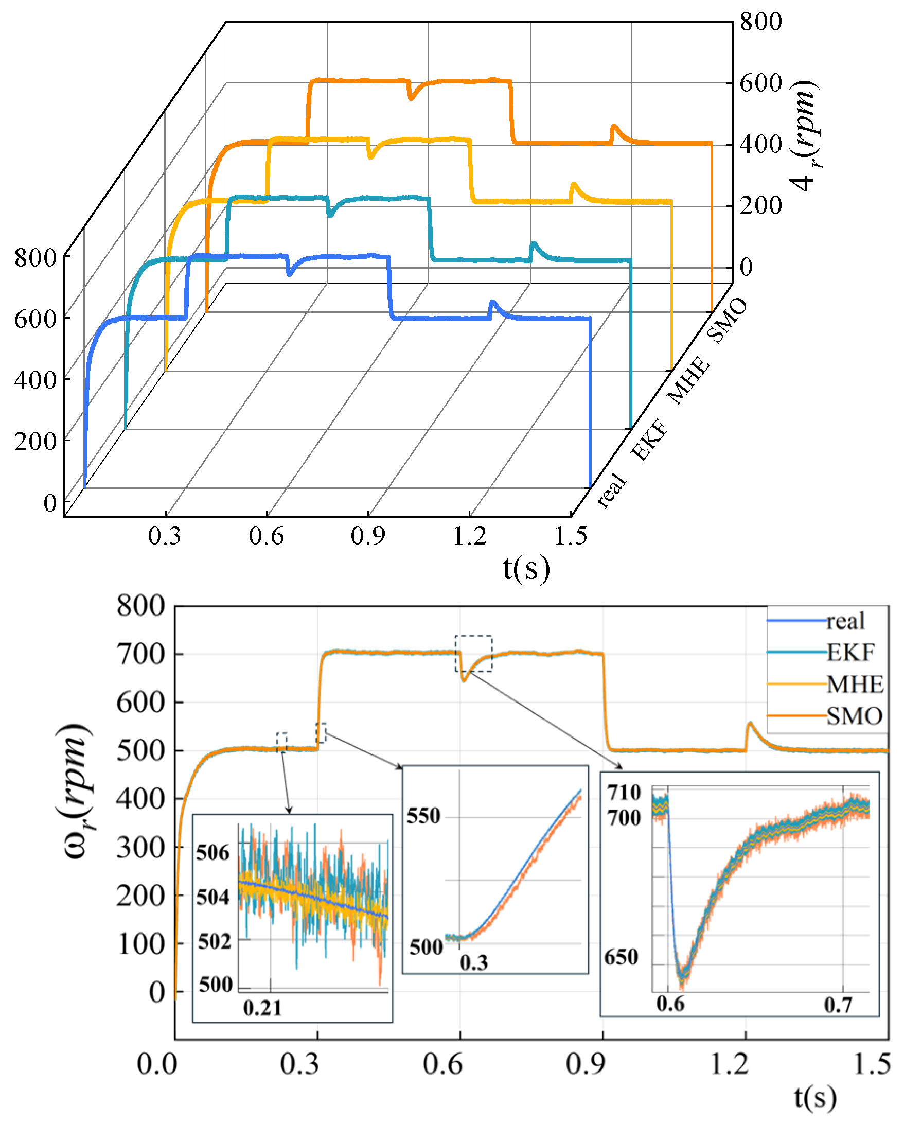
Under Condition I, the initial settings are as follows: The initial reference speed ω_ref is set as 500 rpm, while the reference load torque is set as 20 Nm. At a time of 0.3 s, the reference speed reaches 700 rpm. At a time of 0.6 s, the reference load torque increases to 30 Nm. At a time of 0.9 s, the reference speed returns to 500 rpm, and at a time of 1.2 s, the reference load torque returns to 20 Nm. A dual PI controller is employed in both the speed loop and current loop.

Figure 4 displays the outcomes of estimating the rotational speed of the SPMSM using three distinct witnesses. Figure 5 presents the measurement of i_d and i_q, while Figure 6 illustrates the inaccuracy in the estimation for each of the three observers. During the initial phase of increased activity, the SMO estimator experiences fluctuations in performance, resulting in a maximum estimation error of approximately 10 rpm. The estimation of MHE exhibits significant variability during the initial stage, but as the system undergoes dynamic changes, it eventually stabilizes and reaches a steady state within the first 30 ms.

Upon reaching a reference speed of 500 rpm and stabilizing, it can be observed that MHE exhibits superior tracking performance in comparison to EKF and SMO, with an estimation error of less than 2 rpm. When the reference speed changes quickly, at 0.3 s, the capacity of SMO to track the rotational speed is significantly diminished, with an error rate of up to 10.9 rpm. Following a tuning process of 10 ms, the system finally converges, but its dynamic performance is slower than that of EKF and MHE. Following the abrupt alteration in load torque at 0.6 s, the EKF exhibits an average estimation error of 0.71 rpm, which converges by approximately 0.2 rpm. Concurrently, the SMO continues to exhibit an error of approximately 1.2 rpm. The MHE exhibited optimal dynamic response throughout the sudden speed change of 0.9 s, with an average speed estimation error of 0.9 rpm throughout the dynamic response time. The dynamic response times of the three estimators are comparable. However, SMO exhibited a larger overshoot. In general, by effectively utilizing the historical data within the horizon window, the MHE observer demonstrates impeccable accuracy in estimating both transient and steady-state processes. In addition to maintaining excellent dynamic performance, the mean estimation error of the MHE is merely 0.279 rpm, which is approximately 35.7% of the EKF and 21.4% of the SMO.

Table 2. Quantitative measurement of the inaccuracy in speed estimation, under condition I.

	Maximum	Minimum	Average	RMSE
SMO	57.034	5.155 × 10−7	1.302	2.213
EKF	4.936	1.434 × 10−6	0.782	0.975
MHE	2.531	3.628 × 10−8	0.279	0.360

presents the specific speed error.

Figure 7 and Figure 8 depict the monitoring of the rotor’s position by three distinct observers. The maximal estimation error of SMO is 1.5 rad, and that of MHE is only 0.5 rad.

Table 3. Quantitative measurement of the inaccuracy in position estimation, under condition I.

	Maximum	Minimum	Average	RMSE
SMO	1.689	6.657 × 10−6	0.406	0.629
EKF	1.631	2.358 × 10−7	0.806	0.934
MHE	0.744	5.986 × 10−6	0.347	0.432

demonstrates that the MHE method provides a more precise estimation of the rotor position.

C.

Simulation results under Condition II

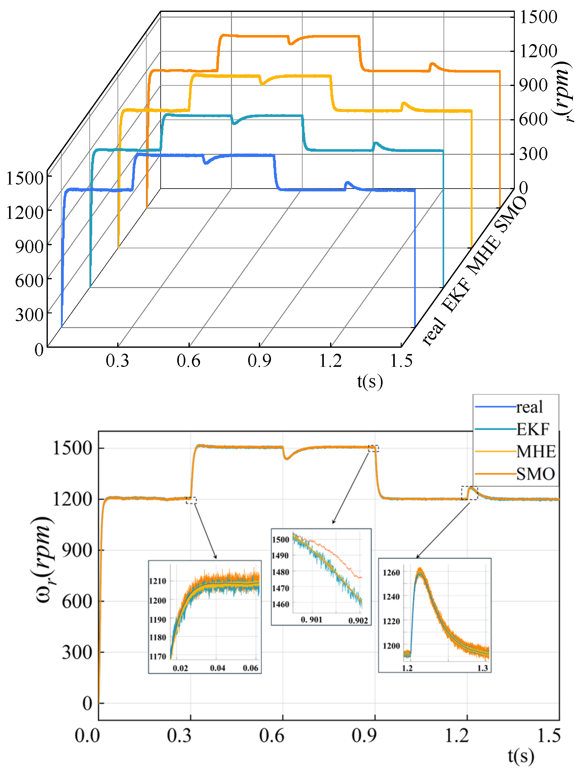
Under Condition II, the initial reference speed ω_ref is set at 1200 rpm, while the reference load torque is set at 5 Nm. At 0.3 s, the reference speed changes to 1500 rpm, and the reference torque of 10 Nm is applied at 0.6 s. The reference speed returns to its rated value of 1200 rpm at 0.9 s, and the reference torque decreases to 5 Nm at 1.2 s.

Figure 9 and Figure 10 depict the recorded speed, whereas Figure 11 illustrates the measurement of i_d and i_q.

Table 4. Quantitative measurement of the inaccuracy in speed estimation, under Condition II.

	Maximum	Minimum	Average	RMSE
SMO	32.276	4.317 × 10−7	1.329	2.290
EKF	9.071	1.534 × 10−6	1.328	1.706
MHE	7.144	1.362 × 10−6	0.425	0.634

demonstrates that the estimation error of SMO and EKF has decreased by 10% in comparison to Condition I. Nevertheless, the MHE maintains both satisfactory estimation accuracy and a rapid dynamic reaction time, despite initially displaying a maximum tracking error of −7 rpm, it rapidly converges within 10 ms, with the greatest error amounting to 21.7% of the SMO. While the reaction time of the EKF is comparable to that of the MHE, the average estimation error of the EKF is approximately 1.3 rpm, which is 2.8 times higher than that of the MHE. Although the average steady-state estimation error of SMO is less than that of EKF, it is important to note that SMO has a longer response time in the event of a sudden change in reference load torque. Furthermore, when SMO is employed, the estimation error increases during dynamic perturbations, indicating that SMO has weaker robustness compared to EKF and MHE.

Figure 12 and Figure 13 present the recorded measurements of rotor position as observed by three distinct individuals. The estimation error of MHE is observed to be within a range of ±0.5 rad and exhibits a progressive convergence as time progresses. As indicated in

Table 5. Quantitative measurement of the inaccuracy in position estimation.

	Maximum	Minimum	Average	RMSE
SMO	1.401	2.667 × 10−7	0.759	0.839
EKF	1.37	9.572 × 10−10	0.570	0.632
MHE	0.414	2.668 × 10−10	0.362	0.357

, the RMSE of MHE method is 46.5% more convergent than that of EKF and 59.2% more convergent than that of SMO.

The experimental results demonstrate that when a disturbance occurs in the control system, this results in a significant increase in the tracking delay in the SMO. Under Condition I, EKF is more effective in speed estimation, although the tracking sensitivity decreases slightly under Condition II. Both experimental conditions demonstrate the robustness of MHE, with its estimation errors being smaller than those of EKF and SMO.

D.

The impact of varying horizon N on the precision of estimation

It can be demonstrated that alterations in the horizon will lead to modifications in the outcomes of MHE estimation. An increase in the horizon will enhance the precision of the estimation, yet it will also result in a slower response time due to the necessity to process a greater quantity of data. Conversely, reducing the horizon will expedite the calculation but will also result in a reduction in the accuracy of the estimate. In order to enhance the efficiency of comprehensive estimation and to explore the optimal horizon of MHE, experiments were conducted under condition II using N = 3, 5, 10.

Figure 14, Figure 15 and Figure 16 illustrates that the estimation accuracy of MHE(N = 5) exceeds that of N = 3 as a consequence of the utilization of a greater quantity of historical data, which results in a more precise noise probability distribution density. In this scenario, the efficiency of MHE improves as the length of the horizon increases.

Nevertheless, when the value of N is set to 10, the improvement in estimating accuracy will not be significant despite the expansion of the horizon. This finding aligns with prior study conducted by Rao et al. [29]. The optimal value for the horizon is equal to twice the order of the system, resulting in a reduced computing load while maintaining estimation accuracy.

E.

The impact of MRAS on the estimation outcome

MRAS has been the primary subject of research in the field of servo industrial systems. The design of the MHE observer is inextricably linked to the internal parameters of the SPMSM. During the operation of the SPMSM, the internal parameters undergo changes. If the MHE continues to utilize the parameters established at the step of initialization, it will inevitably result in a decline in estimation accuracy.

This section presents a comparison between the MHE with MRAS and the ordinary estimator. The experiments are conducted under Condition II. During the operation of the SPMSM, the values of R, L, and φ are subject to change. The adaptive rate setting for the MRAS is displayed in

Table 6. Value of MRAS adaptive rate.

Adaptive rate of inductance model/KL	300
Adaptive rate of stator resistance model/KR	300
Adaptive rate of flux model/Kφ	100

.

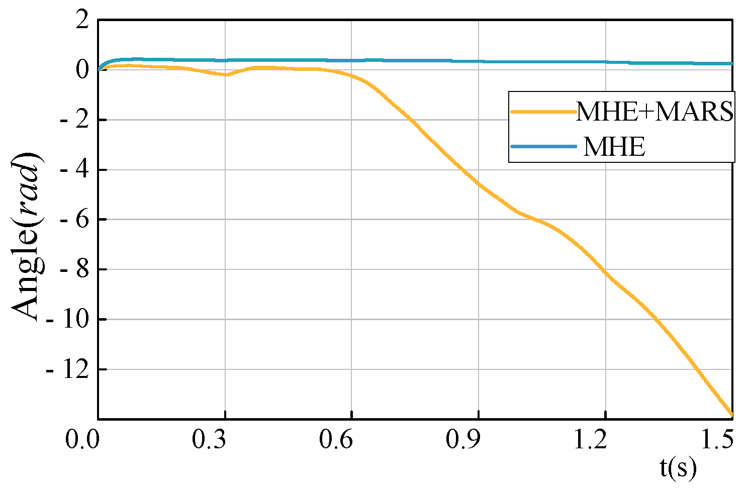
Figure 17 and Figure 18 illustrate the outcomes of speed and rotor position estimation using MHE with MRAS parameter identification in comparison to the conventional MHE. Figure 19 presents the RMSE values for two distinct techniques. The RMSE of the estimation error in MHE without parameter identification is approximately 12.3 times higher than that of MHE utilizing MRAS. Furthermore, the error of position estimation is also approximately 17 times higher. Consequently, in real-world scenarios, the parameter identification of the SPMSM control system is of paramount importance to the observer, since the precision of parameter estimation directly impacts the control accuracy. Figure 20 illustrates the projected outcomes of the SPMSM’s characteristics as estimated using the MRAS.

F.

Optimization of computation

Figure 21 and Figure 22 illustrate the speed and rotor position estimation achieved by the general MHE and optimized MHE methods, respectively, utilizing the Hessian matrix and gradient vector. The estimation error and computation time are presented in

Table 7. Estimation error and computation time.

	∆ωr AVE	∆ωr RMSE	∆Angle AVE	∆Angle RMSE	Compute Time
Optimized MHE	0.626	0.891	0.406	0.412	70.436 s
Normal MHE	0.475	0.692	0.334	0.338	181.128 s

. By utilizing the Hessian inverse matrix as the search length for optimization, the step size is adjusted in each iteration, thereby reducing the average estimation error of speed and rotor position to below 20% when compared to the original technique. By retaining the accuracy of the estimation, the computation time has been reduced from 181.13 s to 70.44 s, resulting in a 61.13% decrease in the quantity of calculation. The optimization of computation offers significant advantages in practice, allowing the processor to reduce memory usage and effectively satisfy the demands of the SPMSM fast control system.

5. Conclusions

This study has successfully demonstrated the sensorless drive of the SPMSM. A nonlinear model of the system has been constructed, taking into account the varying parameters of stator inductance, stator resistance, and flux of SPMSM during actual operation. In order to ascertain the motor’s parameters in real time, the MRAS is employed. A methodology for estimating the speed and rotor position of a SPMSM without using sensors is suggested. MHE, which is an optimization-based approach, achieves exceptional accuracy. The EQP optimization problem is efficiently solved in real time by utilizing the gradient vector and Hessian matrix, which incur minimal computing costs in each iteration.

A comprehensive analysis has been proposed to assess the performance of the MHE scheme and to compare it to the established approaches, specifically EKF and SMO. The experimental findings demonstrate that the control framework proposed in this research study exhibits superior robustness and can serve as a comprehensive solution for sensorless control of SPMSM.

In the current hardware control system for PMSM, the sensorless control scheme is primarily employed to accomplish the control task at a frequency of 10 kHz. This is achieved by detecting the current and voltage in the d-axis and q-axis and generating three-phase PWM signals using the suggested observer and controller at each sampling interval. This control scheme does not necessitate the use of an optical encoder and is compatible with 32-bit MCUs and FPGAs. One potential issue that may arise is the risk of insufficient computational memory while the MCU is engaged in multitasking. It is conceivable that in the future, the MHE optimization problem could be streamlined by employing data-driven or neural network algorithms without compromising the resilience of the PMSM control system.