Abstract
Unmanned aerial vehicle (UAV) navigation plays a crucial role in its ability to perform autonomous missions in complex environments. Most of the existing reinforcement learning methods to solve the UAV navigation problem fix the flight altitude and velocity, which largely reduces the difficulty of the algorithm. But the methods without adaptive control are not suitable in low-altitude environments with complex situations, generally suffering from weak obstacle avoidance. Some UAV navigation studies with adaptive flight only have weak obstacle avoidance capabilities. To address the problem of UAV navigation in low-altitude environments, we construct autonomous UAV navigation in 3D environments with adaptive control as a Markov decision process and propose a deep reinforcement learning algorithm. To solve the problem of weak obstacle avoidance, we creatively propose the guide attention method to make a UAV’s decision focus shift between the navigation task and obstacle avoidance task according to changes in the obstacle. We raise a novel velocity-constrained loss function and add it to the original actor loss to improve the UAV’s velocity control capability. Simulation experiment results demonstrate that our algorithm outperforms some of the state-of-the-art deep reinforcement learning algorithms performing UAV navigation tasks in a 3D environment and has outstanding performance in algorithm effectiveness, with the average reward increasing by 9.35, the success rate of navigation tasks increasing by 14%, and the collision rate decreasing by 14%.
1. Introduction
In recent years, unmanned aerial vehicles (UAVs) have been widely used in military and civilian fields, such as material delivery [1,2], aerial photography [3], and emergency rescue [4] due to their low manufacturing cost and high flexibility. The basis for UAVs to perform these tasks is their ability to fly to their destination safely and autonomously in complex environments [5].
Many researchers have used traditional path planning algorithms (e.g., A* [6], RRT [7], and artificial potential field [8] algorithms) as well as intelligent optimization algorithms (e.g., particle swarm optimization [9,10], ant colony optimization [11], and genetic algorithms [12]) to achieve autonomous UAV navigation. However, these non-learning algorithms require global information and perfect action execution mechanisms to plan feasible paths in a given environment [13,14,15,16,17]. It is difficult for them to handle unknown environments, and there are disadvantages such as poor real-time performance, weak online navigation, and obstacle avoidance capabilities.
Given the sequential decision-making characteristics of UAV navigation, many researchers model the problem as a Markov decision process (MDP) and study it using deep reinforcement learning [18]. Reinforcement learning makes decisions guided by a reward function and does not require global information. It enables a UAV to perform navigation and obstacle avoidance tasks autonomously under various constraints.
Many existing studies have introduced memory to improve autonomous UAV navigation ability in complex environments. Wang et al. [19] constructed UAV navigation as a partially observable Markov decision process (POMDP) and used historical trajectories as input to train the action policy of the UAV. They demonstrated that in the POMDP problem, the network could be trained not only using the complete trajectory data of an episode but also using the historical trajectories of each step. With this theory as the cornerstone, they proposed the Fast-RDPG algorithm based on the RDPG algorithm [20], which improves the utilization of sample data and the convergence speed of the model. Fu et al. [21] used images taken by an airborne monocular camera as input and constructed UAV navigation as an MDP for target conditions. They improved the DQN algorithm [22] by using the absolute coordinates of the target point instead of its relative coordinates with respect to the position of the UAV. A merging of spatial memory and action memory was proposed in their work to process the historical trajectories of the UAV, and an attention module was used to improve the perception of the algorithm. Singla et al. [23] also used image data as input to the reinforcement learning model. They first transformed the RGB three-channel pictures into depth pictures to facilitate the extraction of distance information. Then, they added the CNN, LSTM (Long Short-Term Memory), and attention to the DQN model to achieve UAV obstacle avoidance flight in an indoor environment. Several of the above studies were conducted in the environment of fixed UAV flight altitude and flight velocity. After extending their model into an adaptive control (The UAV will learn to control the flight altitude and flight speed by itself), the convergence speed and obstacle avoidance ability of the model were greatly reduced. And in a low-altitude, multi-obstacle environment, the experimental results of their model do not work well.
To solve the problem of difficulty in obstacle avoidance of UAVs with adaptive control, Zhang et al. [24] proposed a kind of two-stream structure. When making action decisions and state evaluations, they used not only the current state but also input the state vector difference between the current time step and the previous time step, which is used to represent the change in the state and improve the algorithm’s perception of the changing environment. The state vector is normalized to improve the feature extraction ability and the convergence speed of the algorithm. But they did not consider improvements at the decision level; the performance of the method may not be good in more complex environments. Our reproduction experiments performed in 3D complex environments prove this. Based on an AC framework, Guo et al. [25] divided the actor network into “acquire”, “avoid”, and “pack” networks separately to address the navigation task and the obstacle avoidance tasks and select whether to execute a navigation or obstacle avoidance policy. With the dynamically changing flight trajectories as the input data, they used DQN and LSTM to address the UAV navigation and obstacle avoidance problem in a moving obstacle environment. However, while this method enhances a UAV’s obstacle avoidance capability, it also fragments the entire decision-making part, making it difficult to combine navigation and obstacle avoidance. Although both of the above methods improve the obstacle avoidance ability of the UAV, their models’ performance is lower under the condition of adaptive control in low-altitude environments with complex situations. Hu et al. [26] proposed a deep reinforcement learning algorithm based on Proximal Policy Optimization (PPO) to lead UAVs to their destinations through continuous control. A kind of scenario state representation and corresponding reward function were raised to map the observation space to both heading angle and speed. Their algorithm has achieved good results in a 2D environment with few obstacles and simple features, but if migrated to a complex 3D environment, the efficiency of the algorithm will decrease.
Several studies have optimized the experience replay buffer in deep reinforcement learning. Schaul et al. [27] propose a Prioritized Experience Replay (PER) sampling method. They sort the samples in the empirical replay buffer pool in the order of TD-error from smallest to largest and prioritize the samples with TD-error for learning to enhance the convergence speed of the algorithm. Hu et al. [28] designed a sampling method with double-screening, implementing it based on the Deep Deterministic Policy Gradient (DDPG) algorithm, and proposed the Relevant Experience Learning-DDPG (REL-DDPG). They used a Prioritized Experience Replay (PER) mechanism to imitate human learning by finding the most similar experience to the current observation for training to enhance the learning ability and convergence speed of the UAV model. This is an optimization method from the perspective of training samples and does not involve the optimization of strategies. This model can only learn the samples generated by the original navigation and obstacle avoidance strategy, which has a limited effect on the improvement in obstacle avoidance capability.
In addition, there is research using imitation learning to solve the problem of autonomous UAV navigation. Loquercio et al. [29] used expert data and data collected from car driving and bicycle riding as demonstrations to train residual neural networks and conduct UAV navigation experiments in an urban, high-altitude environment that contains sparse dynamic obstacles. Following the literature [19], Wang et al. [30] considered that most decision processes lacked reward signals, further exploring the UAV navigation problem in a sparse reward case. For the first time, they constructed UAV navigation in complex environments as a sparsely rewarded MDP problem and proposed the LwH algorithm based on imitation learning. This algorithm uses a priori policies and learns new policies to jointly determine the behavior of the UAV, using nonexpert helper policies to help the UAV explore space and learn. However, the LwH algorithm requires accurate, large, and diverse expert demonstrations to guide the UAV in their navigation missions, which is more difficult to achieve because of the high data quality requirements.
The above research shows that deep reinforcement learning has made many achievements in the field of autonomous UAV navigation, but there are still problems. Some studies have fixed the flight speed and altitude of UAVs, making them unsuitable for navigating in complex, low-altitude environments. Some studies have provided adaptive flight control for UAVs, but their algorithms have weak obstacle avoidance ability in complex low-altitude environments. To improve the obstacle avoidance capability of UAVs under adaptive control, the guide attention recurrent TD3 (GARTD3) algorithm with a novel velocity-constrained loss function is proposed in this paper. The main contributions of this paper are as follows:
- To solve the problem of difficult obstacle avoidance brought by adaptive control, we creatively propose to guide attention to make the decision center of the UAV shift between the navigation task and the obstacle avoidance task according to the environment;
- To help the UAV learn speed control, we present a novel velocity-constrained loss function with a regulating factor, further improving the UAV’s obstacle avoidance capability. Motivated by (1) and (2), a learning algorithm is proposed based on the TD3, LSTM, and attention;
- A complex 3D simulation environment for UAV navigation is established, and experiment results prove that our method can improve the autonomous navigation and obstacle avoidance capability of the UAV, outperforming some of the state-of-the-art reinforcement learning algorithms in the UAV navigation field.
The remainder of this paper is outlined as follows: Section 2 introduces the modeling approach with adaptive control in detail. In Section 3, the basic algorithm, the core innovations we propose, and the overall algorithm are presented. In Section 4, simulation results are presented to verify the effectiveness of our algorithm. Finally, Section 5 concludes the work and discusses the future prospects of this research.
2. Problem Formulation and POMDP Molding
2.1. Problem Formulation
Quadrotor UAVs are widely used in various research because of their high flexibility, easy maneuverability, and applicability to various environments. In this paper, we also use the quadrotor UAV as a research subject to study the UAV navigation problem under adaptive flight and control the UAVs from the perspective of kinematics.
UAVs use onboard sensors to sense the external environment when performing navigation tasks in a 3D environment. However, using observations from only one step does not provide a description of the entire environment; UAVs in complex environments need to introduce historical trajectories to sense the external environment, which is also helpful to make decisions.
Therefore, in this study, the UAV navigation problem in 3D complex environments is constructed as a POMDP, which can be represented by a seven-tuple . denotes the state space, which is a hidden variable and is not defined explicitly in the POMDP; is the action space; is the state transfer probability; is the reward function, determined by the current state and action; is the observation probability; is the observation space, and is the discount factor. In the POMDP model, the observation space and action space could be continuous or discrete, corresponding to the action decision functions and , respectively. For the UAV autonomous navigation task, the control signals are continuous in the real environment, so we will use the continuous action space to control the flight of the UAVs.
2.2. POMDP Modeling of UAV Navigation with Adaptive Control
In the POMDP model, state transfer probability and the discount factor are defined by the algorithm, and the observation probability is defined by the environment. Therefore, in this subsection, the POMDP modeling process for UAV navigation in a 3D environment is described in terms of the observation space , action space , and reward function . When constructing the POMDP model, we refer to the MDP modeling work of the literature [23,24,25,30], add new environmental data to enhance the perceptual capabilities of the model and use an action space that satisfies adaptive control conditions.
The overall observation space is designed as
where , and represent the coordinates of the target point with respect to the current position of the UAV in the global coordinate system.
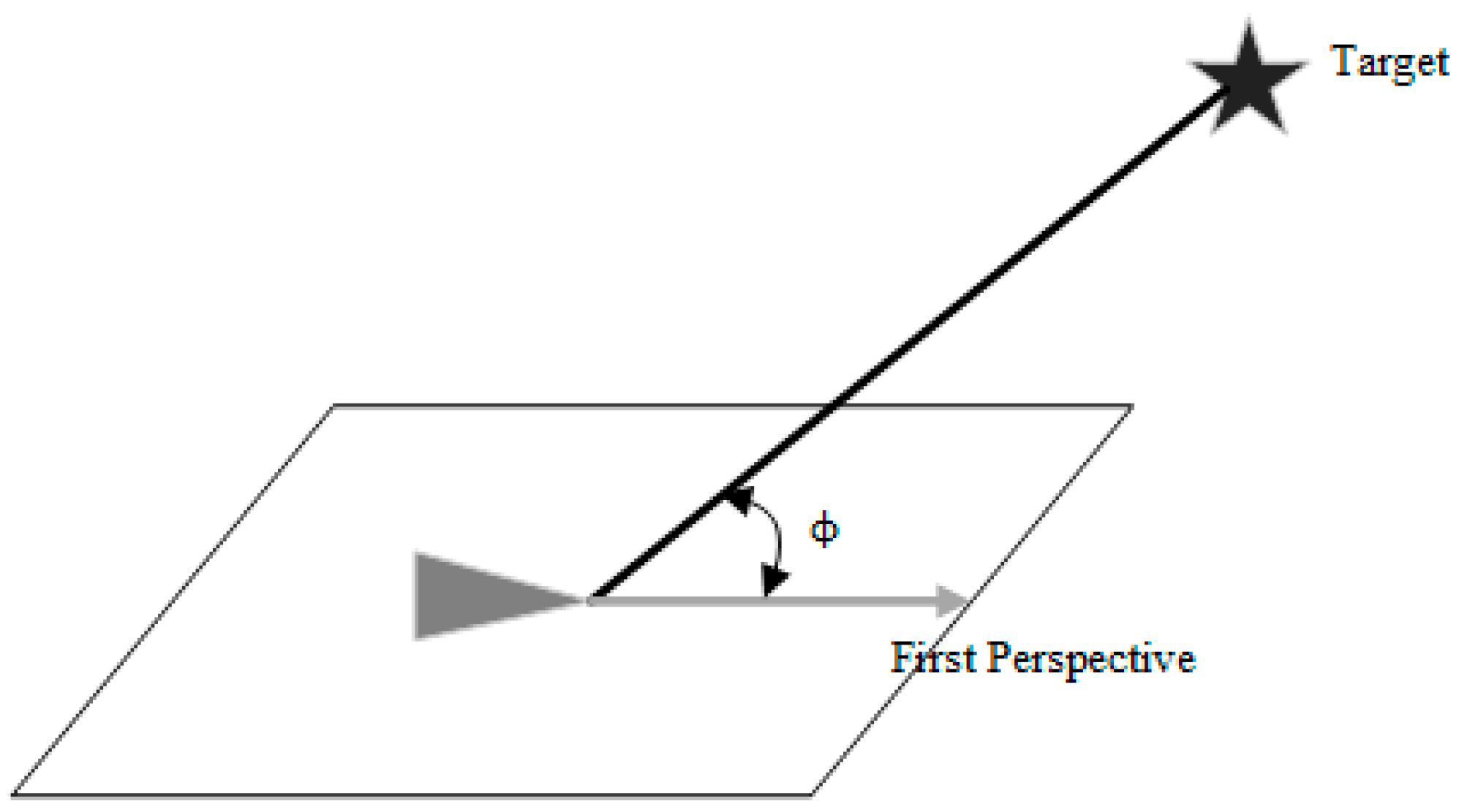
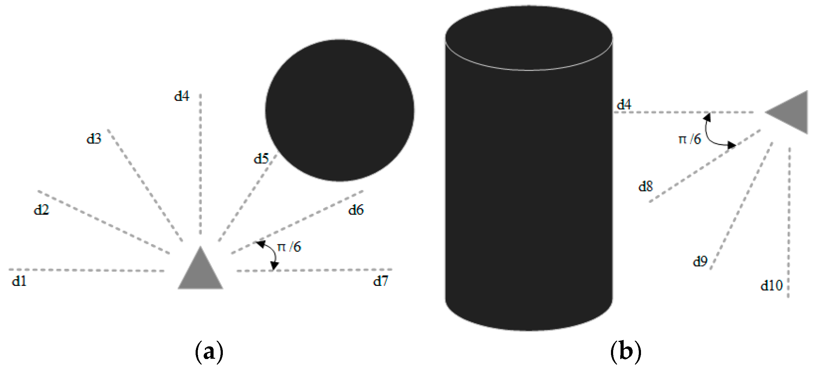
indicates the distance from the current position to the target point used to guide the UAV to approach the target point. , , and denote the current three-axis fractional velocity of the UAV. indicates the angle between the first view direction of the UAV and the direction of the line connecting the current position and the target point, as shown in Figure 1. This parameter is used to determine the degree of yaw of the UAV. Referring to the literature [19,24,25,30], we set the distance sensor in the form of Figure 2 for sensing obstacles. is the value of the blocked portion of the 10 onboard laser distance sensors and returns a value of 0 if not blocked by an obstacle; one sensor is set every . The sensors only need to be set in the front hemisphere in the forward direction of the UAV, where is distributed horizontally, as shown in Figure 2a, and is distributed vertically in the lower half of the circumference, as shown in Figure 2b. Because there are almost no obstacles during the upward flight of the UAV, there is no distance sensor set in the upper half of the vertical direction.
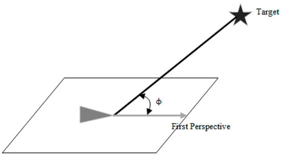
Figure 1.
Schematic diagram of the angle between the first view direction of UAV and the line connecting the current position and the target point; the triangle denotes UAV; the parallelogram is the flight plane in which the UAV is located, and the target point is not in the plane.
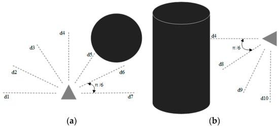
Figure 2.
Schematic diagram of the onboard distance sensor of the UAV, where triangles represent the UAV; circles and cylinders represent obstacles, and dashed lines represent distance sensors with fixed length; (a) shows the sensor distribution in the horizontal direction, and (b) shows the sensor distribution in the vertical direction.
Corresponding to the observation space, the action space in this study uses a three-axis distribution. To make the UAV freely control the flight speed and altitude, we use three-axis acceleration, , , , as action space. The acceleration of the three axes is added to the velocity of the three axes to change the current flight speed and control the motion of the UAV. As shown in Equation (4), rt indicates the time interval of each step. This design meets the requirements of adaptive control and does not cause sudden changes in the speed of the UAV, making the whole flight process smoother.
The objective of the reward function in this study is to guide the UAV to reach the target point as fast as possible while avoiding obstacles, which consists of six terms: distance reward; yaw penalty; obstacle penalty; target reward; collision penalty; and roaming penalty. To guide the UAV to the target point, the distance reward is designed as
The in (5) denotes the difference between the distance from the current position to the target point and the distance at the next step, which is calculated using (6). When the UAV advances toward a non-target point, a yaw penalty is applied. To help the UAV complete obstacle avoidance, the penalty is designed to be 0 within of yaw. When greater than , the larger the yaw angle is, the greater the penalty is, calculated as
To assist the UAV in avoiding obstacles, we apply an obstacle penalty to the UAV when it detects an obstacle within the minimum safe distance, calculated as
where is the maximum length of the blocked part of distance sensors, and safe is the threshold of the sensor that is blocked. The target reward and collision penalty are +25 and −25 when the UAV reaches the target point or a collision occurs. To guide the UAV to reach the target point as quickly as possible, we use a roaming penalty, where the UAV receives a penalty of −0.1 for each time step passed. The final reward obtained by the agent is the sum of the above reward functions.
In addition to the above three aspects, the flight altitude constraint, velocity constraint, and acceleration constraint are designed to make the UAV accomplish missions better and closer to the real environment. In terms of the flight altitude, the height ceiling is set in the simulation environment, which is a 250 environment-length unit. When the UAV touches the ceiling, it receives a penalty value equal to the collision penalty, guiding it to fly within a certain height range. The velocity constraint is implemented by designing the actor loss, and the acceleration constraint is achieved using the Tanh activation function, which will be described in detail in Section 3.
3. Method
3.1. TD3 and Layered-TD3
The basis of the GARTD3 algorithm is the twin delayed deep deterministic policy gradient (TD3) algorithm [31], an improved version of the deep deterministic policy gradient (DDPG) algorithm [32]. TD3 is a deterministic policy algorithm for continuous actions. Compared with the current strong random policy algorithms (e.g., A3C [33], PPO [34], SAC [35]) in the field of reinforcement learning, TD3’s advantages include the following:
- TD3 does not require the computational overhead of random sampling, which enhances its convergence;
- TD3 is an off-policy algorithm; its data can be divided into multiple state–action pairs and stored in the replay buffer, which has higher data utilization;
- TD3 can explore the boundary actions more easily, which is very beneficial in the UAV navigation problem, allowing for the model to adjust to the optimal flight speed faster.
Compared with another deterministic policy algorithm, D4PG [36], TD3 has a stronger stability, which is important in the observation and action space at high latitudes. And because the limited experimental equipment conditions do not support experiments using distributed reinforcement learning methods, we finally chose TD3 as the base algorithm. In terms of historical trajectories, we use LSTM and attention to process data within a fixed time window so that the UAV can obtain a more comprehensive perception of the surrounding environment from past historical experiences and enhance the UAV’s obstacle avoidance capability in complex low-altitude environments. The historical trajectory data consist of recent multi-step state–action pairs. Therefore, the base model of this paper is TD3, LSTM, and attention.
The TD3 algorithm introduces three main improvements to the DDPG algorithm: the use of double Q networks to solve the problem of overestimation; smooth normalization of the policy target network; and delayed update of the actor.
When the policy network is updated, the actor uses the Q value estimated by a critic to calculate the loss, and the Q value is often high, which will affect the update of the policy network. To solve this problem, there are two critic–target networks and two critic–online networks in the TD3 algorithm. The smaller Q value is selected to calculate the target value of critic–online, which is calculated as
The target policy network is regularized smoothly. To enable similar actions taken in the same state to have close values, the TD3 adds the cropped noise to the actions generated by the actor–target network so that a smoother action can be used to estimate the Q value in multiple updates. The corresponding calculation formula is
The actor’s update is delayed. Since the critic is constantly changing during the learning process, it is difficult for the actor to find the optimal strategy. Therefore, the TD3 uses the delayed actor update, which updates the actor after the critic has been updated several times to generate a more stable Q value.
The Layered-RTD3 algorithm applies the approach of the literature [24] to the TD3 algorithm, setting up an acquire module for navigation, an avoid module for obstacle avoidance, and a pack module for action selection, each part of which is implemented in RTD3 (using recurrent neural networks instead of fully connected networks). The Acquire module uses distance reward, yaw penalty, target reward, and roaming penalty as reward functions. Avoid module uses obstacle penalty and collision penalty as reward functions. The reward function of the Pack network is collision penalty as well as (11), which in , denotes the return length of each distance sensor; it is used to measure the degree of openness of the environment in which the UAV is located. The output of the pack module is a two-dimensional one-hot vector for selecting whether to perform navigation action or obstacle avoidance action. The final generated action is (12). The Critic part of the pack module is updated using the actions, whose update formula is (13) and (14), and the corresponding and are generated by the actor–target part of the avoid and acquire module.
3.2. Guide Attention
In this paper, we use three-axis acceleration to indirectly control the motion of the UAV and improve its flexibility. However, implementing this control method using TD3, LSTM, and attention, the convergence difficulty of the network is increased, which is directly manifested in the degradation of the UAV’s obstacle avoidance ability. In order to improve the obstacle avoidance ability of the algorithm in a low-altitude environment with multiple obstacles, the guide attention method is proposed. Unlike the familiar attention mechanism, guide attention is mainly implemented by feature engineering.
Autonomous UAV navigation is a multi-objective decision problem that requires performing both navigation and obstacle avoidance tasks at the same time. Therefore, to improve the obstacle avoidance capability, the UAV should shift its decision-making focus between navigation and obstacle avoidance, focusing more on the navigation task when it is in an environment with sparse obstacles and more on the obstacle avoidance task when it is in a complex environment with more obstacles. This is the core idea of guide attention.
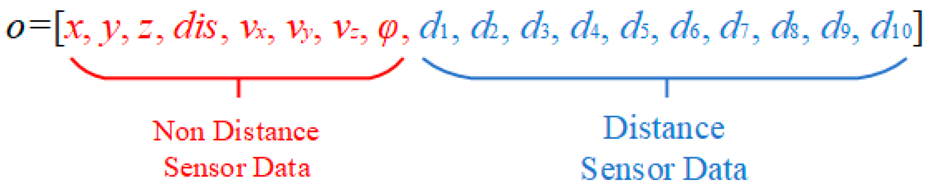
For this purpose, we analyze the observation data, which can be divided into two parts, as shown in Figure 3. The red part is the non-sensor data, which is mainly used to control the navigation of the UAV, and the blue part is the distance sensor data, which is the perception of obstacles for the UAV and is mainly used to control obstacle avoidance. The entire observation vector will be processed so that the decision focus shifts to the navigation direction or to the obstacle avoidance direction according to the observation value.
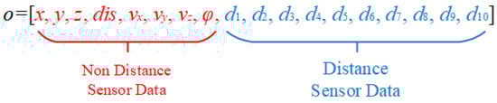
Figure 3.
Schematic diagram of observation data division.
First, we design a safety threshold for the distance sensor. The whole length of the sensor is set to . The original length of the distance sensor in this study is set to , and when the remaining length of the sensor is less than , an obstacle penalty is incurred.
Then, we divide the blue part of the distance sensor value by for normalization. When the occlusion value is less than , it is judged as a safe state (the surrounding obstacles are sparser), and when it is greater than , it is judged as an unsafe state, triggering the obstacle penalty. Based on this, we introduce the guide vector, whose length is equal to the observation vector. The first eight terms have a constant value of , and the last ten terms have a value of 1 minus the normalized result of the distance sensor reading. The vector is defined as
Thus, when the UAV is in an environment with many obstacles, the value of the sensor part of the vector is greater than and greater than the value of the non-sensor part, and the focus weight is shifted to the obstacle avoidance. When the UAV is in an environment with sparse obstacles, the value of the sensor part of the vector is lower than , which is lower than the value of the non-sensor part, and the focus weight is shifted to the navigation.
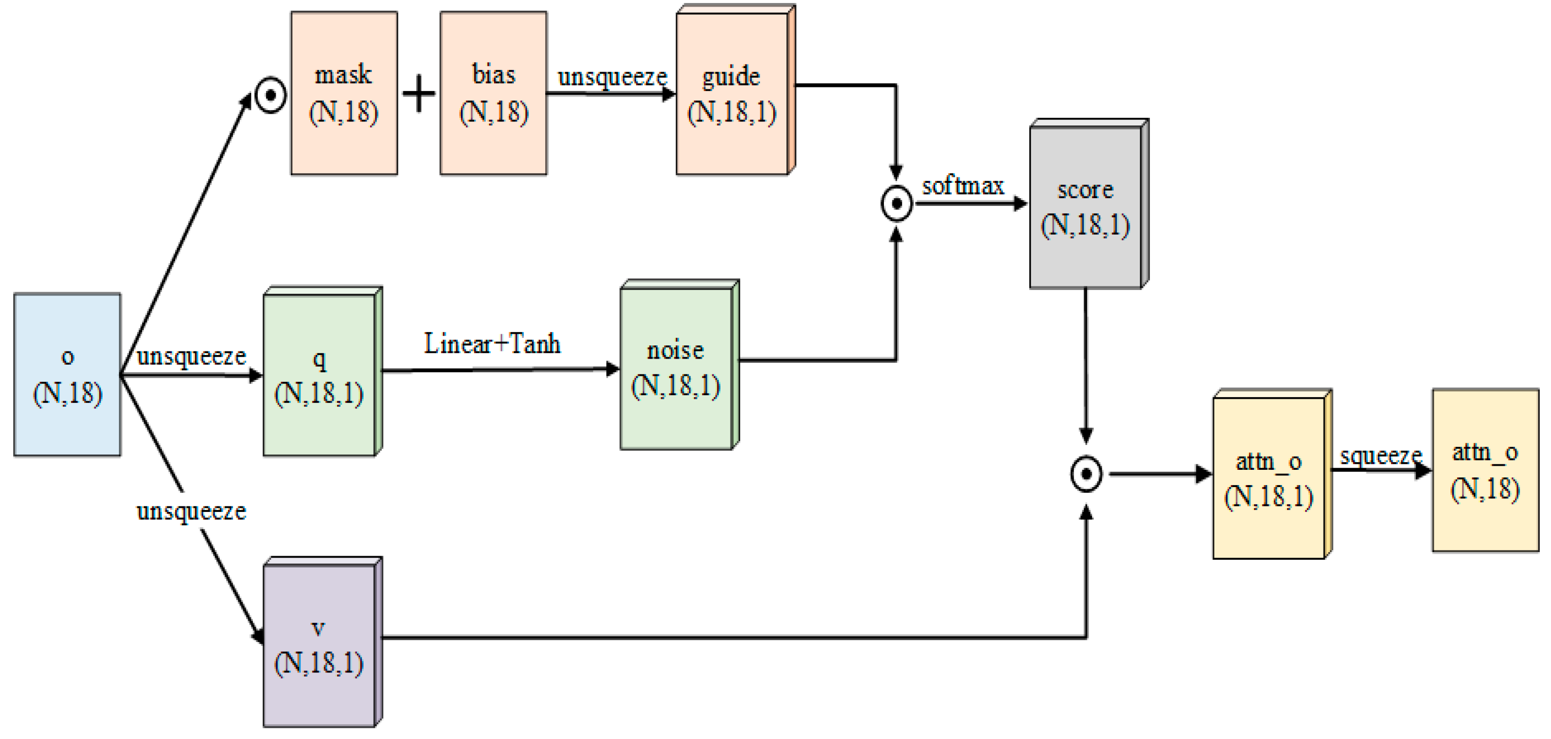
Finally, in order to enhance the accuracy of the guide vector to deal with complex situations and improve its fitting ability, we generate a noise vector from the observation, add it to the guide, and calculate the attention weights using the Softmax activation function. In this study, the above method is named guide attention, and the entire calculation process is as follows
The output of (16) is the attention weight, and noise is computed using (17). The specific process is as follows:
- Input the observation vector into the fully connected layer, using Relu as the activation function between layers;
- Use the tanh activation function as the output activation function to limit the value of noise and constrain its effect on the guide vector.
The guide vector (the current guide is batch data) is calculated using (18), which denotes the Hadamard Product. The values of mask and bias are shown in (19) and (20), and the number of rows of both matrices is equal to the batch size. The values of the first eight columns of the mask are 0, and the values of the last ten columns are 1. The values of the first eight columns of bias are ; the values of the last ten columns are 0. The first eight columns correspond to the non-sensor part of the data; the last ten columns correspond to the sensor part of the data. The weighted observation vector is obtained by multiplying attn and observation value with Hadamard Product. The weighted observation vector processed by guide attention is the input of the current observation of the entire algorithm.
In addition to enabling the UAV’s decision-making focus to be shifted according to its surroundings, guide attention also enhances the UAV’s perception of obstacle orientation. Traditional deep reinforcement learning algorithms for UAV navigation use reward functions to guide the UAV for obstacle avoidance; the obstacle avoidance penalty increases as the measurement from the shortest distance sensor decreases. This approach only allows the UAV to sense the impending collision and cannot determine exactly which direction the obstacle originates from, limiting its ability to avoid obstacles. But guide attention will only amplify the attention weight of the sensor that touches the obstacle, strengthening the judgment of the obstacle’s orientation and further enhancing the algorithm’s obstacle avoidance capability.
The internal structure of the guide attention module is shown in Figure 4. It is worth mentioning that in order to allow a critic to score state action pairs more rigorously, we only use the guide attention module to handle observation data in the actor.
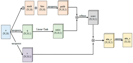
Figure 4.
The structure schematic diagram of guide attention, where the circle multiplication sign is the Hadamard Product.
3.3. Velocity-Constrained Loss Function
For the purpose of adaptive control, we use three-axis acceleration as the action space. However, using this approach would make the speed control of the UAV hard to learn, which largely increases the difficulty of obstacle avoidance. Therefore, we propose a novel exponential loss function to enhance the learning of speed control and add this loss function to the original loss function of the actor network.
The velocity-constrained loss function constructed in the GARTD3 algorithm is
In this loss function, denotes the component of the current velocity on the x-axis and y-axis; denotes the optimal velocity value with which the UAV can balance the navigation task and the obstacle avoidance task; this value is obtained from the statistics of our many experiments in the environment, and denotes the acceleration component generated by the actor network. The first term of the exponential partial product indicates the direction of the velocity, and the second term indicates the distance between the current velocity and the optimal velocity. During flight, the UAV tends to maintain a good velocity in the vertical direction, and the vertical velocity does not affect obstacle avoidance, so we only limit the velocity on the x and y-axes. When the partial velocity is at , the acceleration should be positive. Using this loss function, the closer it is to , the smaller the loss value is. When the partial velocity is at , the acceleration should be negative. Using this loss function, the closer it is to , the smaller the loss value is. In addition, the velocity-constrained loss is a convex function; the gradient decreases with the loss, which is more conducive to the optimization of the network parameters. Therefore, the loss function of the actor network can be modified as
where is the constraint coefficient, which is a hyperparameter.
Besides the two main improvements mentioned above, this paper also uses State Normalization to process the data in the navigation part of the observation vector. Every time a new piece of data is added to the replay buffer, the mean and standard deviation of all the data are calculated using a sliding average, and then, the currently added data are normalized to speed up the convergence of the network. In terms of network training, this paper uses course learning to first train the UAV in an environment with few obstacles and then keep increasing the obstacles in the environment. During this process, the UAV always needs to complete the navigation task in order to avoid forgetting what it has learned previously.
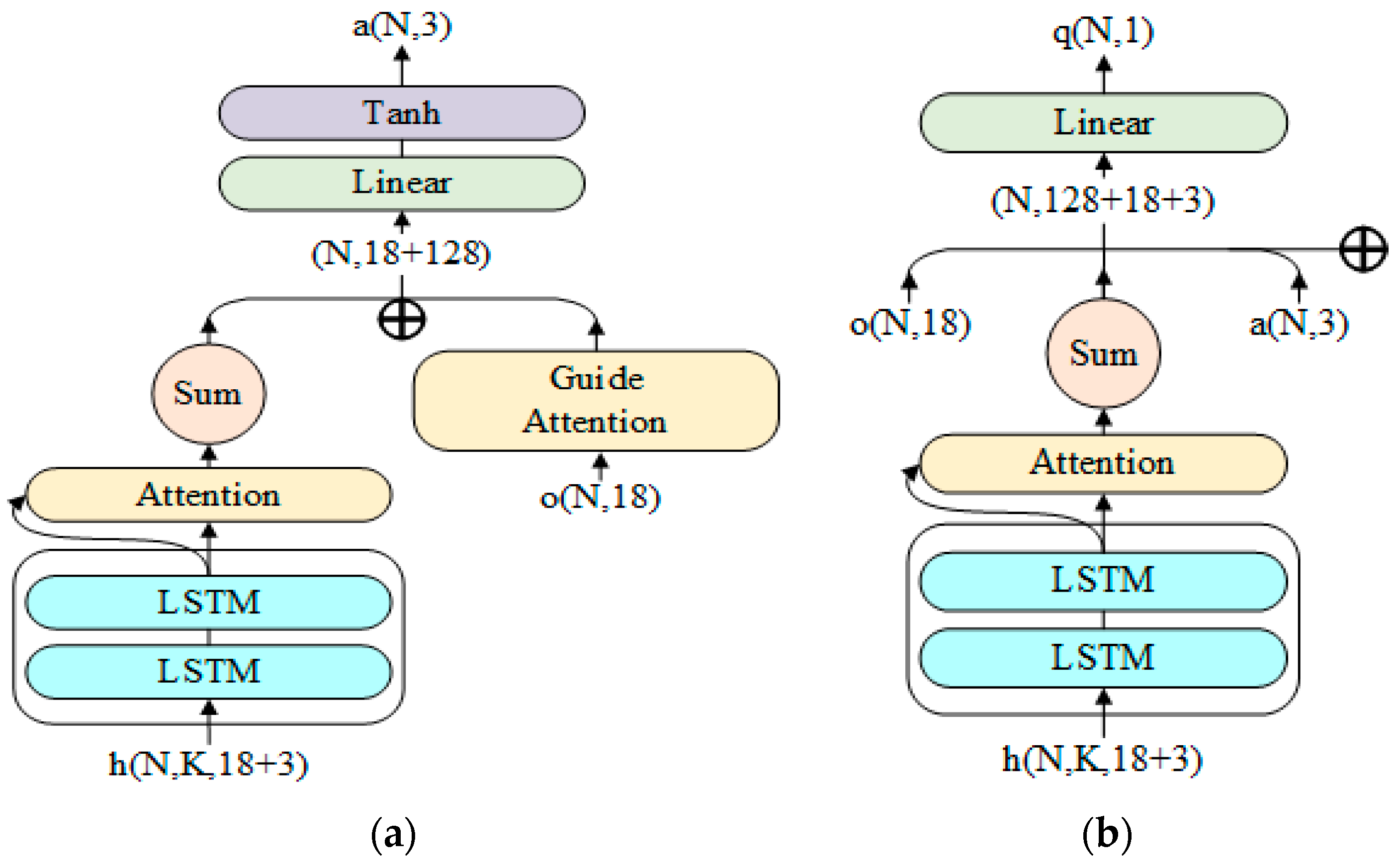
Finally, we incorporated them into the TD3 algorithm to obtain the GARTD3 algorithm and used LSTM and attention mechanism to extract features from historical trajectories in a fixed-length memory window. The pseudocode is shown in Algorithm 1. The structure of the actor and critic in the GARTD3 algorithm is shown in Figure 5a,b.
| Algorithm 1: Guide Attention Recurrent TD3 (GARTD3) |
| Initialize critic networks , , and actor network with random parameters , , Initialize target networks , , Initialize replay buffer . for to do Initialize memory window for to do Select action with exploration noise , , where calculating with (16)–(20), replacing with , reward and new observation Store transition tuple in Update with tuple Sample mini-batch of transitions from , Update critics using the gradient descent: if mod then: Update actor using the deterministic policy gradient: where calculate using (16)–(20), and replace with if then: if then: Update target networks: end for end for |
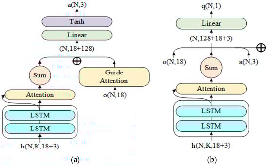
Figure 5.
Schematic diagram of the network model structure. (a) The network model structure of actor; its final output is an action vector with length of three. (b) Critic’s network model structure; the input is not processed by the Guide Attention module; is the output of actor, and the final output is the Q value.
4. Experiment
4.1. Simulation Environment
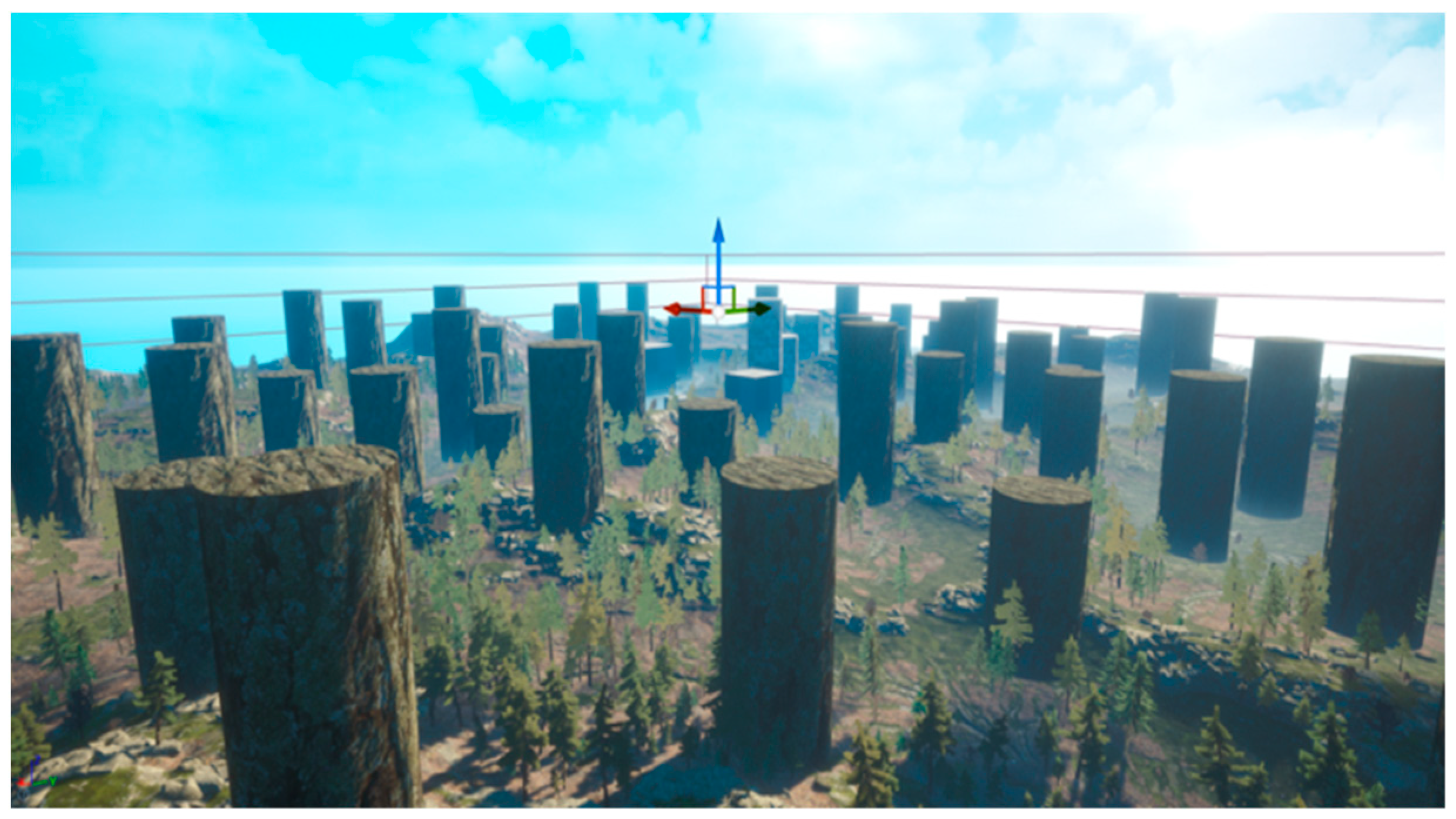
In this study, we use Unreal Engine 4 (UE4) and Airsim [37] to build a 3D simulation environment for training and testing algorithms. These tools provide a high-level control interface to the UAVs, eliminating the need for users to consider attitude adjustments while the UAVs are in flight and simplifying the experimental design. All experiments in this study are conducted in a 3D valley environment, which is a complex scene with lakes, jungles, mountains, rocks, and plains. To enhance the complexity of the experiments and demonstrate the obstacle avoidance capability of the GARTD3, we manually add multiple columnar obstacles of varying heights to the experimental environment. The 3D valley environment is shown in Figure 6.

Figure 6.
3D Valley Simulation Experimental Environment.
4.2. Experiment Setting
All experiments in this study use an NVIDIA GeForce RTX 3080 GPU (Santa Clara, CA, USA). To verify our proposed theory, the experiments are conducted in three aspects: the comparison of the GARTD3 algorithm with other algorithms; the effectiveness of the algorithm; and the effectiveness of the velocity-constrained loss function. The first two sets of experiments compare the GARTD3 with the TD3 and Layered-RTD3, and the third set of experiments compares the performance of the GARTD3 before and after using the velocity-constrained loss function in this study. All three algorithms use the observation space, action space, and reward function proposed in this paper; the recurrent neural network part of the Layered-RTD3 algorithm is LSTM.
Combined with the environment settings and the simulation experiment environment boundary, we define the experiment space as follows
The valley environment uses a three-axis coordinate system. The coordinate origin is the center of the environment, and the three positive directions point east, north, and earth. At the beginning of each episode, the UAV starts from the coordinate origin, and a target point randomly appears at any location in the experimental space. Because there are bulky obstacles in the valley, the target point may appear inside the terrain or obstacles. We design the success condition of the navigation mission as the Euclidean distance between the UAV and the target point is less than or equal to 25 m. If collisions occur, the current episode ends and the mission fails. Each artificially added obstacle in the environment is a cylinder, totaling 50 m, evenly and randomly distributed throughout the entire map, whose radius of the base is 25 m, and the height of a cylinder is a random number between 120 m and 170 m. The time interval for the UAV decision in the experiment is 0.5 s. The hyperparameters of the GARTD3 model are presented in Table 1. We trained 2500 episodes on the GARTD3, Layered-RTD3, and TD3 models in the same valley environment, and the saved models were tested for 150 episodes in an environment without noise.

Table 1.
The hyperparameters of GARTD3.
4.3. Comparison with Baseline
The test results of the GARTD3, Layered-RTD3, and TD3 algorithms are shown in Table 2. The bold represents the optimal value for each indicator. We compare the algorithms in terms of the average reward, the success rate of the task, and the collision rate. During the training process, we calculate the success rate of the final 100 and save the model corresponding to the episode with the highest success rate among them (the first 100 episodes are not saved). Table 2 records the average test results for the best model. Each algorithm is trained five times under different random seeds to obtain the average value to avoid the influence of random numbers. It can be seen that the GARTD3 algorithm’s average reward value is 59.12; the task success rate is 0.84, and the collision rate is only 0.16, with the average reward increasing by 9.35, the success rate of navigation tasks increasing by 14%, and the collision rate decreasing by 14%. Comparing the TD3 and Layered-RTD3 algorithms, the latter has a certain degree of improvement over the former in three aspects (average reward, success rate, and collision rate). It can be concluded that the introduction of historical trajectories can improve the performance of the algorithms in a 3D-complex environment. Compared with the Layered-RTD3 and TD3 algorithms, the GARTD3 algorithm is designed with a memory processing structure that is more conductive to extracting historical information. The use of guide attention and velocity-constrained loss function strengthens the algorithm’s obstacle avoidance and velocity control capability, so the GARTD3 algorithm can largely improve the performance of autonomous navigation. It is worth mentioning that at the beginning of the training phase, the models appeared to be unsuccessful or collided within 300 steps, but as the number of training episodes increased, this situation gradually disappeared, and none of the three models failed to reach the target point or collided within the specified 300 episodes at the time of testing, so the success rate and collision rate of the models combined was 1.0.
Table 2.
The comparison of the results of different algorithms.
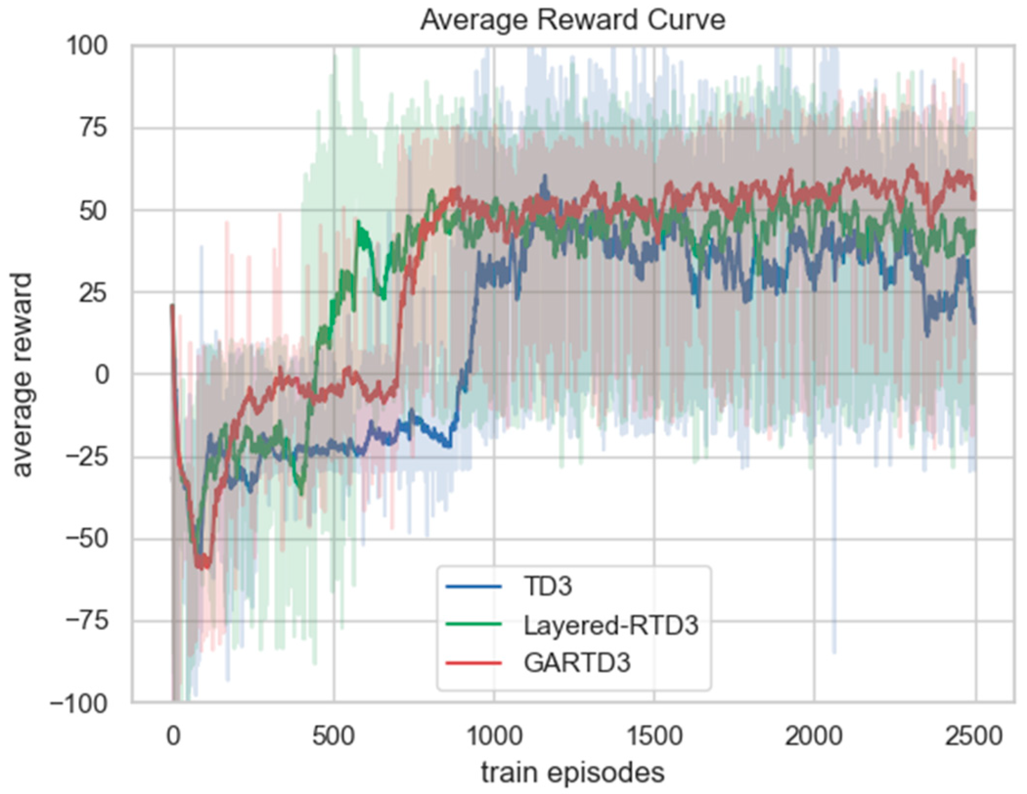
The average reward curve for each model during training is shown in Figure 7. The light part is the range of fluctuations of five different random seeds, and the dark part is the average curve. Both the GARTD3 and Layered-RTD3 algorithms converge at approximately 850 episodes, and the TD3 algorithm converges at approximately 1200 episodes. The GARTD3 algorithm converges faster than the original TD3 algorithm. The reason is that with the addition of the guide attention and velocity-constrained loss function, the GARTD3 can handle the complex environment better and fly out of a “terrain trap” faster, leaving the local optimum, while the TD3 algorithm will fall into the local optimum and need more training to fly out. Comparing the final convergence results of the curves, the average reward value of the GARTD3 algorithm is the highest, approximately 60, and both the TD3 and Layered-RTD3 algorithms are below 50. The convergence result of the Layered-RTD3 algorithm is higher than that of the TD3 algorithm, which proves that our proposed guide attention and velocity-constrained loss function can effectively improve a UAV’s obstacle avoidance ability and help it complete the task better and obtain a higher reward. In terms of the stability of the training curve, the GARTD3 algorithm has the best stability; the Layered-RTD3 algorithm is the second, and the TD3 algorithm has the worst stability among the three. This indicates that in a 3D complex environment, the GARTD3 algorithm can make the UAV learn a more stable and perfect navigation policy and have better results for different target points.

Figure 7.
The comparison graph of the average reward curve of different models during training. The average reward is the total reward value in an episode divided by the number of time steps. The light part is the range of fluctuations of 5 different random seeds, and the dark part is the average curve.
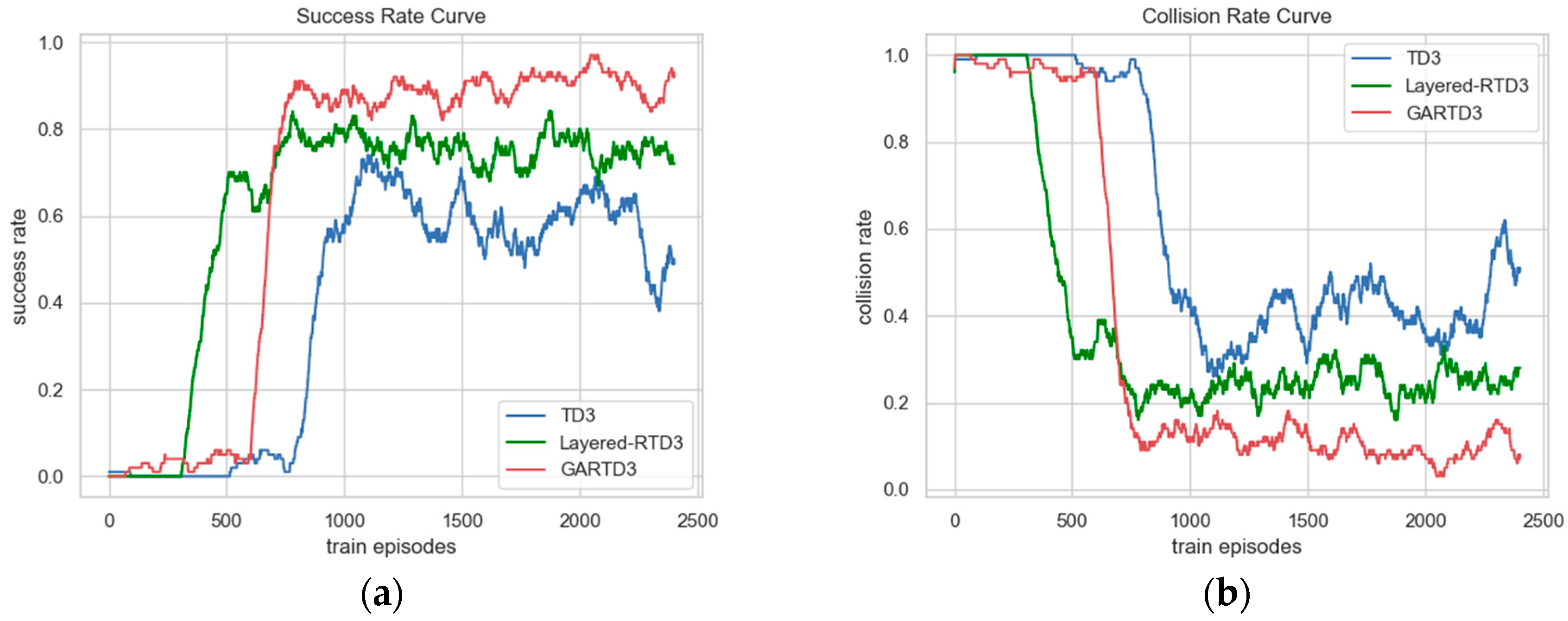
The task success and collision rate change curves during training are shown in Figure 8, where Figure 8a is the success rate change curve, and Figure 8b is the collision rate change curve, both of which are obtained by counting the success and collision of tasks in the last 100 episodes. The GARTD3 model ended up with a success rate of approximately 0.91; the Layered-RTD3 model was approximately 0.77, and the TD3 model had a success rate of approximately 0.65 until episode 2200, after which the success rate dropped to 0.5 due to the instability of network in complex environments. At the beginning of training, the model is unable to reach the target point, but this situation gradually disappears because of the roaming penalty, which forces the UAV to reach the target point as fast as possible. Figure 8 reflects that the convergence rates of the GARTD3 and Layered-RTD3 are comparable, and both are faster than the TD3 algorithm. The GARTD3 algorithm has the best convergence effect, and the success rate and collision rate both have a greater improvement compared to other algorithms within the same episode.
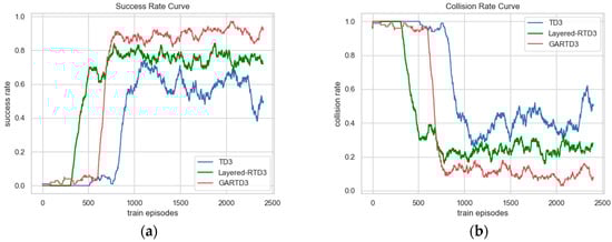
Figure 8.
The comparison of the success rate and collision rate change curves during training, both obtained by counting the number of successes and collisions at the last 100 episodes. (a) The success rate curve. (b) The collision rate curve.
4.4. Effectiveness of the GARTD3
In this subsection, we use the trained GARTD3, Layered-RTD3, and TD3 algorithms to perform navigation tasks in the 3D simulated valley environment to demonstrate the effectiveness of this algorithm.
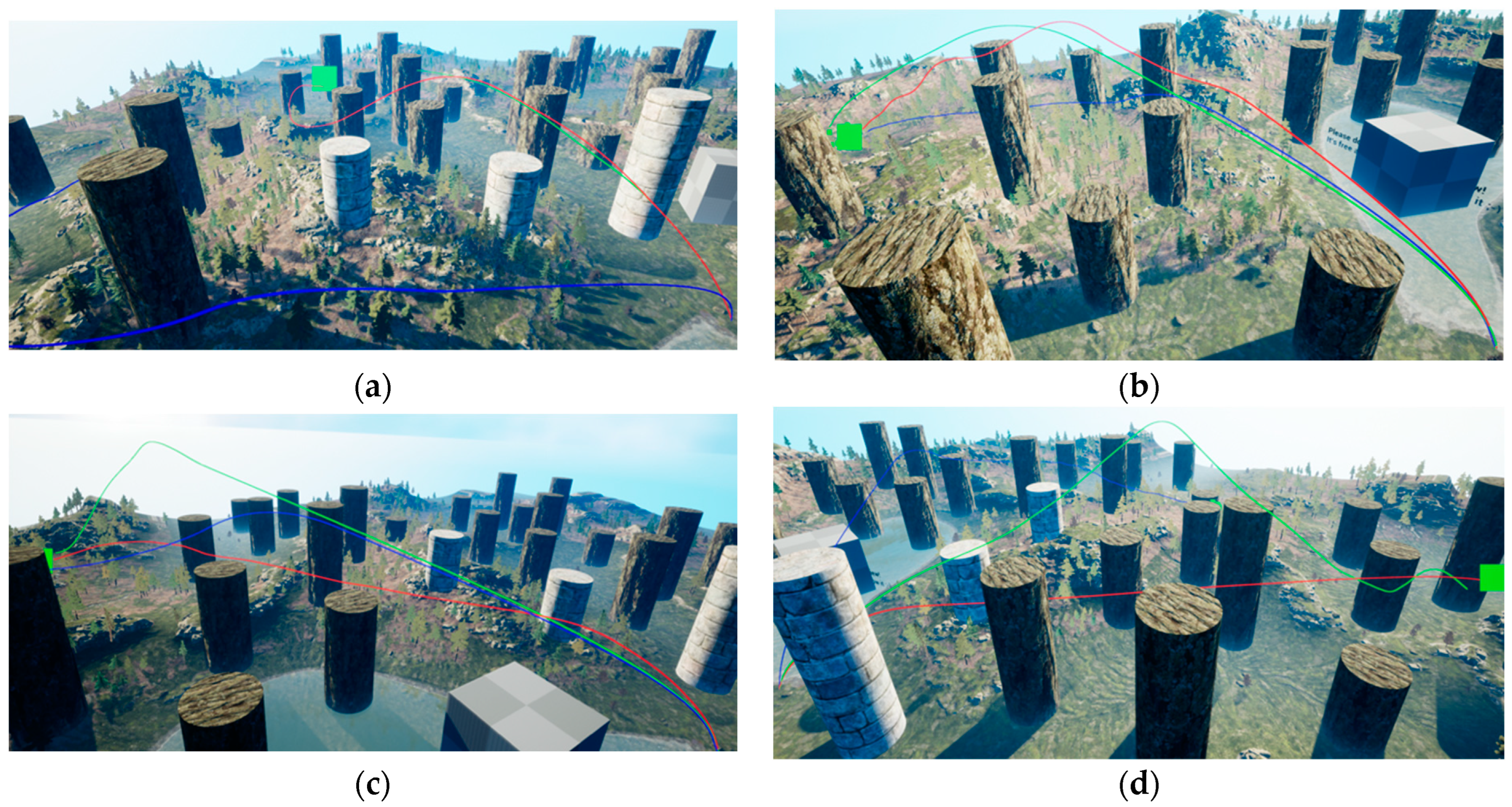
Figure 9 shows the flight trajectories of the UAV under the control of different algorithms for four different target points. The red trajectory is the result of the UAV flight under the control of GARTD3; the green trajectory is Layered-RTD3, and the blue one is TD3. The green square in the figure is the target location; the red curve is the UAV flight path, and the green point is the detection point of the distance sensor. Figure 9 shows that given that the flight altitude and velocity are not fixed, the UAV being trained using the GARTD3 algorithm can smoothly avoid multiple obstacles and reach the target point successfully with the shortest flight distance. The Layered-RTD3 algorithm trains a model with poor obstacle avoidance ability, which sometimes collides with an obstacle and obtains a longer flight range. The flight path of the UAV trained using the TD3 algorithm is not the optimal path and deviates from the direction of the target point, making it more likely to crash as well. The result demonstrates that our proposed GARTD3 algorithm can effectively improve the navigation ability and obstacle avoidance ability of UAVs in 3D-complex environments.
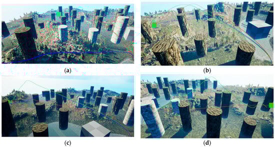
Figure 9.
The display diagram of the UAV navigation with different algorithms in the 3D valley environment. (a–d) displays flight routes for different target points.
4.5. Evaluating the Proposed Velocity-Constrained Loss Function
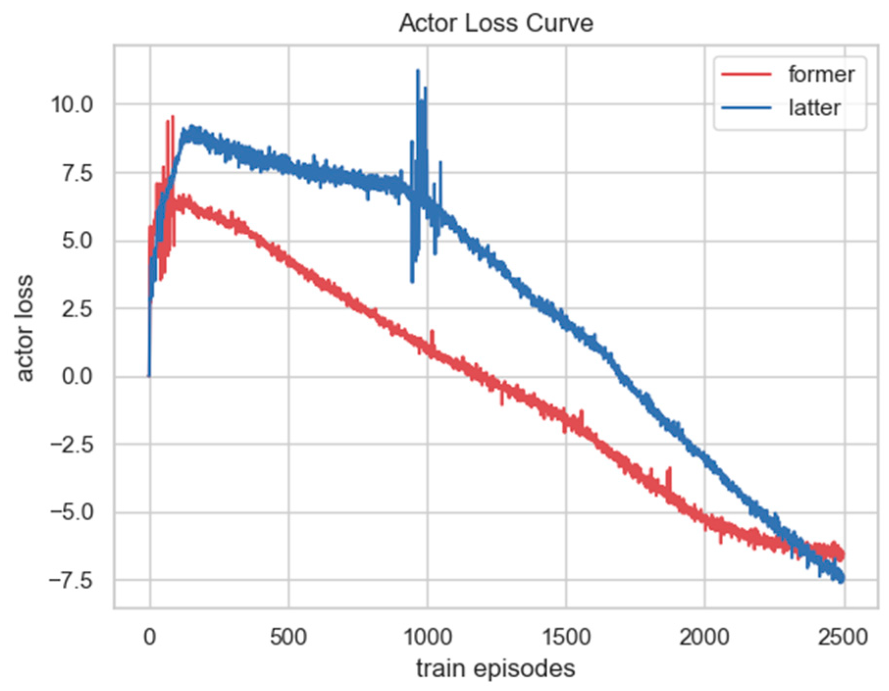
To verify the effect of the proposed velocity-constraint loss function, we compared the change in the actor loss of the GARTD3 algorithm before and after adding the velocity constraint during the training process, as shown in Figure 10. The red curve is the actor loss curve before adding the velocity-constrained function; the initial loss value is approximately 6, and the loss value converges to approximately −6 after 2500 training episodes. The blue curve is the actor loss curve after adding the constraint. Because the velocity constraint function is added, the initial loss value increases to approximately 9, and with the training of the model, the loss value drops to approximately −7.5 at 2500 episodes. There is still an obvious downward trend, indicating that the flight velocity of the UAV is also controlled well during the training process.
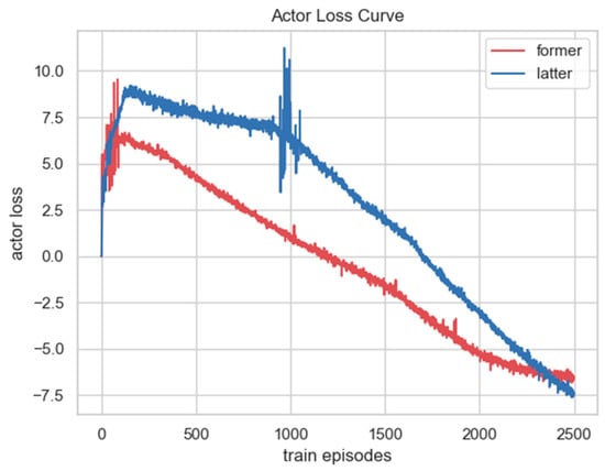
Figure 10.
The comparison of the actor loss change curve before and after adding the velocity-constrained function to the GARTD3 algorithm during training.
To demonstrate that the velocity-constrained loss function can stabilize the velocity near the optimal velocity, we compare the flight velocity change curves of GARTD3 before and after the addition of the loss function. As shown in Figure 11, , , and are the velocity change curves in the x, y, and z-axes, respectively, during the flight to the same target point; (a) is the image before adding the loss function, and (b) is the image after. The curve in (a) is highly volatile and more rugged. The curve in (b) is less volatile; it is smoother and has a smaller range of fluctuations. It follows that the velocity-constrained loss function strengthens the UAV’s speed control capabilities.
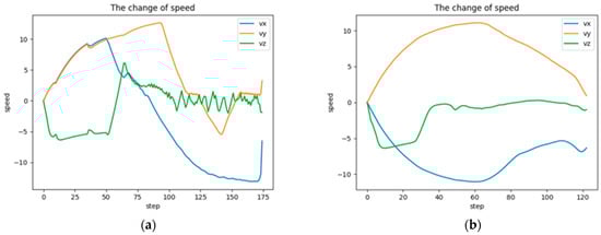
Figure 11.
The comparison of the speed change curve before and after adding the velocity-constrained function to the GARTD3 algorithm during training. (a) is the image before adding the loss function, and (b) is the image after.
Overall, compared to the advanced baselines, our proposed GARTD3 algorithm can largely improve the UAV’s navigation and obstacle avoidance capabilities in a 3D simulation environment and can more effectively control the flight speed. The algorithm also provides impressive results in terms of both convergence speed and stability.
5. Future Research Directions
Nevertheless, there are still some limitations to this research. We have not studied the navigation and obstacle avoidance strategies of drones in dynamic obstacles, and the diversity of cylindrical obstacles is insufficient. There are studies [38] that show that using non-convex obstacles such as circles and cylinders reduces the overall performance and validation efficiency of path planning and collision avoidance algorithms.
There is still some work to be accomplished in the future. Future research needs to improve the model’s ability to adapt to different environments so that the UAV can have excellent navigation and obstacle avoidance capabilities in any environment. Further developments to this study will use transfer learning algorithms to study how to deploy GARTD3 to real-world environments with dynamic obstacles. Future research will introduce computer visual algorithms to enhance the navigation ability of drones in dynamic environments and consider the impact of wind on the autonomous navigation of UAVs [39].
6. Conclusions
In this paper, we construct the UAV autonomous navigation with adaptive control in 3D complex environments as a POMDP model and propose the GARTD3 algorithm. To address the challenges of UAV navigation in low-altitude environments with multiple obstacles, we creatively propose a guide attention method so that the UAV can shift the decision focus between the navigation task and the obstacle avoidance task according to changes in the obstacle, which greatly improves the obstacle avoidance capability of the UAV. To solve the problem of speed control difficulties caused by adaptive flight, we raise a novel velocity-constrained loss function and add it to the original actor loss, which further improves the navigation capability of UAVs. Experiments show that in 3D simulation environments, the GARTD3 algorithm significantly improves the efficiency of the UAV, performing navigation tasks and obstacle avoidance ability and having good convergence and stability.
Author Contributions
Conceptualization, Z.W.; Methodology, Z.W., L.Z., Q.S. and Y.G.; Validation, Z.W.; Formal analysis, Z.W.; Visualization, Z.W.; Supervision, Y.Y.; Project administration, Y.Y.; Funding acquisition, Y.Y. All authors have read and agreed to the published version of the manuscript.
Funding
This research was funded by [Aviation Science Foundation] grant number [2022Z022051003].
Data Availability Statement
The experimental data comes from the interaction with the simulation environment, which is built using UE4 and Airsim. As our aviation fund project is not yet completed, simulation environment data is unavailable.
Conflicts of Interest
The authors declare no conflict of interest.
References
- Bokeno, E.T.; Bort, T.M.; Burns, S.S.; Rucidlo, M.; Wei, W.; Wires, D.L. Package Delivery by Means of an Automated Multicopter UAS/UAV Dispatched from a Conventional Delivery Vehicle. U.S. Patent 9,915,956, 13 March 2018. [Google Scholar]
- Grippa, P.; Behrens, D.A.; Bettstetter, C.; Wall, F. Job selection in a network of autonomous UAVs for delivery of goods. In Robotics: Science and Systems (RSS); MIT Press: Cambridge, MA, USA, 2017. [Google Scholar]
- Valenti, R.G.; Jian, Y.-D.; Ni, K.; Xiao, J. An autonomous flyer photographer. In Proceedings of the 2016 IEEE International Conference on Cyber Technology in Automation, Control, and Intelligent Systems, CYBER, Chengdu, China, 19–22 June 2016; pp. 273–278. [Google Scholar]
- Tomic, T.; Schmid, K.; Lutz, P.; Domel, A.; Kassecker, M.; Mair, E.; Grixa, I.L.; Ruess, F.; Suppa, M.; Burschka, D. Toward a fully autonomous UAV: Research platform for indoor and outdoor urban search and rescue. IEEE Robot. Autom. Mag. 2012, 19, 46–56. [Google Scholar] [CrossRef]
- Zhou, S.; Bai, C. Research on planetary rover path planning method based on deep reinforcement learning. J. Unmanned Veh. Syst. 2019, 2, 38–45. [Google Scholar]
- Duchoň, F.; Babinec, A.; Kajan, M.; Beňo, P.; Florek, M.; Fico, T.; Jurišica, L. Path planning with modified a star algorithm for a mobile robot. Procedia Eng. 2014, 96, 59–69. [Google Scholar] [CrossRef]
- Kala, R.; Warwick, K. Planning of multiple autonomous vehicles using rrt. In Proceedings of the 2011 IEEE 10th International Conference on Cybernetic Intelligent Systems, CIS, London, UK, 1–2 September 2011; pp. 20–25. [Google Scholar]
- Jayaweera, H.M.; Hanoun, S. A Dynamic Artificial Potential Field (D-APF) UAV Path Planning Technique for Following Ground Moving Targets. IEEE Access 2020, 8, 192760–192776. [Google Scholar] [CrossRef]
- Wang, Y.; Bai, P.; Liang, X.; Wang, W.; Zhang, J.; Fu, Q. Reconnaissance Mission Conducted by UAV Swarms Based on Distributed PSO Path Planning Algorithms. IEEE Access 2019, 7, 105086–105099. [Google Scholar] [CrossRef]
- Liu, Y.; Zhang, X.; Zhang, Y. Collision free 4D path planning for multiple UAVs based on spatial refined voting mechanism and PSO approach. Chin. J. Aeronaut. 2019, 32, 1504–1519. [Google Scholar] [CrossRef]
- Çalık, S.K. UAV path planning with multiagent Ant Colony system approach. In Proceedings of the 2016 24th Signal Processing and Communication Application Conference (SIU), Zonguldak, Turkey, 16–19 May 2016; pp. 1409–1412. [Google Scholar]
- Cheng, Z.; Sun, Y.; Liu, Y. Path planning based on immune genetic algorithm for UAV. In Proceedings of the 2011 International Conference on Electric Information and Control Engineering, Wuhan, China, 15–17 April 2011; pp. 590–593. [Google Scholar]
- Webb, D.J.; Van Den Berg, J. Kinodynamic rrt*: Asymptotically optimal motion planning for robots with linear dynamics. In Proceedings of the 2013 IEEE International Conference on Robotics and Automation, Karlsruhe, Germany, 6–10 May 2013; IEEE: New York, NY, USA, 2013; pp. 5054–5061. [Google Scholar]
- Bry, N.R. Rapidly-exploring random belief trees for motion planning under uncertainty. In Proceedings of the 2011 IEEE International Conference on Robotics and Automation, Shanghai, China, 9–13 May 2011; IEEE: New York, NY, USA, 2011; pp. 723–730. [Google Scholar]
- Nasir, J.; Islam, F.; Malik, U.; Ayaz, Y.; Hasan, O.; Khan, M.; Muhammad, M.S. RRT*-SMART: A rapid convergence implementation of RRT. Int. J. Adv. Robot. Syst. 2013, 10, 299. [Google Scholar] [CrossRef]
- Gammell, J.D.; Srinivasa, S.S.; Barfoot, T.D. Informed rrt*: Optimal sampling based path planning focused via direct sampling of an admissible ellipsoidal heuristic. In Proceedings of the 2014 IEEE/RSJ International Conference on Intelligent Robots and Systems, Chicago, IL, USA, 14–18 September 2014; IEEE: New York, NY, USA, 2014; pp. 2997–3004. [Google Scholar]
- Liu, S.; Atanasov, N.; Mohta, K.; Kumar, V. Search-based motion planning for quadrotors using linear quadratic minimum time control. In Proceedings of the 2017 IEEE/RSJ International Conference on Intelligent Robots and Systems, IROS, Vancouver, BC, USA, 24–28 September 2017; IEEE: New York, NY, USA, 2017; pp. 2872–2879. [Google Scholar]
- Razzaghi, P.; Tabrizian, A.; Guo, W.; Chen, S.; Taye, A.; Thompson, E.; Bregeon, A.; Ba-heri, A.; Wei, P. A survey on reinforcement learning in aviation applications. arXiv 2022, arXiv:2211.02147. [Google Scholar]
- Wang, C.; Wang, J.; Shen, Y.; Zhang, X. Autonomous Navigation of UAVs in Large-Scale Complex Environments: A Deep Reinforcement Learning Approach. IEEE Trans. Veh. Technol. 2019, 68, 2124–2136. [Google Scholar] [CrossRef]
- Heess, N.; Hunt, J.J.; Lillicrap, T.P.; Silver, D. Memory-based control with recurrent neural networks. arXiv 2015, arXiv:1512.04455. [Google Scholar]
- Fu, C.; Xu, X.; Zhang, Y.; Lyu, Y.; Xia, Y.; Zhou, Z.; Wu, W. Memory-enhanced deep reinforcement learning for UAV navigation in 3D environment. Neural Comput. Appl. 2022, 34, 14599–14607. [Google Scholar] [CrossRef]
- Mnih, V.; Kavukcuoglu, K.; Silver, D. Human-level control through deep reinforcement learning. Nature 2015, 518, 529. [Google Scholar] [CrossRef] [PubMed]
- Singla, A.; Padakandla, S.; Bhatnagar, S. Memory-Based Deep Reinforcement Learning for Obstacle Avoidance in UAV With Limited Environment Knowledge. IEEE Trans. Intell. Transp. Syst. 2021, 22, 107–118. [Google Scholar] [CrossRef]
- Zhang, S.; Li, Y.; Dong, Q. Autonomous navigation of UAV in multi-obstacle environments based on a Deep Reinforcement Learning approach. Appl. Soft Comput. 2022, 115, 108194. [Google Scholar] [CrossRef]
- Guo, T.; Jiang, N.; Li, B.; Zhu, X.; Wang, Y.; Du, W. UAV navigation in high dynamic environments: A deep reinforcement learning approach. Chin. J. Aeronaut. 2021, 34, 2. [Google Scholar] [CrossRef]
- Hu, J.; Yang, X.; Wang, W.; Wei, P.; Ying, L.; Liu, Y. Obstacle avoidance for uas in continuous action space using deep reinforcement learning. IEEE Access 2022, 10, 90623–90634. [Google Scholar] [CrossRef]
- Schaul, T.; Quan, J.; Antonoglou, I.; Silver, D. Prioritized experience replay. arXiv 2016, arXiv:1511.05952. [Google Scholar]
- Hu, Z.J.; Gao, X.G.; Wan, K.F.; Zhai, Y.W.; Wang, Q.L. Relevant experience learning: A deep reinforcement learning method for UAV autonomous motion planning in complex unknown environments. Chin. J. Aeronaut. 2021, 34, 187–204. [Google Scholar] [CrossRef]
- Loquercio, A.; Maqueda, A.I.; Del-Blanco, C.R.; Scaramuzza, D. Dronet: Learning to flfly by driving. IEEE Robot. Autom. Lett. 2018, 3, 1088–1095. [Google Scholar] [CrossRef]
- Wang, C.; Wang, J.; Wang, J.; Zhang, X. Deep-Reinforcement-Learning-Based Autonomous UAV Navigation with Sparse Rewards. IEEE Internet Things J. 2020, 7, 6180–6190. [Google Scholar] [CrossRef]
- Fujimoto, S.; Hoof, H.; Meger, D. Addressing function approximation error in actor-critic methods. In Proceedings of the International Conference on Machine Learning, PMLR, Stockholm, Sweden, 10–15 July 2018; pp. 1587–1596. [Google Scholar]
- Lillicrap, T.P.; Hunt, J.J.; Pritzel, A.; Heess, N.; Erez, T.; Tassa, Y.; Silver, D.; Wierstra, D. Continuous control with deep reinforcement learning. arXiv 2019, arXiv:1509.02971. [Google Scholar]
- Mnih, V.; Badia, A.P.; Mirza, M.; Graves, A.; Lillicrap, T.; Harley, T.; Silver, D.; Kavukcuoglu, K. Asynchronous methods for deep reinforcement learning. In Proceedings of the 33rd International Conference on Machine Learning (ICML), New York, NY, USA, 20–22 June 2016; pp. 1928–1937. [Google Scholar]
- Schulman, J.; Wolski, F.; Dhariwal, P.; Radford, A.; Klimov, O. Proximal policy optimization algorithms. arXiv 2017, arXiv:1707.06347. [Google Scholar]
- Haarnoja, T.; Zhou, A.; Abbeel, P.; Levine, S. Soft actor-critic: Off-policy maximum entropy deep reinforcement learning with a stochastic actor. In Proceedings of the 35th International Conference on Machine Learning, ICML, Stockholm, Sweden, 10–15 July 2018; Volume 5, pp. 2976–2989. [Google Scholar]
- Barth-Maron, G.; Hoffman, M.W.; Budden, D.; Dabney, W.; Horgan, D.; Tb, D.; Muldal, A.; Heess, N.; Lillicrap, T. Distributed distributional deterministic policy gradients. arXiv 2018, arXiv:1804.08617. [Google Scholar]
- Shah, S.; Dey, D.; Lovett, C.; Kapoor, A. AirSim: High-Fidelity Visual and Physical Simulation for Autonomous Vehicles. arXiv 2017, arXiv:1705.05065. [Google Scholar]
- Phadke, A.; Medrano, F.A.; Chu, T.; Sekharan, C.N.; Starek, M.J. Modeling Wind and Obstacle Disturbances for Effective Performance Observations and Analysis of Resilience in UAV Swarms. Aerospace 2024, 11, 237. [Google Scholar] [CrossRef]
- Jayaweera, H.M.P.C.; Hanoun, S. Path Planning of Unmanned Aerial Vehicles (UAVs) in Windy Environments. Drones 2022, 6, 101. [Google Scholar] [CrossRef]

Disclaimer/Publisher’s Note: The statements, opinions and data contained in all publications are solely those of the individual author(s) and contributor(s) and not of MDPI and/or the editor(s). MDPI and/or the editor(s) disclaim responsibility for any injury to people or property resulting from any ideas, methods, instructions or products referred to in the content. |
© 2024 by the authors. Licensee MDPI, Basel, Switzerland. This article is an open access article distributed under the terms and conditions of the Creative Commons Attribution (CC BY) license (https://creativecommons.org/licenses/by/4.0/).