Diffusion-Based Radio Signal Augmentation for Automatic Modulation Classification

Abstract

Deep learning has become a powerful tool for automatically classifying modulations in received radio signals, a task traditionally reliant on manual expertise. However, the effectiveness of deep learning models hinges on the availability of substantial data. Limited training data often results in overfitting, which significantly impacts classification accuracy. Traditional signal augmentation methods like rotation and flipping have been employed to mitigate this issue, but their effectiveness in enriching datasets is somewhat limited. This paper introduces the Diffusion-based Radio Signal Augmentation algorithm (DiRSA), a novel signal augmentation method that significantly enhances dataset scale without compromising signal integrity. Utilizing prompt words for precise signal generation, DiRSA allows for flexible modulation control and significantly expands the training dataset beyond the original scale. Extensive evaluations demonstrate that DiRSA outperforms traditional signal augmentation techniques such as rotation and flipping. Specifically, when applied with the LSTM model in small dataset scenarios, DiRSA enhances modulation classification performance at SNRs above 0 dB by 6%.

1. Introduction

Automatic modulation classification (AMC) is a pivotal technology in wireless communications that is designed to automatically categorize the modulation categories of received radio signals. Modulation techniques, the method by which information is encoded for transmission, vary widely, each with distinct advantages, applications, and suitability for different communication environments. Common modulation schemes, such as continuous-phase frequency shift keying (CPFSK), amplitude modulation double sideband (AM-DSB), Gaussian frequency-shift keying (GFSK), M-phase-shift keying (MPSK), M-quadrature amplitude modulation (MQAM), and wideband frequency modulation (WBFM), have been extensively used due to their robustness and effectiveness in traditional communication systems. However, emerging modulation techniques such as chaotic modulation [1] and orthogonal time frequency space (OTFS) modulation [2] are gaining attention for their potential to enhance signal robustness and spectral efficiency in highly dynamic environments. The diverse range of available modulation techniques reflects the evolving landscape of wireless technology, where the choice of modulation can significantly impact the efficiency, reliability, and security of the communication system. Understanding and classifying these modulation categories accurately is therefore of paramount importance for the design and optimization of next-generation wireless communication systems. This backdrop sets the stage for our investigation into AMC, as it seeks to harness deep learning algorithms to automatically identify and adapt to various modulation schemes, further enhancing the capabilities of cognitive radios and adaptive communication systems. The ability to accurately and efficiently discern modulation categories is crucial not only for the operation of modern communication systems [3,4] but also for the significant role it plays in advancing areas such as cognitive radio [5], spectrum monitoring [6], and electronic warfare [7].

Currently, AMC has branched into three principal methodologies: likelihood theory-based (LB) methods, feature extraction (FB) methods [8], and deep learning-based (DL) methods [9]. LB methods, while precise under controlled conditions, often fail to perform well in real-world scenarios due to their high sensitivity to noise and signal distortions. In contrast, FB methods, though effective in extracting key signal features, are limited by their inability to dynamically adapt to the variability and complexity of modern communication signals. Compared with DL methods, which can automatically extract signal features, the first two methods appear somewhat outdated. Therefore, the research interest in the first two has subsided, with deep learning-based methods now at the forefront of ongoing progress in the field. Recent advancements in deep learning, particularly in convolutional neural networks (CNNs) [10], recurrent neural networks (RNNs) [11], and other models [12], have significantly enhanced AMC’s capabilities. It is illustrated that radio features extracted by deep learning models are similar to the knowledge of human experts [13]. Therefore, DL has now become the mainstream pipeline for AMC [14].

Yet, despite their promise, the success of deep learning models hinges on the availability of large datasets. Insufficient data can result in overfitting, diminishing the model’s practical applicability. Previous studies show that small datasets limit the complexity of deep learning models, and training more complex models on small datasets will have negative effects [15]. And, for real-world problems, massive training samples are difficult to obtain in non-cooperative scenarios [16,17]. Therefore, research on signal augmentation of small datasets is crucial to face the challenges associated with data scarcity. Traditional signal augmentation techniques, such as signal rotation and flipping [18], have been employed to increase the scale of training datasets, which helps mitigate overfitting. However, these methods are limited in the scale of augmentation they can achieve, typically up to 7×, resulting in a capped improvement in performance. Generative models, including generative adversarial networks (GANs) [19], are utilized for signal augmentation in the field of AMC. However, compared to rotation and flipping, the scale of augmentation achieved by GANs is relatively modest, and the resulting augmentation effect is considered to be average.

In this paper, we introduce DiRSA, a novel solution engineered to significantly enhance the performance and applicability of diffusion models in signal augmentation and AMC. DiRSA skillfully adapts the diffusion denoising probabilistic model (DDPM) framework [20] to meet the unique challenges present in AMC. By integrating masking with conditional probabilities, DiRSA extends the DDPM’s capabilities to effectively handle complex radio signals, allowing for partial reconstruction and signal augmentation. To guide the modulation category of the augmented signals, we novelly introduce prompt words into DiRSA. This feature enables the precise and flexible generation of signal segments corresponding to specific modulation categories. The augmented datasets generated by DiRSA facilitate the training of AMC models that demonstrate markedly improved accuracy, as verified through thorough testing and evaluation. The main contributions of this paper are summarized as follows:

• A novel signal augmentation algorithm, DiRSA, which significantly augments the volume of training data available for AMC models without compromising the intrinsic qualities of the radio signals.
• By incorporating prompt words, the DiRSA technique enhances the accuracy of generating signal data for specific modulation categories, effectively reducing the potential for the confusion commonly associated with generative models. This approach is more adaptable compared to the plain method of training separate models for each modulation category. Utilizing prompt words to dictate the modulation category of generated signals not only simplifies the control mechanism but also significantly decreases the number of model files required, thereby facilitating easier management.
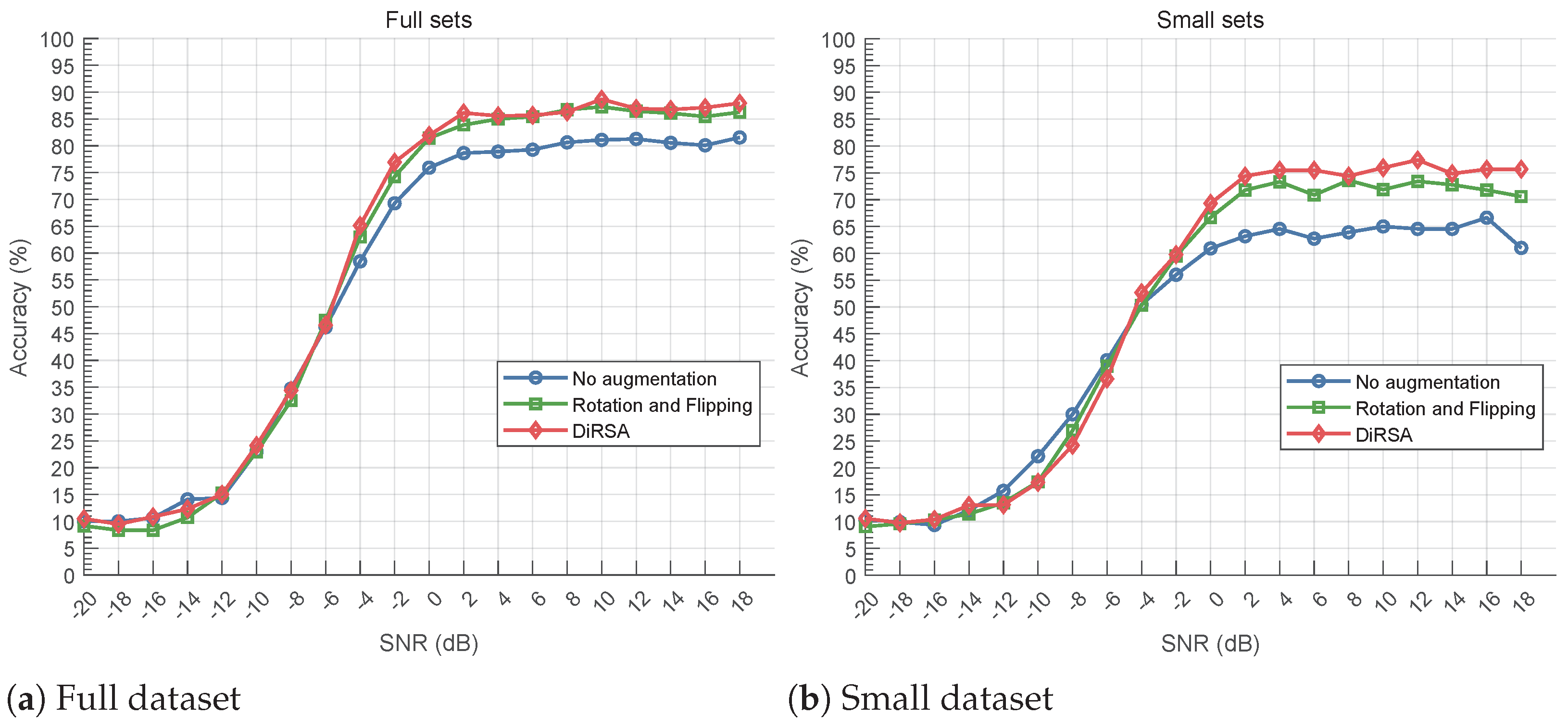
• Compared to traditional signal augmentation methods, such as rotation and flipping, DiRSA-augmented datasets can achieve more effective modulation classification performance. When using long short-term memory (LSTM) [21], CNNs, and convolutional long short-term memory fully connected deep neural networks (CLDNNs) [22], DiRSA performs 2.75–5.92% better than rotation and flipping in small dataset scenarios at an SNR higher than 0 dB.

2. The DiRSA

In this section, we present the DiRSA, including the architecture of DiRSA, its prompt-based denoising process, and its self-supervised training method.

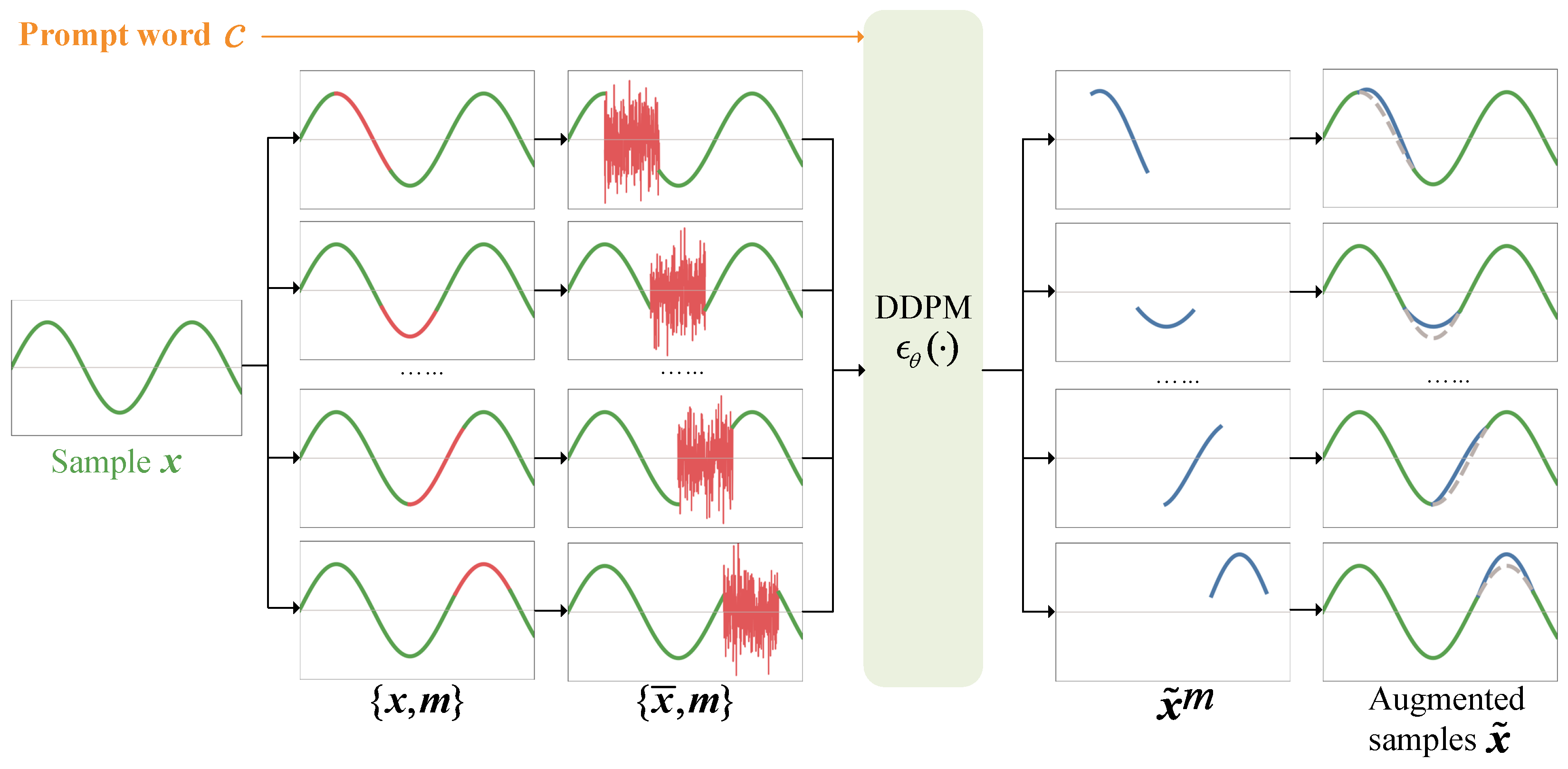
2.1. Overview of DiRSA

DiRSA innovatively generates new signal samples by reconstructing segments of existing signals from random noise, guided by prompt words that specify the target modulation category. This process facilitates the expansion of signal datasets for training deep learning models, consequently enhancing AMC accuracy. The architecture of DiRSA, depicted in Figure 1, includes signal masking, signal denoising, and signal embedding:

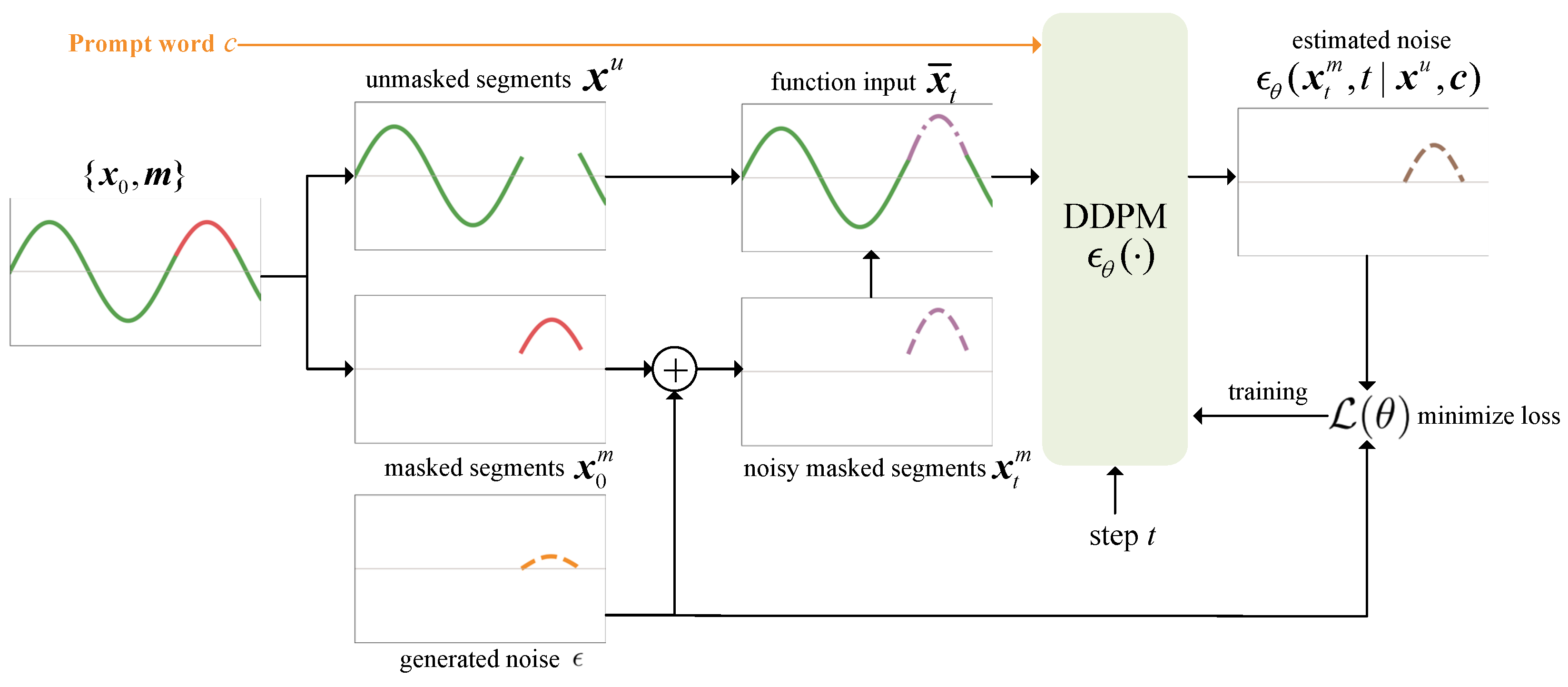
• Signal masking. Starting with a sample of radio signals $\mathit{x}=\{x_i\mid i\in \{1,2,\dots ,L\}\}\in {\mathbb{R}}^L$, where L is the length of the sample, we apply a mask $\mathit{m}=\{m_i\mid i\in \{1,2,\dots ,L\}\}\in {\{0,1\}}^L$. This mask ensures that $L_m$ consecutive elements are set to 1. Each masked signal sample $\mathit{x}$ is then split into a masked segment ${\mathit{x}}^m=\{x_i\mid m_i=1\}$ and unmasked segments ${\mathit{x}}^u=\{x_i\mid m_i=0\}$. As depicted in Figure 1, the masked segments are shown with red lines, while the unmasked segments are displayed with green lines. The masked segments ${\mathit{x}}^m$ are replaced with pure noise from a standard Gaussian distribution $\mathcal{N}(0,1)$, resulting in a new noised signal sample $\overline{\mathit{x}}$.
• Signal denoising. An adapted DDPM is employed to reconstruct the signal ${\tilde{\mathit{x}}}^m$ from the noise. This process is influenced by a prompt word vector $\mathit{c}$, representing the modulation category’s one-hot encoding. The pair $\{\overline{\mathit{x}},\mathit{m}\}$ and the prompt word $\mathit{c}$ are input into the DDPM, which outputs ${\tilde{\mathit{x}}}^m$, approximating ${\mathit{x}}^m$ based on the unmasked segments ${\mathit{x}}^u$.
• Signal embedding. The reconstructed segment ${\tilde{\mathit{x}}}^m$ is then embedded back into the original signal sample $\mathit{x}$ by replacing the original masked segment. This produces a new augmented signal sample $\tilde{\mathit{x}}$, shown as blue solid lines in Figure 1, with the original ${\mathit{x}}^m$ depicted as gray dotted lines.

For each radio signal sample in the original dataset, we generate K different masks and repeat the DiRSA process K times, effectively augmenting the original dataset by a factor of K. This expansion coefficient, K, significantly enhances the diversity and volume of data available for training AMC models.

2.2. Prompt-Based Signal Denoising

To improve the suitability of diffusion models for signal processing, especially in addressing the unique challenges of AMC, DiRSA implements substantial modifications to the DDPM framework [20]. These modifications are crafted to enhance performance and specificity in signal reconstruction and to enable the application of diffusion models for signal augmentation within the AMC domain. The details are as follows:

• Masking and conditional probability: DiRSA employs a novel approach that utilizes masking alongside conditional probabilities. This method allows DiRSA to adapt to IQ signal data and enables the reconstruction of the remaining noise portions of a signal into newly suitable signal segments based on the features of the non-noise portions, thereby achieving the effect of signal augmentation.
• Prompt word for modulation category: Uniquely, DiRSA incorporates the modulation category as a prompt word within its process. Each sample that requires signal augmentation will have a modulation category. It is assigned a unique identifier that ranges from 0 to 10. These identifiers are then transformed into a one-hot encoding format, where each identifier is represented by an 11-element binary vector. In this vector, only the position corresponding to the identifier is marked as “1”, with all other positions set to “0”. This one-hot encoded vector is subsequently used as a prompt word in the input to our model. This innovation allows for the stable generation of signal data corresponding precisely to the specified modulation category. By doing so, DiRSA enhances its utility and accuracy in the field of automatic modulation classification, ensuring that the generated signals are consistently aligned with the desired modulation features.

2.2.1. Denoising Process

DiRSA’s denoising process unfolds over $T=50$ steps, where the noise signal sample $\overline{\mathit{x}}$ is gradually denoised to the augmented signal sample $\tilde{\mathit{x}}$. We denote ${\overline{\mathit{x}}}_t$ as the resulting signal sample at step t, for all $t=T,T-1,\cdots ,0$. We define ${\overline{\mathit{x}}}_T=\overline{\mathit{x}}$, ${\overline{\mathit{x}}}_0=\tilde{\mathit{x}}$, and ${\mathit{x}}_t^m$ as the masked segment of ${\overline{\mathit{x}}}_t$. This transformation through denoising is depicted in Figure 2. As an example, we illustrate the first two steps of the prompt-based denoising process in Figure 2a. When $t=T$, we input $\{{\overline{\mathit{x}}}_T,\mathit{m}\}$ into a noise estimation function, ${ϵ}_{\theta }(·)$, which estimates the noise at the current step based on unmasked segments ${\mathit{x}}^u$ and the prompt word $\mathit{c}$, resulting in ${ϵ}_{\theta }({\mathit{x}}_T^m,T|{\mathit{x}}^u,\mathit{c})$. We then subtract the estimated noise from ${\overline{\mathit{x}}}_T$ and obtain ${\overline{\mathit{x}}}_{T-1}$ for the next step. We then input $\{{\overline{\mathit{x}}}_{T-1},\mathit{m}\}$ into the noise estimation function again, estimate the noise at $t=T-1$ as ${ϵ}_{\theta }({\mathit{x}}_{T-1}^m,t|{\mathit{x}}^u,\mathit{c})$, and obtain ${\overline{\mathit{x}}}_{T-2}$. By iterating all steps $t=T,T-1,\cdots ,0$, we obtain the denoised signal sample, ${\overline{\mathit{x}}}_0$, as shown in Figure 2b.

The core concept of the DDPM involves learning a model distribution $p_{\theta }(·)$ that closely approximates a given data distribution $q(·)$. The latter will be elaborated in detail in Section 2.3. Upon the model approximation, the key step in the denoising process is the recovery of the data distribution of ${\mathit{x}}_{t-1}^m$ from ${\mathit{x}}_t^m$, which is assumed to be a Gaussian diffusion process, as

$$p_{\theta }\left({\mathit{x}}_{t-1}^m\right|{\mathit{x}}_t^m,{\mathit{x}}^u,\mathit{c}):=\mathcal{N}({\mathit{x}}_{t-1}^m;{\mu }_{\theta }({\mathit{x}}_t^m,t|{\mathit{x}}^u,\mathit{c}),{\sigma }_{\theta }\left(t\right)\mathit{I}),$$

(1)

where ${\mu }_{\theta }$ and ${\sigma }_{\theta }$ are adapted from Ho et al. [20], the conditional ${\mathit{x}}^u$ is adopted from Tashiro et al. [23], and the conditional prompt word $\mathit{c}$ is newly introduced to fit the modulation label. Specifically, we have

$${\mu }_{\theta }({\mathit{x}}_t^m,t|{\mathit{x}}^u,\mathit{c})=\frac{1}{{\alpha }_t}\left({\mathit{x}}_t^m-\frac{{\beta }_t}{\sqrt{1-{\alpha }_t}}{ϵ}_{\theta }({\mathit{x}}_t^m,t|{\mathit{x}}^u,\mathit{c})\right),$$

(2)

and

$$\begin{array}{c}\hfill {\sigma }_{\theta }\left(t\right)=\sqrt{{\tilde{\beta }}_t},{\tilde{\beta }}_t=\left\{\begin{array}{cc}\frac{1-{\alpha }_{t-1}}{1-{\alpha }_t},\hfill & t>1\hfill \\ {\beta }_1,\hfill & t=1\hfill \end{array}\right.\end{array}$$

(3)

${\beta }_t$ is a small positive constant that represents a noise level defined for $t=1,2,\dots ,T$ by the equation

$${\beta }_t={\left(\sqrt{{\beta }_1}+\frac{t-1}{T-1}(\sqrt{{\beta }_T}-\sqrt{{\beta }_1})\right)}^2$$

(4)

where ${\beta }_1=0.001$ and ${\beta }_T=0.5$ in this paper. ${\alpha }_t$ can also be expressed as

$${\alpha }_t:=\prod _{i=1}^t(1-{\beta }_t)$$

(5)

Hence, the noise estimation function ${ϵ}_{\theta }(·)$ in (2) plays an essential role in DiRSA’s denoising process. The pseudocode of the denoising process is shown in Algorithm 1.

Algorithm 1: Signal Denoising Process for IQ Signals using DiRSA

2.2.2. Noise Estimation

We propose a noise estimation function architecture for ${ϵ}_{\theta }(·)$, as illustrated in Figure 3. Drawing inspiration from CSDI [23] and DiffWave [24], our ${ϵ}_{\theta }(·)$ has residual layers $N_{layer}=4$. Each layer processes multiple inputs, including the masked signal sample $\{{\overline{\mathit{x}}}_t,\mathit{m}\}$, the diffusion embedding of step t, and the prompt word $\mathit{c}$. The output from each residual layer feeds into the next via a $1\times 1$ convolutional block. All layers are interconnected with skip connections, culminating in the final estimated noise output ${ϵ}_{\theta }({\mathit{x}}_t^m,t|{\mathit{x}}^u,\mathit{c})$, which undergoes convolution and ReLU processing before release.

Within each layer, after the masked signal sample $\{\overline{\mathit{x}},\mathit{m}\}$ is processed through convolution and ReLU activation, it is combined with preprocessed diffusion embedding t. This combined vector is then enhanced with side information, including time and feature embeddings extracted from $\{\overline{\mathit{x}},\mathit{m}\}$.

Unlike CSDI and DiffWave, which use separate Transformer layers for temporal and feature dependencies, we employ a single two-layer Transformer tailored for radio signals. Given that I/Q data only comprise two features—in-phase (I) and quadrature-phase (Q)—this streamlined approach captures both temporal and feature dependencies simultaneously, eliminating the need for additional shape adjustments and convolution between separate Transformer layers. This method significantly simplifies the architecture, reduces memory consumption by nearly half, and accelerates training without compromising accuracy.

A novel addition in DiRSA is the use of the prompt word $\mathit{c}$ to guide noise estimation and direct the diffusion model’s data generation. By performing an element-wise product between the aggregated vector and the preprocessed $\mathit{c}$, the prompt word integrates directly into each dimension of the input data. This deep integration ensures that the prompt words significantly influence the model’s processing, aligning it more closely with its intended function [25].

To further elucidate the function of prompt words, let us consider a specific example. Suppose we have an input signal that is a noisy sample modulated under “QPSK”. In this case, the prompt word $\mathit{c}$ is represented by a one-hot vector corresponding to “QPSK”. This vector undergoes an embedding process, transforming $\mathit{c}$ into a continuous vector that encapsulates the modulation characteristics effectively. During the denoising process, as the signal passes through the noise estimation function shown in Figure 3, the embedded vector is combined with the input tensors via an element-wise product. This integration influences the noise generated, ensuring that the signal segment produced post-denoising predominantly exhibits “QPSK” modulation features. This method not only targets modulation precisely but also significantly enhances the clarity of the signal.

2.3. Train DiRSA

The self-supervised learning method used in DiRSA for ${ϵ}_{\theta }(·)$ is inspired by the masked language modeling approach used in BERT [26]. Initially, we begin with a masked signal sample $\{{\mathit{x}}_0,\mathit{m}\}$, introduce random noise $ϵ$ into the masked segment, and obtain a function input ${\overline{\mathit{x}}}_t$ at step t. We then train the noise estimation function ${ϵ}_{\theta }(·)$ to accurately estimate the embedded noise $ϵ$. The training procedure is illustrated in Figure 4.

Initially, Gaussian noise is added to the masked segment ${\mathit{x}}_0^m$ to generate the noisy masked segment ${\mathit{x}}_t^m$ for step t, following the Markov chain, which is defined as

$$\begin{array}{cc}\hfill q\left({\mathit{x}}_t^m\right|{\mathit{x}}_{t-1}^m)& :=\mathcal{N}(\sqrt{1-{\beta }_t}{\mathit{x}}_{t-1}^m,{\beta }_t\mathit{I}),\hfill \end{array}$$

(6)

$$\begin{array}{cc}\hfill q\left({\mathit{x}}_{1:T}^m\right|{\mathit{x}}_0^m)& :=\prod _{t=1}^{T}q\left({\mathit{x}}_t^m\right|{\mathit{x}}_{t-1}^m)\hfill \end{array}$$

(7)

According to Ho et al. [20], the transition probability $q\left({\mathit{x}}_t^m\right|{\mathit{x}}_0^m)$ is expressed as

$$q\left({\mathit{x}}_t^m\right|{\mathit{x}}_0^m)=\mathcal{N}({\mathit{x}}_t^m;\sqrt{{\alpha }_t}{\mathit{x}}_0^m,(1-{\alpha }_t)\mathit{I})$$

(8)

This relationship allows ${\mathit{x}}_t^m$ to be formulated as

$${\mathit{x}}_t^m=\sqrt{{\alpha }_t}{\mathit{x}}_0^m+(1-{\alpha }_t)\mathit{ϵ},\mathit{ϵ}\sim (0,\mathit{I})$$

(9)

During training, DiRSA minimizes the loss between ${ϵ}_{\theta }({\mathit{x}}_t^m,t|{\mathit{x}}^u,\mathit{c})$ and $ϵ$. The loss function is defined as

$$\underset{\theta }{min}\mathcal{L}\left(\theta \right):=\underset{\theta }{min}{\mathbb{E}}_{{\mathit{x}}_0\sim q\left({\mathit{x}}_0\right),ϵ\sim \mathcal{N}(0,\mathit{I}),t,\mathit{c}}{∥ϵ-{ϵ}_{\theta }({\mathit{x}}_t^m,t|{\mathit{x}}^u,\mathit{c})∥}_2^2$$

(10)

This training framework is designed to ensure that the estimated noise closely aligns with the actual noise, thereby facilitating effective signal reconstruction, denoted as $\tilde{\mathit{x}}$, from pure noise via the denoising process.

3. Dataset and Evaluation Method

In this section, we discuss the radio signal dataset used and the evaluation approach applied to assess DiRSA with different AMC models, including LSTM, CNNs, and CLDNNs.

3.1. Radio Signal Dataset

The RadioML2016.10a [27] open radio signal dataset is utilized in our study. It comprises 220,000 modulated radio signal samples distributed evenly across 11 distinct modulation categories. Each modulation category in the dataset is represented at 20 signal-to-noise ratio (SNR) levels, ranging from −20 dB to 18 dB in 2 dB increments. Each signal sample is configured as a (2128) array, representing 128 consecutive modulated in-phase and quadrature-phase signals. All datasets employed in this study were derived through specific divisions and the signal augmentation of the RadioML2016.10A dataset.

3.2. Augmented Datasets and Models

To investigate DiRSA’s performance under varying conditions, we conducted simulations with different scales of the original dataset. Initially, we randomly selected 80% of the data from each modulation category within the RadioML2016.10A dataset to form the training set, while the remaining 20% was equally split into the test set and the validation set. We refer to these datasets collectively as the full sets. Subsequently, a smaller subset was prepared by selecting only 5% of the data from each modulation category within the RadioML2016.10A dataset as the training set; the test set and validation set are the same as the full sets. These are referred to as the small sets. The training dataset is masked with a length $L_m=15$ for DiRSA training.

For AMC model training, we augment our training set using the rotation and flipping method [18], which increases the dataset scale to seven times the original scale, and label this augmented dataset “Rotation and Flipping”. For full sets, we set $K=2$, doubling the “Rotation and Flipping” dataset. Including the original “Rotation and Flipping”, the total signal augmentation reaches 21 times the original dataset scale. Similarly, for small sets, we set $K=3$, tripling the “Rotation and Flipping” dataset, and the total dataset is augmented to 28 times the scale of the original dataset. These augmented datasets are labeled “DiRSA”. The “Validation” and “Test” datasets serve as validation and testing datasets for all training datasets. The details are summarized in

Table 1. Datasets and information.

Dataset Scenario	Augmentation Method	Total Samples	Augment Coefficient	Samples per SNR per Modulation
Full	No augmentation	176,000	1	800
	Rotation and Flipping	1,232,000	7	5600
	DiRSA	3,696,000	21	16,800
Small	No augmentation	11,000	1	50
	Rotation and Flipping	77,000	7	350
	DiRSA	308,000	28	1400
–	Validation	22,000	–	100
–	Test	22,000	–	100

.

3.3. AMC Models

To evaluate the performance of the DiRSA in this paper, we compared three different networks and observed their classification accuracy, i.e., LSTM, CNN, and CLDNN. As delineated in

Table 2. AMC models evaluated in this paper.

LSTM	CNN	CLDNN
LSTM (128 cells, dropout 0.5)	Conv1d ($3\times 32$) + ReLU	Conv1d ($3\times 32$) + ReLU
LSTM (128 cells, dropout 0.5)	MaxPool1D (kernel = 2)	MaxPool1D (kernel = 2)
Fully Connected (128 to 11)	Conv1d ($3\times 64$) + ReLU	Conv1d ($3\times 64$) + ReLU
	MaxPool1D (kernel = 2)	MaxPool1D (kernel = 2)
	Conv1d ($3\times 128$) + ReLU	LSTM (128 cells, dropout 0.5)
	MaxPool1D (kernel = 2)	LSTM (128 cells, dropout 0.5)
	Fully Connected (128 to 11) + ReLU	Fully Connected (128 to 11)

, the architectures of LSTM, CNN, and CLDNN are tailored for automatic modulation classification with distinct configurations and layer setups:

• LSTM Architecture: The LSTM model [21] consists of two layers, each equipped with 128 cells, an input size of 2, and a dropout rate of 0.5. This configuration is designed to effectively process sequential data, making it particularly suitable for time series analysis in modulation classification. The network transitions into a fully connected layer that narrows down from 128 to 11 output channels, corresponding to the different modulation categories present in the dataset.
• CNN Configuration: The CNN employs three convolutional layers that are sequentially arranged, each with a kernel size of 3, ReLU activation, and followed by a MaxPooling layer with a kernel size of 2. This structure is aimed at reducing computational load and simplifying network complexity. Channel depths are progressively increased from 2 to 32, then 64, and finally 128. Subsequent to the convolutional stages, the network includes two fully connected layers that scale down the features from 2048 (128 × 16, presuming full connectivity from the max-pooled outputs) to 128, and finally to 11 output channels.
• CLDNN Model: The CLDNN [12] architecture integrates elements of both the CNN and LSTM models. It starts with two convolutional layers identical to the initial layers of the CNN, which then lead into two LSTM layers configured similarly to those in the standalone LSTM model. This hybrid setup culminates in a fully connected layer that compresses the features to 11 output channels, enhancing the model’s capability for nuanced modulation recognition tasks.

These models were chosen for specific reasons. The LSTM network is preferred for its simplicity and proven effectiveness in handling sequential data, such as time series [28], making it ideal for modulated signal classification. While CNNs are commonly used and simple, they are slightly less effective than LSTMs in processing time series I/Q data. CLDNN, being the most complex of the three, combines the strengths of CNN and LSTM architectures and exhibits the highest adaptability and fitting capability. The hyperparameters are set as follows: training epochs at 50, mini-batch size at 400, and an initial learning rate of 0.001, which is halved if the validation loss does not decrease for five consecutive rounds. All models are implemented using PyTorch. The implementation details and training procedures for DiRSA are detailed in the publicly accessible source code, available at https://github.com/YicXu/DiRSA (accessed on 20 May 2024).

4. Performance

In this section, we evaluate the performance of DiRSA by assessing the efficacy of prompt words and AMC accuracy using different datasets and deep learning models.

4.1. Evaluation of Prompt Words

To illustrate the effectiveness of prompt words, we apply DiRSA on different modulation categories, i.e., 8PSK, CPFSK, AM-DSB, and GFSK samples, as shown in Figure 5. We first select a batch from the RadioML2016.10A dataset. Each sample in the batch is augmented with different modulation categories serving as prompt words. In the illustration, the blue line denotes the reconstructed signal segment, and the red dots represent the I/Q data points. A green line, which may not be distinctly visible in densely plotted areas, connects these I/Q data points. For each modulation category shown in Figure 5, we compare the green lines and the blue lines of the same modulation. The augmented segment is consistent with the remaining signal features. Hence, it can be confirmed that the diffusion model based on prompt words indeed generates signals as expected.

Table 3. MAE for augmentations with correct prompt words.

Modulation Category	Prompt Word	MAE
8PSK	“8PSK”	0.588
CPFSK	“CPFSK”	0.534
AM-DSB	“AM-DSB”	0.266
GFSK	“GFSK”	0.272

provides a summary of the mean absolute error (MAE) for augmented signal samples when SNR is greater than 0 dB. For instance, the MAE for augmented 8PSK samples is 0.588.

To further demonstrate the effectiveness of prompt words in influencing signal augmentation, we present examples using incorrect prompt words in Figure 6. Specifically, all input signals in the figure belong to the “8PSK” modulation category but are processed with various prompt words. In Figure 6a, the correct prompt word $\mathit{c}$ is set to “8PSK”, resulting in the reconstructed segments in blue naturally aligning with the remaining signal. Conversely, when the prompt word is changed to “AM-DSB” in Figure 6c, the reconstructed segments markedly differ from the original signals. Similar discrepancies are observed in Figure 6b,d, when the prompt words are “CPFSK” and “GFSK”, respectively. The variation in the blue lines across the four subfigures vividly illustrates how prompt words crucially affect the outcomes of the DiSRA algorithm. Corresponding to Figure 6,

Table 4. MAE for augmentations with different prompt words.

Modulation Category	Prompt Word	MAE
8PSK	“8PSK”	0.588
8PSK	“CPFSK”	0.742
8PSK	“AM-DSB”	1.167
8PSK	“GFSK”	0.999

provides a summary of the MAE for “8PSK” signal samples when the SNR is greater than 0 dB using different prompt words. After comparing it with Table 3, it is not difficult to find that the MAE of samples using the wrong prompt words increased significantly. For instance, the MAE is 1.167 when the prompt word is wrongly set to “AM-DSB”. Hence, the prompt word $\mathit{c}$ guides DiSRA’s augmentation process.

4.2. AMC Performance

We evaluate the AMC accuracies under different deep learning models, i.e., LSTM, CNN, and CLDNN, in Figure 7, Figure 8, and Figure 9, respectively. Obviously, all signal augmentation methods improve classification accuracy at SNRs higher than −6 dB compared to the baseline. It can be found that the accuracy of various methods is almost below 40% when the SNR is less than or equal to −8 dB. When SNR levels are too low, like lower than −8 dB, the noise in the system becomes so pronounced that it substantially obscures the modulated signal’s features that are crucial for accurate modulation classification [29]. This degradation impedes the AMC model’s ability to extract and utilize the features necessary for distinguishing between different modulations. Analysis at this unusable level of accuracy is not very meaningful. Therefore, we will not analyze the case where the SNR is too low.

In Figure 7b, Figure 8b, and Figure 9b, we assess the small dataset and its augmented counterparts for all models. In the small dataset scenario, “No augmentation”, containing only 50 samples per SNR per modulation category, exhibits poor performance. However, signal augmentation significantly enhances accuracy. Specifically, “DiRSA” surpasses “Rotation and Flipping”, with LSTM models on “DiRSA” outperforming “Rotation and Flipping” by approximately 5.92% at a 0 dB SNR or higher. Similarly, for CLDNN and CNN models, “DiRSA” demonstrates superior accuracy compared to “Rotation and Flipping” alone. This demonstrates that while DiRSA is effective across a range of SNRs, it achieves optimal performance at SNRs of 0 dB or higher, which confirms DiRSA’s higher scalability and effectiveness in enhancing model performance under sparse data conditions.

To further highlight the benefits of DiRSA, we showcase confusion matrices for different signal augmentation methods in Figure 10. As depicted in Figure 10b, following “Rotation and Flipping”, there is noticeable confusion between several modulation categories, notably between BPSK and QPSK, AM-DSB and WBFM, and QAM16 and QAM64. The most pronounced confusion occurs between QAM16 and QAM64, with QAM16 achieving only 37% classification accuracy. Conversely, Figure 10c demonstrates that, after applying DiRSA, the confusion between BPSK and QPSK, as well as between QAM16 and QAM64, is significantly mitigated compared to “Rotation and Flipping”. Notably, the classification accuracy for QAM16 is enhanced by 50%. Although AM-DSB shows a slight decrease in performance by 5%, WBFM sees a substantial improvement of 35%, and overall confusion across the board is notably reduced.

4.3. Complexity Analysis

The DiRSA comprises several key steps: signal masking, signal denoising, and signal embedding. Signal masking involves applying a mask to the signal and generating masked and unmasked segments with a complexity of $O\left(L\right)$, where L is the signal length. The signal denoising step uses the DDPM, iteratively reconstructing the signal over T steps, as presented in Algorithm 1. Each step involves neural network operations denoted by $f(·)$, leading to a complexity of $O(T·f(·\left)\right)$. The signal embedding step embeds the reconstructed segment back into the signal with a complexity of $O\left(L\right)$. Combining the complexities of these steps, the overall complexity of DiRSA is dominated by the iterative denoising process, yielding a total complexity of $O\left(L\right)+O(T·f(·\left)\right)+O\left(L\right)\approx O(T·f(·\left)\right)$. Here, $f(·)$ depends on the number of parameters in the neural network model. For instance, the DDPM model has 1,052,993 parameters, as detailed in

Table 5. Summary of complexity.

Neural Network	Total Params	Estimated Total Size (MB)	Total Mult-Adds (M)
DDPM	1,052,993	2835.83	14.97
CNN	294,827	1.28	1.48
LSTM	201,099	0.94	25.56
CLDNN	239,275	1.19	30.45

, reflecting its intensive computational demands. The summary complexity of DiRSA’s DDPM and AMC model is detailed in Table 5. The actual complexity of the DiRSA requires an additional T-step cycle based on DDPM, detailed in Algorithm 1.

5. Conclusions

This paper introduces DiRSA, an innovative radio signal augmentation method utilizing diffusion models that significantly enhances the volume and quality of datasets for modulation classification. By augmenting datasets up to 20 times their original scale, DiRSA effectively mitigates the issue of overfitting and improves the robustness of deep learning models, particularly in environments where large-scale data collection is challenging. The integration of prompt words within DiRSA’s framework allows for precise signal generation tailored to specific modulation categories, thereby increasing the efficiency and manageability of the training process. Empirical results demonstrate that DiRSA-augmented datasets boost AMC performance significantly, especially in scenarios with limited data.

Building on the results of this study, future work could further enhance DiRSA in several ways. Optimizing the diffusion model could reduce computational demands and improve efficiency, potentially enabling real-time AMC applications. Then, applying DiRSA to a wider variety of AMC models and datasets would help validate its effectiveness across different modulation categories and conditions, broadening its applicability. Finally, the principle of DiRSA has the potential to be applied to other fields, like reconstructing incomplete signal data or extending the radio signal length.

References

1. Ma, H.; Fang, Y.; Chen, P.; Mumtaz, S.; Li, Y. A novel differential chaos shift keying scheme with multidimensional index modulation. IEEE Trans. Wirel. Commun. 2022, 22, 237–256. [Google Scholar] [CrossRef]
2. Xiao, L.; Li, S.; Qian, Y.; Chen, D.; Jiang, T. An overview of OTFS for Internet of Things: Concepts, benefits, and challenges. IEEE Internet Things J. 2021, 9, 7596–7618. [Google Scholar] [CrossRef]
3. Abdel-Moneim, M.A.; El-Rabaie, S.; Abd El-Samie, F.E.; Ramadan, K.; Abdel-Salam, N.; Ramadan, K.F. Efficient CNN-Based Automatic Modulation Classification in UWA Communication Systems Using Constellation Diagrams and Gabor Filtering. In Proceedings of the 2023 3rd International Conference on Electronic Engineering (ICEEM), Menouf, Egypt, 7–8 October 2023; pp. 1–6. [Google Scholar] [CrossRef]
4. Song, G.; Chisom, O.M.; Choi, Y.; Jang, M.; Yoon, D. Deep Learning-Based Automatic Modulation Classification with Prediction Combination in OFDM Systems. In Proceedings of the 2023 8th IEEE International Conference on Network Intelligence and Digital Content (IC-NIDC), Beijing, China, 3–5 November 2023; pp. 336–340. [Google Scholar] [CrossRef]
5. Mendis, G.J.; Wei, J.; Madanayake, A. Deep learning-based automated modulation classification for cognitive radio. In Proceedings of the 2016 IEEE International Conference on Communication Systems (ICCS), Kuala Lumpur, Malaysia, 22–27 May 2016; IEEE: Piscataway, NJ, USA, 2016; pp. 1–6. [Google Scholar]
6. Liao, K.; Zhao, Y.; Gu, J.; Zhang, Y.; Zhong, Y. Sequential convolutional recurrent neural networks for fast automatic modulation classification. IEEE Access 2021, 9, 27182–27188. [Google Scholar] [CrossRef]
7. Grajal, J.; Yeste-Ojeda, O.; Sanchez, M.A.; Garrido, M.; López-Vallejo, M. Real time FPGA implementation of an automatic modulation classifier for electronic warfare applications. In Proceedings of the 2011 19th European Signal Processing Conference, Barcelona, Spain, 29 August–2 September 2011; IEEE: Piscataway, NJ, USA, 2011; pp. 1514–1518. [Google Scholar]
8. Chen, J.; Cui, H.; Miao, S.; Wu, C.; Zheng, H.; Zheng, S.; Huang, L.; Xuan, Q. FEM: Feature extraction and mapping for radio modulation classification. Phys. Commun. 2021, 45, 101279. [Google Scholar] [CrossRef]
9. Chen, Z.; Cui, H.; Xiang, J.; Qiu, K.; Huang, L.; Zheng, S.; Chen, S.; Xuan, Q.; Yang, X. SigNet: A novel deep learning framework for radio signal classification. IEEE Trans. Cogn. Commun. Netw. 2021, 8, 529–541. [Google Scholar] [CrossRef]
10. Meng, F.; Chen, P.; Wu, L.; Wang, X. Automatic Modulation Classification: A Deep Learning Enabled Approach. IEEE Trans. Veh. Technol. 2018, 67, 10760–10772. [Google Scholar] [CrossRef]
11. Hong, D.; Zhang, Z.; Xu, X. Automatic modulation classification using recurrent neural networks. In Proceedings of the 2017 3rd IEEE International Conference on Computer and Communications (ICCC), Chengdu, China, 13–16 December 2017; pp. 695–700. [Google Scholar] [CrossRef]
12. Zhang, F.; Luo, C.; Xu, J.; Luo, Y.; Zheng, F.C. Deep learning based automatic modulation recognition: Models, datasets, and challenges. Digit. Signal Process. 2022, 129, 103650. [Google Scholar] [CrossRef]
13. Huang, L.; Zhang, Y.; Pan, W.; Chen, J.; Qian, L.P.; Wu, Y. Visualizing deep learning-based radio modulation classifier. IEEE Trans. Cogn. Commun. Netw. 2020, 7, 47–58. [Google Scholar] [CrossRef]
14. Harper, C.A.; Thornton, M.A.; Larson, E.C. Automatic Modulation Classification with Deep Neural Networks. Electronics 2023, 12, 3962. [Google Scholar] [CrossRef]
15. Brigato, L.; Iocchi, L. A Close Look at Deep Learning with Small Data. In Proceedings of the 2020 25th International Conference on Pattern Recognition (ICPR), Milan, Italy, 10–15 January 2021; pp. 2490–2497. [Google Scholar] [CrossRef]
16. Zang, B.; Gou, X.; Zhu, Z.; Long, L.; Zhang, H. Prototypical Network with Residual Attention for Modulation Classification of Wireless Communication Signals. Electronics 2023, 12, 5005. [Google Scholar] [CrossRef]
17. Shi, Y.; Xu, H.; Qi, Z.; Zhang, Y.; Wang, D.; Jiang, L. STTMC: A Few-shot Spatial Temporal Transductive Modulation Classifier. IEEE Trans. Mach. Learn. Commun. Netw. 2024, 2, 546–559. [Google Scholar] [CrossRef]
18. Huang, L.; Pan, W.; Zhang, Y.; Qian, L.; Gao, N.; Wu, Y. Data Augmentation for Deep Learning-Based Radio Modulation Classification. IEEE Access 2020, 8, 1498–1506. [Google Scholar] [CrossRef]
19. Patel, M.; Wang, X.; Mao, S. Data augmentation with conditional GAN for automatic modulation classification. In Proceedings of the 2nd ACM Workshop on Wireless Security and Machine Learning, Linz, Austria, 13 July 2020; pp. 31–36. [Google Scholar]
20. Ho, J.; Jain, A.; Abbeel, P. Denoising Diffusion Probabilistic Models. In Advances in Neural Information Processing Systems; Larochelle, H., Ranzato, M., Hadsell, R., Balcan, M., Lin, H., Eds.; Curran Associates, Inc.: Scotland, UK, 2020; Volume 33, pp. 6840–6851. [Google Scholar]
21. Hochreiter, S.; Schmidhuber, J. Long Short-Term Memory. Neural Comput. 1997, 9, 1735–1780. [Google Scholar] [CrossRef] [PubMed]
22. Sainath, T.N.; Vinyals, O.; Senior, A.; Sak, H. Convolutional, long short-term memory, fully connected deep neural networks. In Proceedings of the 2015 IEEE International Conference on Acoustics, Speech and Signal Processing (ICASSP), South Brisbane, Australia, 19–24 April 2015; IEEE: Piscataway, NJ, USA, 2015; pp. 4580–4584. [Google Scholar]
23. Tashiro, Y.; Song, J.; Song, Y.; Ermon, S. CSDI: Conditional Score-based Diffusion Models for Probabilistic Time Series Imputation. In Advances in Neural Information Processing Systems; Ranzato, M., Beygelzimer, A., Dauphin, Y., Liang, P., Vaughan, J.W., Eds.; Curran Associates, Inc.: Scotland, UK, 2021; Volume 34, pp. 24804–24816. [Google Scholar]
24. Kong, Z.; Ping, W.; Huang, J.; Zhao, K.; Catanzaro, B. DiffWave: A Versatile Diffusion Model for Audio Synthesis. In Proceedings of the International Conference on Learning Representations, Addis Ababa, Ethiopia, 30 April 2020. [Google Scholar]
25. Wang, Z.; Gao, G.; Li, J.; Yu, Y.; Lu, H. Lightweight image super-resolution with multi-scale feature interaction network. In Proceedings of the 2021 IEEE International Conference on Multimedia and Expo (ICME), Shenzhen, China, 5–9 July 2021; IEEE: Piscataway, NJ, USA, 2021; pp. 1–6. [Google Scholar]
26. Kenton, J.D.M.W.C.; Toutanova, L.K. Bert: Pre-training of deep bidirectional transformers for language understanding. In Proceedings of the 2019 Conference of the North American Chapter of the Association for Computational Linguistics: Human Language Technologies, Minneapolis, MN, USA, 2–7 June 2019; Volume 1, p. 2. [Google Scholar]
27. O’Shea, T.; West, N. Radio Machine Learning Dataset Generation with GNU Radio. In Proceedings of the GNU Radio Conference, Boulder, CO, USA, 12–16 September 2016; Volume 1. [Google Scholar]
28. Pillai, P.; Pal, P.; Chacko, R.; Jain, D.; Rai, B. Leveraging long short-term memory (LSTM)-based neural networks for modeling structure–property relationships of metamaterials from electromagnetic responses. Sci. Rep. 2021, 11, 18629. [Google Scholar] [CrossRef] [PubMed]
29. An, T.T.; Lee, B.M. Robust Automatic Modulation Classification in Low Signal to Noise Ratio. IEEE Access 2023, 11, 7860–7872. [Google Scholar] [CrossRef]
Figure 1. The architecture of DiRSA. The green curves represent unmasked segments x u , the red curves represent masked segments x m , and the blue curves represent the denoised masked segments x ˜ m .
Electronics 13 02063 g001
Figure 2. The prompt-based denoising process of DiRSA. The green curves represent unmasked segments x u , and the red curves represent masked segments x t m , and the black curves represents the noise. (a) The prompt-based denoising process when t = T and t = T 1 . (b) An illustration of the full denoising process when t = T , T 1 , , 0 .
Electronics 13 02063 g002
Figure 3. The architecture of the noise estimation function ϵ θ ( · ) . The orange color highlights components that are novel in DiSRA.
Electronics 13 02063 g003
Figure 4. The training of DiRSA. The green curves represent unmasked segments x u , the red curves represent masked segments x 0 m , the purple curves represent noisy masked segments x t m , the orange curves represent generated noise ϵ , and the brown curves represent estimated noise ϵ θ ( x t m , t | x u , c ) .
Electronics 13 02063 g004
Figure 5. Augmented samples with correct prompt words for different modulation categories. (a) 8PSK, (b) CPFSK, (c) AM-DSB, and (d) GFSK.
Electronics 13 02063 g005
Figure 6. Comparison of augmented 8PSK samples using different prompt words c .
Electronics 13 02063 g006
Figure 7. Comparison of classification accuracy under full and small datasets for LSTM model.
Electronics 13 02063 g007
Figure 8. Comparison of classification accuracy under full and small datasets for CNN model.
Electronics 13 02063 g008
Figure 9. Comparison of classification accuracy under full and small datasets for CLDNN model.
Electronics 13 02063 g009
Figure 10. Confusion matrices under different signal augmentation methods with LSTM small sets when SNR is 4 dB.
Electronics 13 02063 g010