Research on Aspect-Level Sentiment Analysis Based on Adversarial Training and Dependency Parsing

Abstract

Aspect-level sentiment analysis is used to predict the sentiment polarity of a specific aspect in a sentence. However, most current research cannot fully utilize semantic information, and the models lack robustness. Therefore, this article proposes a model for aspect-level sentiment analysis based on a combination of adversarial training and dependency syntax analysis. First, BERT is used to transform word vectors and construct adjacency matrices with dependency syntactic relationships to better extract semantic dependency relationships and features between sentence components. A multi-head attention mechanism is used to fuse the features of the two parts, simultaneously perform adversarial training on the BERT embedding layer to enhance model robustness, and, finally, to predict emotional polarity. The model was tested on the SemEval 2014 Task 4 dataset. The experimental results showed that, compared with the baseline model, the model achieved significant performance improvement after incorporating adversarial training and dependency syntax relationships.

1. Introduction

The advent of the Internet and the proliferation of social media platforms have led to an exponential increase in the creation and dissemination of textual content on a daily basis. These data contain rich emotional information, which are crucial for understanding users’ attitudes and emotional changes towards products, services, or events. Sentiment analysis, a core component of natural language processing, seeks to automatically discern and extract emotional inclinations from textual data. Its significance has grown notably, finding utility in various sectors including information retrieval, social media analysis, and public opinion monitoring [1,2].

Aspect-level sentiment analysis is a subtask of text sentiment classification. In contrast to general sentiment analysis tasks, which focus on predicting the overall sentiment of a text, aspect-based sentiment analysis tasks necessitate predicting emotional polarity towards specific aspects mentioned within a sentence [3]. Aspect-level sentiment analysis presents a unique challenge wherein different aspect words within the same sentence may exhibit varying emotional polarities. For instance, in the sentence “The food was delicious but the service was bad”, “food” and “service” represent distinct aspects. While the evaluation of the food is positive (“delicious”), the evaluation of the service is negative (“bad”). The presence of multi-sentiment scenarios amplifies the complexities inherent in aspect-level sentiment analysis. Models tasked with this challenge must possess the capability to effectively distinguish between different aspects within a sentence and accurately predict the emotional polarity associated with each aspect.

Conventional methodologies for aspect-level sentiment analysis often employed statistical machine learning methods such as naive Bayes or SVM [4], which typically rely on manually designed features for modeling. While these methods have achieved some success to a certain extent, they often rely heavily on the quality and quantity of feature engineering. and struggle with handling complex semantic information and syntactic structures.

The advancement of deep learning, particularly with the emergence of pre-trained language models, has propelled significant strides in aspect-level sentiment analysis. Models such as BERT, RoBERTa, and XLNet [5,6,7], trained on extensive datasets using self-supervised learning techniques, offer enhanced modeling capabilities for aspect-level sentiment analysis. Mao et al. conducted an empirical study analyzing biases in pre-trained language models (PLMs) for calculating sentiment analysis and emotion detection tasks [8]. It found that RoBERTa outperforms other PLMs in these tasks and proposed methods to mitigate biases.

However, most current aspect-level sentiment analysis methods based on pretrained language models still have limitations. First, these methods often focus on the overall emotional polarity of a sentence while ignoring the relationships between words. Second, the robustness and generalization ability of these models are relatively limited, and they may lead to incorrect classification when exposed to external perturbations.

To address these shortcomings, the presented paper introduces a novel aspect-level sentiment analysis model that combines adversarial training with dependency parsing. The model leverages BERT for word vector conversion and employs an adjacency matrix to capture syntactic dependencies. Multi-head attention combines these features, while adversarial training enhances robustness. This approach enables accurate sentiment polarity predictions at the aspect level.

The primary contributions of this paper can be summarized as follows:

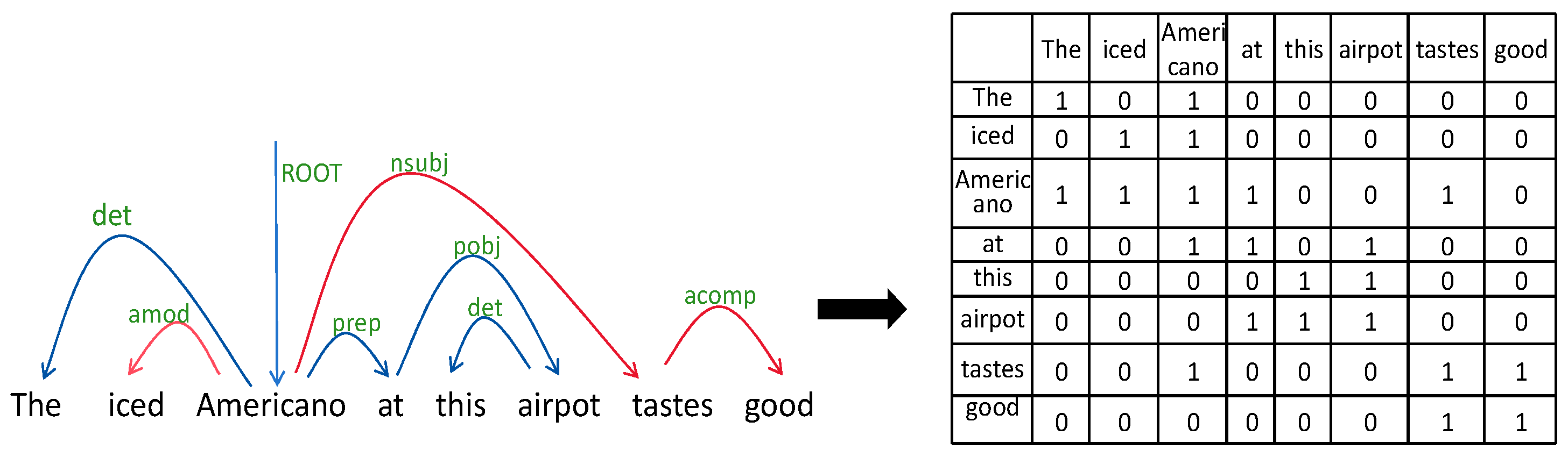
• The introduction of dependency parsing information in aspect-level sentiment analysis. By constructing an adjacency matrix of syntactic dependency relations, the model can more precisely capture the semantic correlations between different aspects in the text, thereby improving the precision and accuracy of sentiment analysis;
• To better integrate the features of both BERT and syntactic dependency relations, a multi-head attention mechanism is adopted. This mechanism considers different feature word vectors simultaneously, allowing the model to comprehend the semantic information of the text more comprehensively, thereby enhancing the performance;
• In order to bolster the robustness and generalizability of the model, an adversarial training mechanism is introduced. By applying small perturbations to the BERT embedding layer, FGM (fast gradient method) can make the model better resist attacks from adversarial samples, thus improving the model’s stability and reliability in real-world applications.

2. Related Work

2.1. Aspect-Level Sentiment Analysis

Aspect-level sentiment analysis is a vital task within sentiment analysis, concentrating on the sentiment polarity of particular aspect terms within a sentence. Traditional sentiment analysis methods often target entire documents or single sentences, whereas aspect-based sentiment analysis pays closer attention to more refined sentiment evaluations of specific entities. In past research, the use of traditional machine learning methods for sentiment classification has been a common practice. For instance, Kiritchenko et al. used SVM to detect aspect terms and sentiment in customer reviews [9]; Akhtar et al. employed SVM and CRF for Hindi sentiment classification with good results [10]; Patra et al. used CRF for aspect-level sentiment classification in the domains of Laptop and Restaurant datasets, providing valuable references for consumers and manufacturers [11]. However, these methods require manual feature selection and semantic information extraction, which can reduce the error of opinion word matching but still have limitations. For example, feature extraction from dataset texts requires a significant amount of labor, and the final sentiment analysis results are highly dependent on feature quality, but are incapable of modeling the dependencies between the provided aspect terms and their surrounding contexts.

Comparatively, deep neural networks possess more intricate model architectures and stronger feature extraction capabilities, eliminating the necessity for manual feature extraction, reducing labor costs. With the improvements in computer hardware performance and the widespread use of the Internet, deep neural networks are no longer limited by hardware computing power and data samples. In the realm of sequence models with a focus on attention, researchers have proposed a variety of methodologies. For example, Cheng et al. improved the feature extraction capacity of the Transformer bidirectional encoder through an extended context module and proposed a component focusing module to address the issue of average pooling [12]. Huang et al. proposed the AGSNP model, which combined attention mechanisms and achieved good results [13]. Ayetiran proposed a CNN and BiLSTM variant that combined high-level semantic feature extraction and sentiment polarity prediction [14]. In models focusing on syntactic information, Zeng et al. utilized affective knowledge to enhance word representations, forming a heterogeneous graph based on dependency trees, and designed a multi-level Semantic-HGCN to encode the graph for sentiment prediction [15]. Gu et al. proposed the EK-GCN model, which uses an external sentiment dictionary to assign sentiment scores to individual words within a sentence, constructing an emotional matrix to partially compensate for the shortcomings of the syntactic dependency tree [16]. In models focusing on contextual modeling, Xiao et al. proposed a novel GNN-based deep learning model, leveraging a POS-guided syntactic dependency graph for RGAT to eliminate noise and designing a syntactic distance attention-guided layer for DCGCN to extract semantic dependencies between contextual words [17]. Mewada et al. utilized affective knowledge to enhance word representations, forming a heterogeneous graph based on dependency trees, and then designing a multi-level Semantic-HGCN to encode the graph for sentiment prediction [18]. Xu et al. proposed a sentiment analysis model based on dynamic local context and dependency clusters, which dynamically captured the scope of local context and extracted semantic information, achieving good results [19]. Mao et al. proposed a multi-task learning approach, incorporating a novel gated bridging mechanism (GBM), which achieved superior performance in aspect-based sentiment analysis by effectively filtering irrelevant information and dynamically extracting features for each subtask using a weighted-sum pooling strategy [20].

2.2. Dependency Analysis

Dependency parsing, also known as dependency syntax analysis [21], aims to identify the interdependent relationships between words in a given text and find the corresponding dependent words (tail nodes) for each word (head node), which facilitates a deeper comprehension of the entire sentence’s meaning. This is also one of the more critical technologies in the field of NLP. The representation is through directed arrows from the central word to its dependent words, forming directed graphs. Dependency projection trees, and dependency trees are common ways to express dependency structures. Taking the sentence “The iced Americano at this airport tastes good” as an example, the expression of its dependency tree is as follows (Figure 1):

Dependency syntax analysis is typically represented as a tree structure, where the nodes of the tree represent words, the edges represent the dependency relationships between words, and the parent node of the tree indicates the governor. Some commonly used dependency relation labels, and their meanings in dependency syntax analysis, are presented in

Table 1. Partial dependency relationship labels and their meanings.

Labels	Meanings
ROOT	Root node
det	Dependency
amod	Adjectives
nsubj	Noun subjects
prep	Prepositional modifiers
pobj	Object of a preposition
acomp	Complement of an adjective

.

2.3. Adversarial Training

In the domain of computer vision (CV), it is essential to enhance the robustness of models through adversarial attacks and defenses. For instance, in autonomous driving systems, it is crucial to prevent models from misclassifying red lights as green due to random noise. Similarly, in natural language processing (NLP), adversarial training exists, primarily as a regularization technique aimed at enhancing model generalization.

In 2014, Szegedy et al. introduced the concept of adversarial examples, which is considered a pioneering work in the field [22]. For models processing text input data, the added perturbations can be categorized into two types: discrete, where perturbations are directly applied to the text; and continuous, where tiny perturbations are introduced into the word vector matrix. This paper employs the latter approach for adversarial training. Current popular adversarial training methods include the fast gradient sign method (FGSM) [23], fast gradient method (FGM), projected gradient descent (PGD) [24], free adversarial training (FreeAT) [25], and free large-batch (FreeLB) [26].

The core of adversarial training lies in constructing perturbations that enable the model to recognize diverse adversarial examples. Adversarial training algorithms first generate perturbations using adversarial attacks, then combine these perturbations with original samples to create adversarial examples. Subsequently, the model parameters are adjusted via backpropagation to minimize the loss function. This process can be defined as a max–min optimization problem, where the maximization problem involves finding perturbations that maximize the loss function for generating adversarial examples, while the minimization problem involves minimizing the loss function and updating model parameters, thereby endowing the model with robustness to adapt to such perturbations. Adversarial training can be uniformly represented as a min-max formula, as shown in the following equation:

$${min}_{\theta }{\mathbb{E}}_{\left(x,y\right)\sim \mathcal{D}}\left[{max}_{\mathsf{\Delta }x\in \Omega }L\left(x+\mathsf{\Delta }x,y;\theta \right)\right]$$

(1)

where $\mathcal{D}$ represents the dataset, $x$ represents the inputs, $y$ represents the labels, and $\theta$ is the model parameter that represents the parameter vector of the neural network, $L(x+\mathsf{\Delta }x,y;\theta )$ is a single sample of loss, $\mathsf{\Delta }x$ is the perturbation and $\Omega$ is the perturbation space. Then after the neural network function, the loss obtained by comparing with the label $y$, ${max}_{\mathsf{\Delta }x\in \Omega }L\left(\right)$ denotes the optimization objective.

2.4. Attention Mechanisms

In 2014, the Google Mind team’s paper brought attention mechanisms into the spotlight [27]. Initially introduced for image processing tasks, attention mechanisms have proven to be effective in other fields as well. Experimental validations have demonstrated the theoretical feasibility of attention mechanisms, and empirical results in the field of NLP have shown their efficacy in sentiment analysis tasks, highlighting their significant research value. This method is capable of effectively extracting key features, and as such, it is currently widely employed to enhance the performance of sentiment analysis models. The attention mechanism simulates the cognitive process of the human brain, quickly extracting valuable information from extensive text data and assigning higher weights to important information while assigning lower weights to other information.

Bahdanau et al. were the first to introduce attention mechanisms into machine translation based on the encoder–decoder model, successfully translating long sentences [28]. Despite potential issues with the encoding quality, attention mechanisms addressed this by allocating distinct weights to words in the encoding module based on their importance, leading to notable experimental results. The introduction of attention mechanisms has solved the problem of poor coding module quality for machine translation of long sentences, and this technology has been widely applied in the field of NLP, playing an especially important role in sentiment analysis tasks.

The unified computation method of the attention mechanism can be represented as follows:

$$Attention(Q,K,V)=softmax\left(Q{K}^T\right)V$$

(2)

In attention mechanisms, Q represents the query vector, K denotes the key vectors within a sentence, typically used for relevance calculations, and V represents the value vectors. Attention weights are obtained through a normalization method, which fundamentally maps the query vector to a series of relationships among key-value pairs. The structure can be visualized as follows (Figure 2):

3. Overall Model Design

This section begins with a description of the aspect-level sentiment analysis task, followed by the model structure.

3.1. Task Definition

The model input is the given text $W=\{w_1,w_2,\dots a,\dots o,\dots w_n\}$, where $a$ denotes an aspect word and $o$ denotes an opinion word, and the model outputs the sentiment polarity $y\in \{positive,negative,neutral\}$ corresponding to the aspect. Our model leverages the pre-trained language model BERT to generate and train word vectors.

3.2. Model Architecture

The model discussed in the paper comprises the following six main components: a text embedding layer, BERT encoding layer, syntactic dependency relation information layer, adversarial training layer, multi-head attention layer, and an output layer. The model’s overall structure is depicted in Figure 3.

3.2.1. Text Embedding Layer

For a sentence $W=\{w_1,w_2,\dots a,\dots o,\dots w_n\}$, use the pre-training model BERT to map each word onto an embedding vector $e_i\in R^{d\times 1}$, where d represents the dimension of the word vector:

$$W_{Bert}=Bert\left(W\right)$$

(3)

To fully leverage the power of BERT in model training, the text is formatted into the structure of “[CLS] + context + [SEP] + target + [SEP]”. In this format, “[CLS]” and “[SEP]” are special token markers utilized by BERT. “[CLS]” serves as a unique classification token marker that encapsulates classification-related information, while “[SEP]” functions as a separator to demarcate distinct sequences when multiple sequences are input. By adhering to the formatting requirements specified by BERT for text classification tasks, the effectiveness of BERT is maximized.

3.2.2. BERT Encoding Layer

The BERT encoder is constructed using Transformer blocks from the Transformer model [29]. For BERT-BASE, these blocks are employed in 12 layers, each consisting of 12 multi-head attention blocks. After passing through the BERT model, the output is a new sequence with the same length as $W_{Bert}$, represented as $H_{Bert}=\{h_{CLS},h_1,\dots ,h_{n-1}{,h}_{SEP},{h_a,h}_{SEP}\}$ as the representation of hidden vectors. Here, “$h_{CLS}$” is the hidden vector for the classification token, “$h_1$” to “$h_{n-1}$” are the hidden vectors for the context tokens, “$h_{SEP}$” represents the hidden vectors for the separator tokens, and “$h_a$” represents the hidden vectors for the aspect words.

3.2.3. Dependency Syntax Relation Information Layer

The text is simultaneously processed to establish syntactic dependency relations. In this paper, the StanfordCoreNLP tool is used to obtain the syntactic dependency tree of the text [30]. This is done by capturing the grammatical structure of sentences to extract dependency analysis; the output is a list containing multiple tuples. For example, in the sentence “The iced Americano at this airport tastes good”, the output is [(‘ROOT’,0,3), (‘det’,3,1), (‘amod’,3,2), (‘nsubj’,7,3), (‘prep’,4,3), (‘pobj’,6,4), (‘det’,6,5), (‘acomp’,8,7)]. In this sentence, there are a total of eight elements, so (‘amod’,3,2) indicates an adjective, where “Americano” depends on “iced”. Words in the sentence are encoded starting from 1 to the end of the sentence. The numbers in the tuple represent the positions of the words, and the numbers before and after represent the dependency relationship, where the first number is the head and the second number is the child, indicating that the latter depends on the former. Then, the dependencies are mapped onto a directed graph. The syntactic dependency tree can be conceptualized as graph G with n nodes, where the nodes correspond to the words in the sentence, and the edges represent the syntactic dependencies between words. The dependency parse tree of a sentence is represented as $G=\{V,A\}$, where V stands for all the nodes, which are the words $\{w_1,w_2,\dots a,\dots o,\dots w_n\}$; and $A\in {\mathbb{R}}^{n\times n}$ is the adjacency matrix, where $A_{ij}=1$ if there is a syntactic dependency between word $w_i$ and word $w_j$, and $A_{ij}=0$ otherwise. Each word in the sentence is adjacent to itself, which implies setting all diagonal elements of the adjacency matrix to 1 [31].

Here is how the syntactic dependency tree and its transformed adjacency matrix are depicted (Figure 4):

Next, the adjacency matrix is expanded into a one-dimensional vector and connected to the elements in the matrix row by row or column by column. The unfolded vector is used as an input for the next step of model processing. This converts the information of the adjacency matrix into a vector $V_{adj}$.

3.2.4. Adversarial Training Layer

The model uses the FGM (fast gradient method) for adversarial training on the BERT embedding layer vectors. FGM stands out from other methods due to its simplicity, ease of use, and computational efficiency. It generates adversarial samples with minimal parameter updates, making it practical for real-world applications with low computational costs, especially with large datasets and complex models. Despite potential variations in performance, FGM typically enhances model robustness against common adversarial attacks. Thus, FGM is a practical choice, particularly in resource-constrained scenarios or where rapid implementation is crucial. By performing gradient ascent based on the specific gradients, it aims to obtain better adversarial samples without significantly altering the distribution of the original samples, thereby allowing the model to adapt to such perturbations. Assuming that the embedding layer vectors $V=\{v_1,v_2,\dots ,v_n$} of the input text sequence are x, the perturbation on the embedding layer is as follows:

$$∆x=ϵ\frac{g}{\parallel g{\parallel }_2}$$

(4)

$$g={\nabla }_{x}L\left(x,y;\theta \right)$$

(5)

$$V_{adv}=V+∆x$$

(6)

After the adversarial training, the obtained feature vectors are denoted as $V_{adv}$.

3.2.5. Multi-Head Attention Mechanism Layer

After flattening the hidden features $H_{Bert}$ obtained from BERT’s output, we obtain $H_{Bert}^{\prime }$. Then, we concatenate it with the feature vector obtained after adversarial training to obtain the new hidden feature $Z=\left[H_{Bert}^{\prime }{,V}_{adj}\right]$. Z represents the input to the multi-head attention module. By utilizing three different weights $W_q$, $W_k$, $W_v$ in the attention layer, we can calculate the resulting vector $q$, $k$, $v$. The steps of the multi-head attention mechanism involve linearly transforming the query (Q), key (K), and value (V) through parameter matrices. Then, scaled dot-product operations are performed multiple times before concatenating the results. First, the score for each input feature is calculated: $score=k\times q$. Then, each score is normalized by dividing it by the square root of the dimension of the weight matrix $\sqrt{d_k}$. Next, the softmax function is applied to the normalized scores. Finally, the softmax result is multiplied by the value V. The formula is as follows:

$$a=softmax\left(\frac{Q{K}^T}{\sqrt{d_k}}\right)V$$

(7)

The multi-head attention mechanism assigns weighted attention scores to each word in the sentence using multiple attention mechanisms. By increasing the weight coefficients of important information, the model focuses more on words crucial for sentiment analysis, thus further enhancing the accuracy of sentiment analysis. The multi-head attention mechanism consists of multiple heads, each capable of generating different attention distributions, thereby addressing long-range dependencies. Built upon the attention mechanism, the multi-head attention mechanism significantly outperforms standard attention mechanisms, allowing for parallel processing of information in different positional and representational subspaces. With each set of attention projected into different spaces, and considering m as the number of attention heads, the calculation formula is as follows:

$${head}_i=a_i$$

(8)

$$e=MultiHead\left(Q,K,V\right)=Concat\left({head}_1,{head}_2,\dots ,{head}_m\right)W^O$$

(9)

Wherein, W^O represents the weight vector, which can be learned through the training process. The Concat function indicates the concatenation of the vectors after the attention computation, and head_i represents the i-th attention mechanism.

Finally, all encoding vectors are weighted and summed to obtain a comprehensive hidden expression e.

3.2.6. Output Layer

Considering that the adversarial perturbations in adversarial training are relatively small values, to prevent the word vectors from becoming too large, which could cause the tiny perturbations to lose their effectiveness, it is necessary to normalize the word vectors. Normalization ensures that the values of the word vectors remain within a reasonable range, allowing the model to be sensitive to the small adversarial perturbations. It is described as follows:

$$V_{\mathrm{a}\mathrm{d}\mathrm{v}}^{\prime }=\frac{V_{adv}-E\left(V_{adv}\right)}{\sqrt{Var\left(V_{adv}\right)}}$$

(10)

$$E\left(V_{adv}\right)=\sum _{i=1}^K{f}_i{V_{adv}}_i$$

(11)

$$Var\left(V_{adv}\right)=\sum _{i=1}^K{f}_i{\left({V_{adv}}_i-E\left(V_{adv}\right)\right)}^2$$

(12)

where $V_{adv}$ denotes the original word vector $V_{adv}^{\prime }$ denotes the normalized word vector and f_i denotes the frequency of the ith word in the training sample.

The fused features and adversarial features of the multi-head attention mechanism are, respectively, used as inputs to the Softmax classifier, after which the fused features of the multi-head attention mechanism and the real labels can be calculated as the classification loss Loss_mha, which is calculated by the following formula:

$$Los{s}_{mha}=\sum _{i=1}^N\left\{y_{i}log{\hat{y}}_i+\left(1-y_i\right)log\left(1-{\hat{y}}_i\right)\right\}$$

(13)

Wherein $y_i$ represents the true category, ${\hat{y}}_i$ represents the predicted category, and $N$ is the overall number of samples.

Subsequently, the adversarial features and the true labels are used as inputs to the classifier for calculating the adversarial training loss Loss_adv, with the following formula:

$$Los{s}_{adv}=-\frac{1}{N}\sum _{n=1}^N\mathit{log}p\left(y_n\mid x+\Delta x,\theta \right)$$

(14)

In this loss function, the variable is $x+\Delta x$, where $\Delta x$ represents the adversarial perturbation, $N$ is the overall number of samples, $y_n$ is the corresponding label, and $\theta$ is the model’s parameters that represents the parameter vector of the neural network. Therefore, the actual loss of the model is as follows:

$$Loss=Los{s}_{mha}+Los{s}_{adv}$$

(15)

Furthermore, the gradients of Loss_mha and Loss_adv with respect to the model parameters are computed first. Subsequently, these gradients, along with a predefined learning rate, are utilized to update the model parameters, aiming to progressively decrease the overall loss. Until it satisfies the predetermined maximum number of iterations, this iterative process continues. The generated adversarial training samples are used together with the original samples for model training. This approach can expand the dataset size and effectively enhance the model’s generalization performance and classification accuracy.

4. Experimental Analysis

4.1. Experimental Dataset and Experimental Environment

The model in this paper was mainly evaluated on the SemEval2014 Task4 public dataset, which consists of reviews from two domains, Laptops and Restaurants [32]; these datasets are partitioned into a training set and a test set. The aspect words and their corresponding sentiment polarity in the dataset have been labelled, where −1 represents negative, 0 represents neutral and 1 represents positive. The dataset’s fundamental statistics are provided in

Table 2. Basic statistical information of the dataset.

Datasets	Negative		Neutral		Postive
	Train	Test	Train	Test	Train	Test
Laptops	851	128	455	167	976	337
Restaurants	807	196	637	196	2164	727

.

Table 3. Configuration of experimental environment.

Experimental Environment Configuration Table	Configuration Information
Operating System CPU	AMD Ryzen 7 7735H with Radeon Graphics 3.20 GHz
Graphics card	NVIDIA GeForce RTX 4060
Deep Learning Framework	Pytorch
Development Environment	Pycharm

illustrates the pertinent configuration of the experimental environment in this paper.

4.2. Experimental Parameter Setting

The experiment used the pretrained language model BERT to generate word vectors. The generated word vectors have a dimension of 768, with a hidden-layer dimension of 300. The dropout rate is set to 0.1, and the learning rate is 2 × 10⁻⁵. The batch size for each input data is 32, and the optimizer used is Adam [33].

4.3. Evaluation Indicators

In the experiment, the evaluation metrics used were Accuracy and Macro-averaged F1 score [34,35]. Accuracy denotes the proportion of correctly classified positive and negative samples to the total number of samples. The F1 score is the harmonic mean of precision and recall, encompassing both precision and recall in the evaluation of the model. The macro-averaged F1 score is the average of the F1 scores for each category, which helps to avoid the issue of artificially high accuracy due to imbalanced data. The specific formulas are as follows:

$$Accurary=\frac{TP+TN}{TP+TN+FP+FN}$$

(16)

$$Precision=\frac{TP}{TP+FP}$$

(17)

$$Recall=\frac{TP}{TP+FP}$$

(18)

$$F1=\frac{2·Precision·Recall}{Precision+Recall}$$

(19)

$$MF1=\frac{1}{C}\sum _{k=1}^c{F1}_k$$

(20)

wherein TP represents the number of positive samples correctly predicted as positive, FN denotes the number of positive samples mistakenly predicted as negative, FP indicates the number of negative samples erroneously predicted as positive, and TN signifies the number of negative samples accurately predicted as negative. Precision and Recall denote the precision rate and recall rate, respectively, while C represents the number of sentiment categories.

To evaluate the significance of the improved results, we also added kappa consistency as a statistical test indicator. The Kappa coefficient, which is a statistical measure of consistency ranging between 0 and 1, is elaborated upon in

Table 4. Kappa coefficient table.

Coefficient	0.8–1.0	0.6–0.8	0.4–0.6	0.2–0.4	0–0.2
Level	Almost perfect	Substantial	Moderate	Fair	Slight

. A larger coefficient signifies greater precision in data classification. Its calculation formula is as follows:

$$K=\frac{P_o-P_e}{1-P_e}$$

(21)

$P_o$ represents the overall classification accuracy. The calculation formula for $P_e$ is as follows:

$$P_e=\frac{a_1\times b_1+a_2\times b_2+\cdot \cdot \cdot +a_k\times b_k}{n\times n}$$

(22)

$a_k$ represents the actual sample size of class k, $b_k$ represents the predicted sample size of class k, and the total sample size is n.

4.4. Comparative Experiments

The paper selected seven representative aspect-level sentiment analysis models to compare with the model provided in this paper, and their descriptions are as follows:

(1)

LSTM [36] is an aspect-level sentiment analysis model based on long short-term memory networks that uses a recurrent neural network structure for modeling and can capture temporal information in text. It performs sentiment classification by integrating the target word and context relationships through two LSTM layers that depend on the target;

(2)

TD-LSTM [37] utilizes LSTM to encode the contexts on both sides of the aspect term from different directions, and performs sentiment classification by concatenating the resulting feature representations;

(3)

MemNet [38] is a deep memory network model combined with an attention mechanism. By constructing multiple computational layers, each input layer adaptively selects deeper-level information and captures the correlation between each context word and the aspect via attention layers. The output of the final attention layer is utilized for sentiment polarity assessment;

(4)

IAN [39] utilizes two LSTM layers to acquire the hidden representations of the context and aspect terms. To precisely capture the semantic relationship between context words and the aspect term, an interactive attention mechanism is incorporated;

(5)

RAM [40] is a memory neural network model based on a recurrent attention mechanism that can effectively obtain the sentiment features between words that are farther apart;

(6)

AEN [41] utilizes an encoder with an attention mechanism to establish a sentiment analysis model between the context and its corresponding aspect term;

(7)

ASGCN [42] constructs a graph convolutional network on the sentence’s dependency tree to extract syntactic information. By integrating attention with masked aspect vectors and semantic information, it enhances sentiment classification performance;

(8)

GPT3+Prompt [43] is a language model that can be guided to perform aspect-level sentiment analysis tasks and generate relevant text by adding prompts.

Among all comparison models, the accuracy of the ASGCN model reached 75.55% and 80.77% on both datasets, respectively. This is because the ASGCN model constructs a graph convolutional network on the dependency tree of sentences, utilizing syntactic information to extract semantic relationships and improving the accuracy of sentiment classification.

The accuracy rates of LSTM and TD-LSTM on the two datasets reached 66.77% and 74.29%; and 67.71%, 75.36%, respectively. TD-LSTM improved the LSTM model, but because LSTM cannot reflect the interaction information between aspect words and text sentences, and LSTM processes sentences in the order of text sequences, the semantic information learned is not comprehensive enough, and too-long sentences can cause slow the gradient descent. The MemNet model’s attention mechanism for selecting deeper-level information may falter in filtering out noisy context words, potentially leading to reduced classification performance. Despite the IAN model’s precise capture of semantic relationships, it may face challenges with highly ambiguous context terms. The AEN model’s focus on context information might overlook subtle sentiment nuances. Lastly, the RAM model’s recurrent attention mechanism may introduce computational complexity and training instability. The above reasons have led to the poor performance of these models.

As indicated in

Table 5. Comparing the experimental results of the model on two publicly available datasets.

Comparative Models	Laptops			Restaurants
	Accurary	Macro-F1	Kappa	Accurary	Macro-F1	Kappa
LSTM	66.77	61.78	-	74.29	62.58	-
TD-LSTM	68.81	64.67	-	76.00	64.51	-
MemNet	70.64	65.17	-	79.61	69.64	-
IAN	71.20	66.69	-	76.86	66.71	-
RAM	72.32	67.90	0.6745	76.92	68.71	0.7148
AEN	73.69	68.59	0.6886	77.06	69.35	0.7262
ASGCN	75.55	71.05	0.6904	80.77	72.02	0.7377
GPT3 + Prompt	77.87	73.04	-	85.45	78.96	-
BAMD(Ours)	76.02	71.54	0.7171	83.04	76.61	0.7853

, the BAMD model surpasses other models in both Accuracy and Macro-F1 scores. On the two datasets, the accuracy rates of the BAMD model reached 76.02% and 83.04%, respectively. Our model offers several advantages over baseline models: first, by integrating dependency parsing information, we accurately capture semantic correlations between different aspects in the text. Second, employing a multi-head attention mechanism enables a comprehensive understanding of semantic information within the text. Lastly, the introduction of adversarial training enhances the model’s stability and reliability in real-world applications.

Although our model is only 1 to 2.5 percentage points less effective than the closed-source GPT3+Prompt, we acknowledge this difference. Our research suggests that, while our model may be lightweight, with fewer parameters and a smaller memory footprint, this lightweight nature makes it more feasible for deployment and operation in resource-constrained environments, with lower computational costs. While our model may slightly lag behind larger models in performance, its lightweight characteristics provide greater flexibility and feasibility for specific applications in certain scenarios. We will continue to strive for improvement and look forward to achieving better results in future research.

Moreover, it can be clearly seen from the chart that our model’s Kappa value is significantly better than the compared models. This indicates that our model can still maintain high classification consistency while considering randomness. The significance of this improvement is not only reflected in the Kappa value, but also in the robustness and generalization ability of the model on different datasets. Therefore, our model performs more reliably and stably in solving this classification task. The optimal performance metrics of each model on two datasets have been bolded in the table.

4.5. Ablation Experiment

To verify the importance of the three major modules designed in this paper, a series of ablation experiments were conducted.

For each ablation experiment, we can infer the importance of each component to model performance by the degree of degradation in the evaluation metrics:

The ablation experiment without Adversarial Training (w/o AT) exhibited a decrease in performance when compared to the original model. This is because adversarial training plays a crucial role in enhancing model robustness and generalization capabilities. Without adversarial training, the model is more susceptible to the influence of biased or noisy samples, leading to a decrease in performance. Therefore, adversarial training is vital for improving the robustness of the model.

Our model significantly outperformed the version without multi-head attention (w/o MHA). The multi-head attention mechanism aids in better integrating features from BERT and syntactic dependency relations, enhancing the model’s attention to different aspects of the text and its representational power. If the multi-head attention mechanism is removed, the model may not effectively capture sentiment information across different aspects, resulting in a decline in performance. It is evident that multi-head attention is important for enhancing the model’s representational capabilities.

The absence of syntactic dependency relations resulted in varying degrees of decline in both Accuracy and Macro-F1 scores. Syntactic dependency relations provide structural information between words in the text, which helps the model to better understand the semantic and logical relationships within sentences. If syntactic dependency relations are removed, the model may not effectively utilize the structural information of the sentence, leading to a decrease in performance. Therefore, syntactic dependency relations are important for enhancing the model’s semantic comprehension.

In summary, adversarial training, multi-head attention mechanism, and syntactic dependency relations each play a significant role in improving model performance. Together, they constitute the key components of the model proposed in this paper.

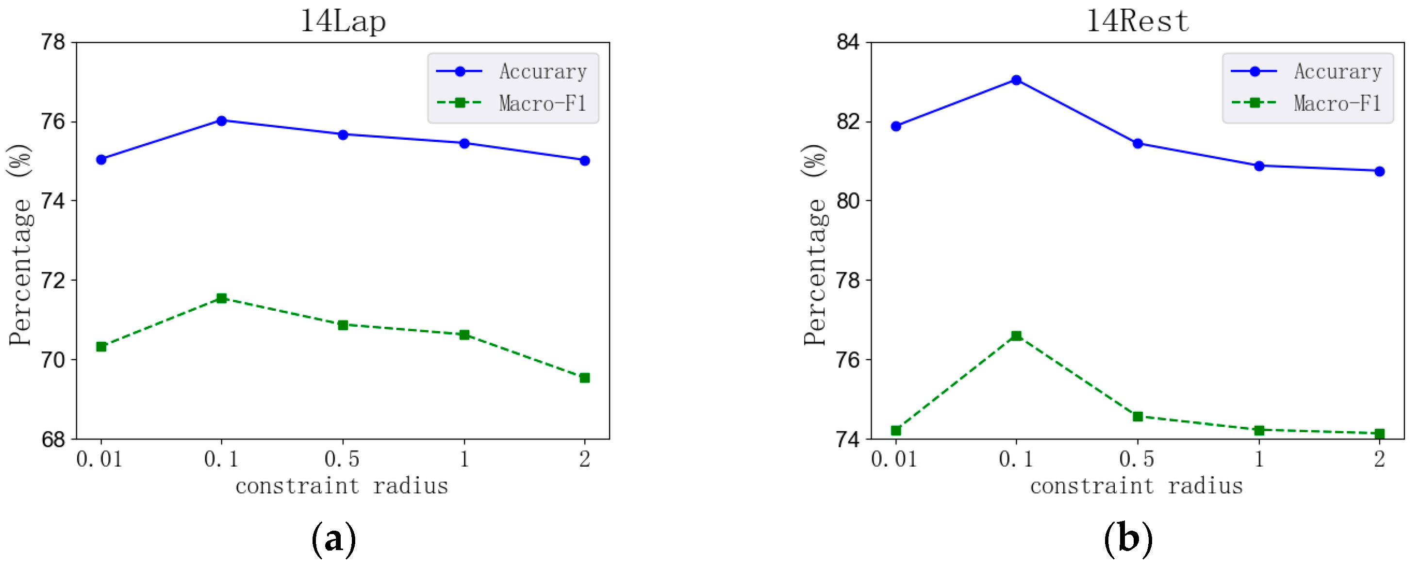
4.6. Analysis of Model Parameters

To investigate the impact of the constraint radius of the perturbation constraint space S, i.e., the value of ε, on model performance in adversarial training, this paper set ε values to 0.01, 0.1, 0.5, 1, and 2. The accuracy and MF1 scores were tested on both the 14Lap and 14Rest datasets (Figure 5). The experimental results, as shown in the figure below, indicate that introducing adversarial samples during the training stage can enhance the model’s resilience to attacks. The model performs optimally when the ε value is 0.1; however, when the ε value is too large, both the model’s accuracy and MF1 scores exhibit a downward trend. This phenomenon may be due to the larger perturbation values added, which resulted in significant differences between the generated adversarial samples and the original samples. Although they shared the same label, the model’s accuracy in identifying these adversarial samples decreased, subsequently leading to a decline in model performance.

4.7. Case Study

In order to reflect the effectiveness of the proposed approach, several specific examples were analyzed. Based on

Table 6. Results of ablation experiment.

Models	Laptops		Restaurants
	Accurary	Macro-F1	Accurary	Macro-F1
w/o DS	74.52	70.31	80.57	76.22
w/o AT	73.45	69.63	78.63	73.25
w/o MHA	73.58	69.97	79.78	74.56
BAMD	76.02	71.54	83.04	80.26

, we extracted the classification results of some typical examples for comparative analysis (

Table 7. Typical data experiment examples.

Num	Examples	TD-LSTM	ASGCN	BAMD	Label
1	The food is great but the service was dreadful!	Negative (×)	Positive (√)	Positive (√)	Positive
2	I’m delighted to return to the familiar embrace of Apple’s operating system.	Positive (√)	Negative (×)	Positive (√)	Positive
3	Did not enjoy the new Windows 8 and touchscreen functions.	Natural (×)	Positive (×)	Negative (√)	Negative

“√” in the table represents the model’s correct judgment of emotional polarity, while “×” represents the model’s incorrect judgment of emotional polarity.

).

For the first example sentence, due to the existence of two aspect terms, namely “food” and “service”, TD-LSTM focused on the opinion word “dreadful” related to “service”, considering it as the opinion word for the aspect term “food”, leading to an incorrect matching between aspect terms and opinion words, resulting in a negative sentiment judgment. In the second example sentence, the syntactic distance between “Apple’s operating system” and its opinion word “delighted” is too great. The aspect sentiment graph convolutional network (ASGCN) model failed to capture the relationship between them based on syntactic information, which resulted in an incorrect sentiment polarity judgment. The third example also contains two aspect terms, where TD-LSTM failed to accurately match aspect terms with opinion words, and ASGCN failed to capture the feature representation of the negation word “did not”. In contrast, BAMD combines both adversarial training and dependency syntax information, and thus can make accurate judgments.

5. Conclusions

This paper introduces an aspect-level sentiment analysis model that leverages adversarial training in conjunction with dependency syntax parsing. By employing BERT for word vector transformation, integrating feature extraction from syntactic dependency relations, and utilizing multi-head attention mechanisms along with adversarial training techniques, the proposed model is capable of predicting the sentiment polarity of specific aspects within sentences. On two public aspect-level sentiment analysis datasets, our model achieves higher accuracy and MF1 scores compared to the baseline models, validating the effectiveness of our approach. However, the model presented in this paper has certain limitations. For instance, the generated dependency syntax relations may contain data noise, and the influence of part-of-speech tags and other syntactic information on the task is not considered. The choice of the adversarial training method can be adjusted to optimize model performance for specific datasets. Future work will focus on further improving and enhancing the model to address these challenges. Specifically, we will explore methods to reduce data noise in generated dependency relations, incorporate part-of-speech tags and other syntactic information, and optimize adversarial training methods for specific datasets. These advancements aim to enhance the model’s performance and applicability in aspect-level sentiment analysis, thereby promoting its development and application in various domains.

References

1. Saberi, B.; Saad, S. Sentiment analysis or opinion mining: A review. Int. J. Adv. Sci. Eng. Inf. Technol. 2017, 7, 166–1666. [Google Scholar]
2. Medhat, W.; Hassan, A.; Korashy, H. Sentiment analysis algorithms and applications: A survey. Ain Shams Eng. J. 2014, 5, 1093–1113. [Google Scholar] [CrossRef]
3. Thet, T.T.; Na, J.C.; Khoo, C.S.G. Aspect-based sentiment analysis of movie reviews on discussion boards. J. Inf. Sci. 2010, 36, 823–848. [Google Scholar] [CrossRef]
4. Cortes, C.; Vapnik, V. Support-vector networks. Mach. Learn. 1995, 20, 273–297. [Google Scholar] [CrossRef]
5. Devlin, J.; Chang, M.W.; Lee, K.; Toutanova, K. Bert: Pre-training of deep bidirectional transformers for language understanding. arXiv 2018, arXiv:1810.04805. [Google Scholar]
6. Zhuang, L.; Wayne, L.; Ya, S.; Jun, Z. A robustly optimized BERT pre-training approach with post-training. In Proceedings of the 20th Chinese National Conference on Computational Linguistics, Huhhot, China, 13–15 August 2021; pp. 1218–1227. [Google Scholar]
7. Yang, Z.; Dai, Z.; Yang, Y.; Carbonell, J.; Salakhutdinov, R.R.; Le, Q.V. Xlnet: Generalized autoregressive pretraining for language understanding. Adv. Neural Inf. Process. Syst. 2019, 32, 5753–5763. [Google Scholar]
8. Mao, R.; Liu, Q.; He, K.; Li, W.; Cambria, E. The biases of pre-trained language models: An empirical study on prompt-based sentiment analysis and emotion detection. IEEE Trans. Affect. Comput. 2022, 14, 1743–1753. [Google Scholar] [CrossRef]
9. Kiritchenko, S.; Zhu, X.; Cherry, C.; Mohammad, S. Detecting aspects and sentiment in customer reviews. In Proceedings of the 8th International Workshop on Semantic Evaluation (SemEval), Dublin, Ireland, 23–24 August 2014; pp. 437–442. [Google Scholar]
10. Akhtar, M.S.; Ekbal, A.; Bhattacharyya, P. Aspect based sentiment analysis in Hindi: Resource creation and evaluation. In Proceedings of the Tenth International Conference on Language Resources and Evaluation (LREC’16), Portorož, Slovenia, 23–28 May 2016; pp. 2703–2709. [Google Scholar]
11. Patra, B.G.; Mandal, S.; Das, D.; Bandyopadhyay, S. Ju_cse: A conditional random field (crf) based approach to aspect based sentiment analysis. In Proceedings of the 8th International Workshop on Semantic Evaluation (SemEval 2014), Dublin, Ireland, 23–24 August 2014; pp. 370–374. [Google Scholar]
12. Cheng, L.C.; Chen, Y.L.; Liao, Y.Y. Aspect-based sentiment analysis with component focusing multi-head co-attention networks. Neurocomputing 2022, 489, 9–17. [Google Scholar] [CrossRef]
13. Huang, Y.; Peng, H.; Liu, Q.; Yang, Q.; Wang, J.; Orellana-Martín, D.; Pérez-Jiménez, M.J. Attention-enabled gated spiking neural P model for aspect-level sentiment classification. Neural Netw. 2023, 157, 437–443. [Google Scholar] [CrossRef]
14. Ayetiran, E.F. Attention-based aspect sentiment classification using enhanced learning through CNN-BiLSTM networks. Knowl.-Based Syst. 2022, 252, 109409. [Google Scholar] [CrossRef]
15. Zeng, Y.; Li, Z.; Chen, Z.; Ma, H. Aspect-level sentiment analysis based on semantic heterogeneous graph convolutional network. Front. Comput. Sci. 2023, 17, 176340. [Google Scholar] [CrossRef]
16. Gu, T.; Zhao, H.; He, Z.; Li, M.; Ying, D. Integrating external knowledge into aspect-based sentiment analysis using graph neural network. Knowl. Based Syst. 2023, 259, 110025. [Google Scholar] [CrossRef]
17. Xiao, L.; Xue, Y.; Wang, H.; Hu, X.; Gu, D.; Zhu, Y. Exploring fine-grained syntactic information for aspect-based sentiment classification with dual graph neural networks. Neurocomputing 2022, 471, 48–59. [Google Scholar] [CrossRef]
18. Mewada, A.; Dewang, R.K. SA-ASBA: A hybrid model for aspect-based sentiment analysis using synthetic attention in pre-trained language BERT model with extreme gradient boosting. J. Supercomput. 2023, 79, 5516–5551. [Google Scholar] [CrossRef]
19. Xu, M.; Zeng, B.; Yang, H.; Chi, J.; Chen, J.; Liu, H. Combining dynamic local context focus and dependency cluster attention for aspect-level sentiment classification. Neurocomputing 2022, 478, 49–69. [Google Scholar] [CrossRef]
20. Mao, R.; Li, X. Bridging towers of multi-task learning with a gating mechanism for aspect-based sentiment analysis and sequential metaphor identification. In Proceedings of the AAAI Conference on Artificial Intelligence, Virtually, 2–9 February 2021; Volume 35, pp. 13534–13542. [Google Scholar]
21. Nguyen, D.Q.; Verspoor, K. An improved neural network model for joint POS tagging and dependency parsing. arXiv 2018, arXiv:1807.03955. [Google Scholar]
22. Szegedy, C.; Zaremba, W.; Sutskever, I.; Bruna, J.; Erhan, D.; Goodfellow, I.; Fergus, R. Intriguing properties of neural networks. arXiv 2013, arXiv:1312.6199. [Google Scholar]
23. Goodfellow, I.J.; Shlens, J.; Szegedy, C. Explaining and harnessing adversarial examples. arXiv 2014, arXiv:1412.6572. [Google Scholar]
24. Madry, A.; Makelov, A.; Schmidt, L.; Tsipras, D.; Vladu, A. Towards deep learning models resistant to adversarial attacks. arXiv 2017, arXiv:1706.06083. [Google Scholar]
25. Shafahi, A.; Najibi, M.; Ghiasi, M.A.; Xu, Z.; Dickerson, J.; Studer, C.; Davis, L.S.; Taylor, G.; Goldstein, T. Adversarial training for free! Adv. Neural Inf. Process. Syst. 2019, 32, 3358–3369. [Google Scholar]
26. Zhu, C.; Cheng, Y.; Gan, Z.; Sun, S.; Goldstein, T.; Liu, J. Freelb: Enhanced adversarial training for natural language understanding. arXiv 2019, arXiv:arxiv:1909.11764. [Google Scholar]
27. Mnih, V.; Heess, N.; Graves, A. Recurrent models of visual attention. Adv. Neural Inf. Process. Syst. 2014, 27, 2204–2212. [Google Scholar]
28. Bahdanau, D.; Cho, K.; Bengio, Y. Neural machine translation by jointly learning to align and translate. arXiv 2014, arXiv:1409.0473. [Google Scholar]
29. Vaswani, A.; Shazeer, N.; Parmar, N.; Uszkoreit, J.; Jones, L.; Gomez, A.N.; Kaiser, Ł.; Polosukhin, I. Attention is all you need. Adv. Neural Inf. Process. Syst. 2017, 30, 5998–6008. [Google Scholar]
30. Manning, C.D.; Surdeanu, M.; Bauer, J.; Finkel, J.R.; Bethard, S.; McClosky, D. The Stanford CoreNLP natural language processing toolkit. In Proceedings of the 52nd Annual Meeting of the Association for Computational Linguistics: System Demonstrations, Baltimore, MD, USA, 23–24 June 2014; pp. 55–60. [Google Scholar]
31. Kipf, T.N.; Welling, M. Semi-supervised classification with graph convolutional networks. arXiv 2016, arXiv:1609.02907. [Google Scholar]
32. Kirange, D.K.; Deshmukh, R.R. Emotion classification of restaurant and laptop review dataset: Semeval 2014 task 4. Int. J. Comput. Appl. 2015, 113, 17–20. [Google Scholar]
33. Kingma, D.P.; Ba, J. Adam: A method for stochastic optimization. arXiv 2014, arXiv:1412.6980. [Google Scholar]
34. Chinchor, N.; Sundheim, B.M. MUC-5 evaluation metrics. In Proceedings of the Fifth Message Understanding Conference (MUC-5), Baltimore, MD, USA, 25–27 August 1993. [Google Scholar]
35. Yang, Y.; Liu, X. A re-examination of text categorization methods. In Proceedings of the 22nd Annual International ACM SIGIR Conference on Research and Development in Information Retrieval, Berkeley, CA, USA, 15–19 August 1999; pp. 42–49. [Google Scholar]
36. Greff, K.; Srivastava, R.K.; Koutník, J.; Steunebrink, B.R.; Schmidhuber, J. LSTM: A search space odyssey. IEEE Trans. Neural Netw. Learn. Syst. 2016, 28, 2222–2232. [Google Scholar] [CrossRef]
37. Tang, D.; Qin, B.; Feng, X.; Liu, T. Effective LSTMs for target-dependent sentiment classification. arXiv 2015, arXiv:1512.01100. [Google Scholar]
38. Tang, D.; Qin, B.; Liu, T. Aspect level sentiment classification with deep memory network. arXiv 2016, arXiv:1605.08900. [Google Scholar]
39. Ma, D.; Li, S.; Zhang, X.; Wang, H. Interactive attention networks for aspect-level sentiment classification. arXiv 2017, arXiv:1709.00893. [Google Scholar]
40. Chen, P.; Sun, Z.; Bing, L.; Yang, W. Recurrent attention network on memory for aspect sentiment analysis. In Proceedings of the 2017 Conference on Empirical Methods in Natural Language Processing, Copenhagen, Denmark, 7–11 September 2017; pp. 452–461. [Google Scholar]
41. Song, Y.; Wang, J.; Jiang, T.; Liu, Z.; Rao, Y. Attentional encoder network for targeted sentiment classification. arXiv 2019, arXiv:1902.09314. [Google Scholar]
42. Zhang, C.; Li, Q.; Song, D. Aspect-based sentiment classification with aspect-specific graph convolutional networks. arXiv 2019, arXiv:1909.03477. [Google Scholar]
43. Fei, H.; Li, B.; Liu, Q.; Bing, L.; Li, F.; Chua, T.S. Reasoning implicit sentiment with chain-of-thought prompting. arXiv 2023, arXiv:2305.11255. [Google Scholar]
Figure 1. Example diagram of dependency syntax tree.
Electronics 13 01993 g001
Figure 2. Attention mechanism structure.
Electronics 13 01993 g002
Figure 3. Model structure diagram.
Electronics 13 01993 g003
Figure 4. Syntactic dependency and adjacency matrix.
Electronics 13 01993 g004
Figure 5. (a) The accuracy of the model under different constraint radii (14Lap); and (b) the accuracy of the model under different constraint radii (14Rest).
Electronics 13 01993 g005