1. Introduction
Autosomal dominant polycystic kidney disease (ADPKD) is one of the most common hereditary renal disorders, characterized by the formation of multiple cysts in the kidneys, leading to a decrease in kidney function and eventual renal failure [
1,
2]. Patients typically experience end-stage renal failure due to the destruction of most nephrons after their 40s [
3]. While there are variations by country, ADPKD generally accounts for 5% to 10% of all end-stage renal disease cases.
Total kidney volume (TKV) indexed to patient height (htTKV) is an important imaging biomarker for assessing the severity of ADPKD [
4,
5,
6,
7,
8]. The Mayo classification uses htTKV at a single time point, adjusted for age and estimated kidney growth rate, to predict the time to requiring dialysis for patients with ADPKD with typical diffuse cystic kidney disease (Mayo class A) [
9]. The Food and Drug Administration (FDA)-approved indication for tolvaptan in ADPKD is to slow kidney function decline in adults at risk of rapidly progressing ADPKD [
10]. Magnetic resonance imaging (MRI) is recognized as an important tool for monitoring the progression of ADPKD, and the TKV and htTKV have been shown to predict renal function decline in ADPKD patients [
11]. The demand for MRI measurements of TKV has increased due to the importance of htTKV in determining eligibility for tolvaptan therapy and monitoring patients taking tolvaptan [
12].
When diagnosing lesions using MRI, multiple sequences can be utilized together. Two types of sequences, steady-state free precession (SSFP) and single-shot fast spin-echo (SSFSE), were utilized in this study. SSFP typically emphasizes contrast within substances like blood vessels, offering a high signal-to-noise ratio, but artifacts can arise around air or ferromagnetic materials. SSFSE enables rapid image acquisition with a high signal within substances, boasting fast scan speed and a strong signal. However, it may be limited in scenarios requiring low T2 contrast, sensitivity to motion, and high resolution or contrast. Although these sequences share similarities, their strengths differ, allowing for combined use in disease screening.
In a previous study, automated segmentation utilizing T2-weighted SSFSE and SSFP was confirmed. In this study, utilizing U-net on 213 MRI datasets from 129 individuals, Dice scores ranging from 0.94 to 0.98 and mean % differences ranging from 2.0% to 5.2% were achieved [
13].
However, in our study, we use a slightly different approach. We utilize a subtype of SSFP, called FIESTA (Fast Imaging Employing Steady-state Acquisition), from GE Healthcare, Chicago, IL, USA, along with SSFSE (Single Shot Fast Spin Echo) as training data. We use a learning method with a mixed dataset and then reinforcing learning through transfer learning. This allows us to create a segmentation model with higher accuracy using fewer data than conventional methods, thereby reducing the time required for image experts to perform segmentation and achieving more precise segmentation.
2. Materials and Methods
2.1. Dataset
This study was approved by the institutional review board (KUGH 2020-09-024-003). MRI data obtained from 85 patients with the assistance of Kosin University Gospel Hospital were utilized. Each patient contributed SSFSE and FIESTA MRI datasets. Each MRI image consisted of slices with dimensions of 512 × 512. The age range of the patients varied from a minimum of 20 to a maximum of 75 years, with an average age of 47.4 years, representing a diverse age group. The total number of images used for training amounted to 7158 for FIESTA and 7877 for SSFSE. Among these images, 80% were allocated to the training set, 10% to the validation set, and the remaining 10% to the test set. The exact information of the dataset is as given in
Table 1.
2.2. Data Preprocessing
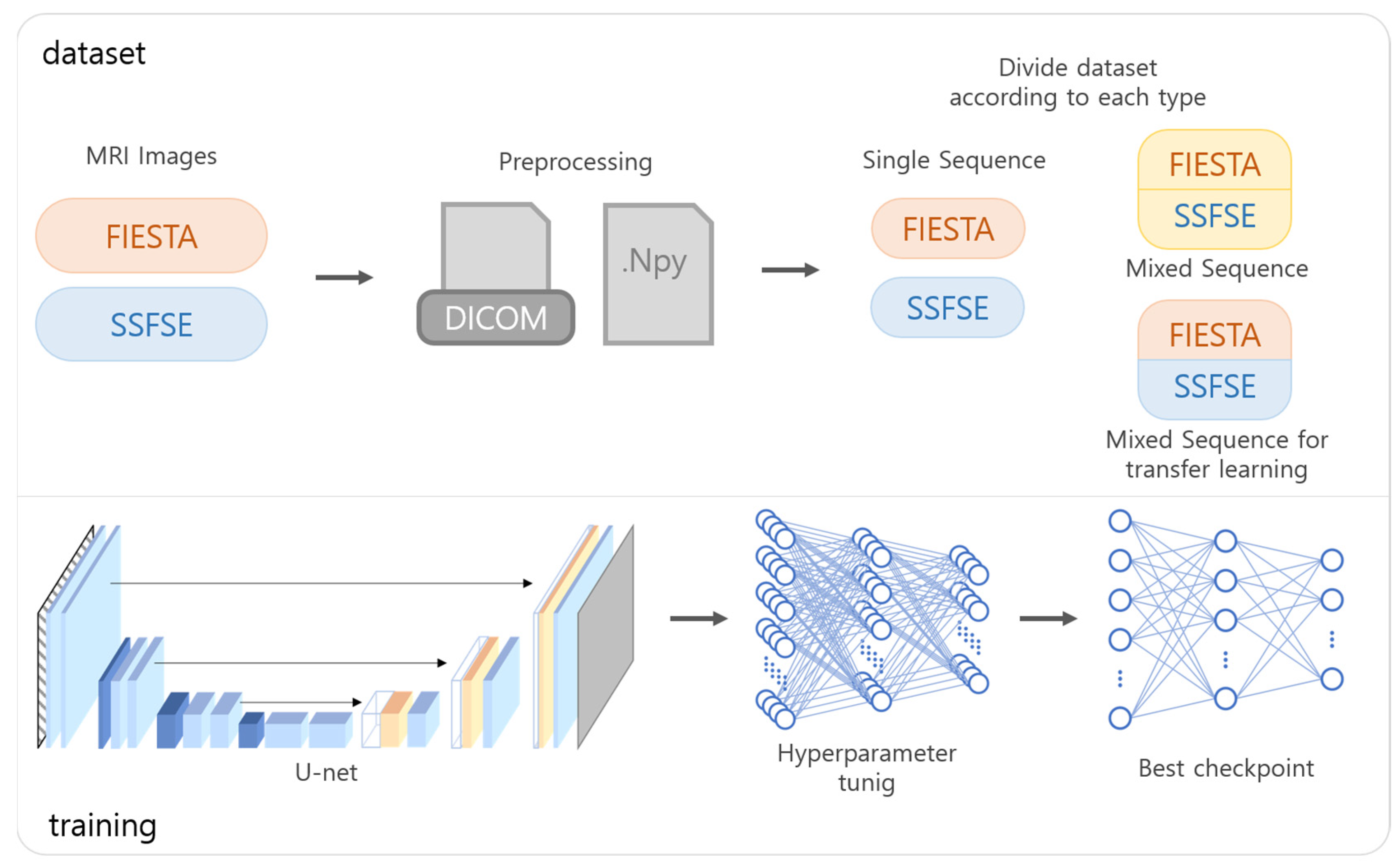
To prepare the data for training, DICOM files obtained through MRI were converted into NumPy format and transformed into image slices of size 512 × 512. The converted images were randomly shuffled and subsequently divided into respective datasets as shown in
Figure 1. The image slices used for training were individually normalized, and the ground truth labels were assigned based on data annotated by two abdominal radiologists (4 and 10 years of experience).
2.3. Model Training
The programming language used for training was Python (version 3.11), and the neural network was implemented using PyTorch (version 1.12.1). For the machine learning model focused on segmentation, a U-net model with four down-sampling and up-sampling layers was employed [
14,
15]. The model utilized a combination of the Dice coefficient loss function and the Adam optimizer. Training was conducted through six scenarios, distinguished by the MRI type: training exclusively on FIESTA, exclusively on SSFSE, training on both and applying to FIESTA, training on both and applying to SSFSE, fine-tuning after joint training to better fit FIESTA, and fine-tuning after joint training to better fit SSFSE. For the fifth and sixth scenarios, transfer learning was utilized. The data used in transfer learning were initially trained using subsets of each type’s dataset, followed by additional training using mixed data from diverse types.
2.4. Performance Evaluation
To compare the volume measurements of the kidneys obtained by imaging experts and those generated using artificial intelligence, the Dice coefficient was employed.
Additionally, a Bland–Altman analysis was conducted to evaluate the disparity between the TKV measured by experts and the predicted TKV [
16,
17]. The measurement of TKV involved calculating the total volume by utilizing the actual volume of voxels, determined by the pixel volume stored in the DICOM header of the MRI files.
3. Results
Dice Score and Volume Concordance
The Dice coefficients obtained using the six approaches that utilized images captured through the SSFE and FIESTA methods, as mentioned above, are presented in
Table 2. The Dice coefficient, volume concordance, and volume concordance standard deviation improve when the training method transitions from a single sequence dataset to a mixed dataset. Moreover, this improvement is even more pronounced during transfer learning compared to the mixed dataset used for training.
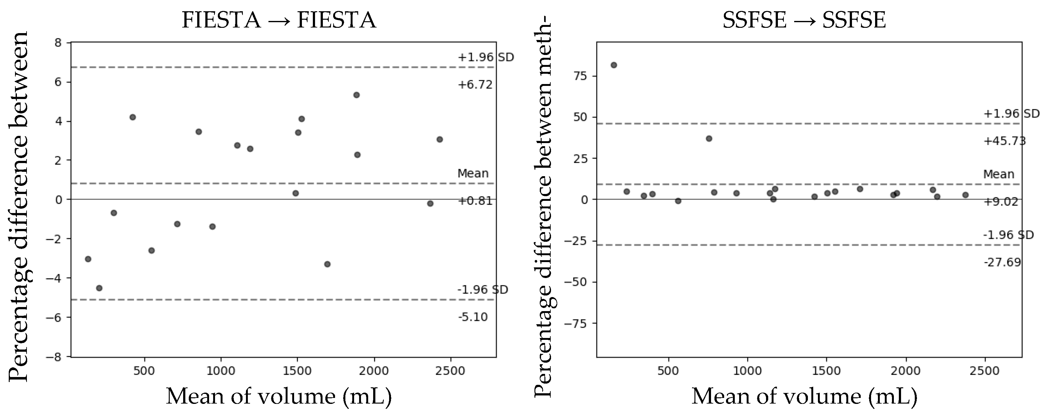
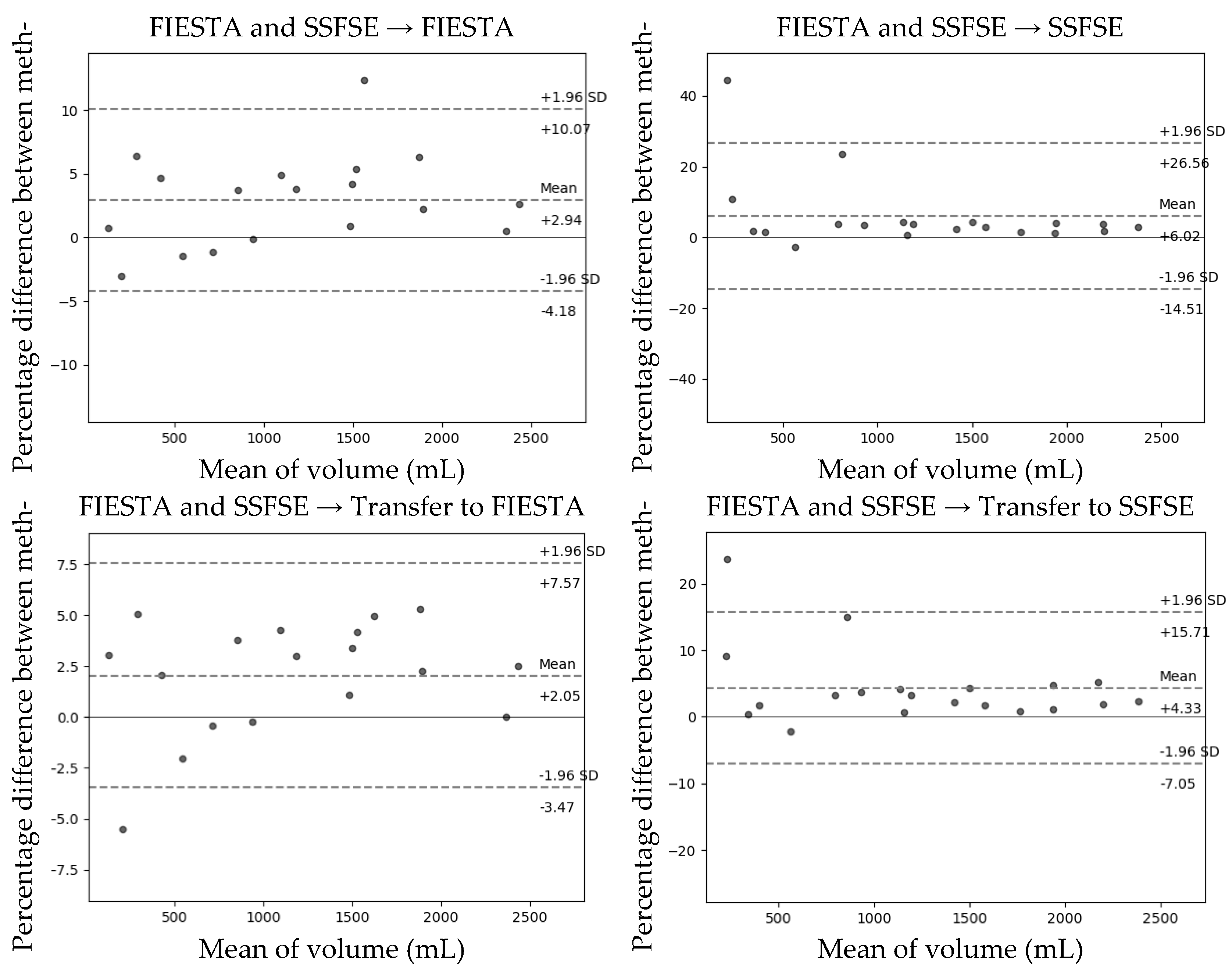
The Bland–Altman plot comparing the predicted total kidney volume (TKV) obtained through the developed model with the TKV measured by experts on the test set is shown in
Figure 2. In the transfer learning method, which is the learning group that showed the highest Dice coefficient as a result of Bland–Altman analysis, FIESTA had a mean difference of +2.05 when the Dice score was 0.951, and the 95% limit of agreement (LOA) interval was (−3.47, +7.57). In the case of SSFE, that had a mean difference of +4.33 when the Dice score was 0.952, and the 95% LOA interval was (−7.05, +15.71).
4. Discussion
Our study aimed to assess the performance of segmenting MRI images using the U-net model and enhancing accuracy by leveraging two different sequences. In the initial hypothesis, we anticipated that fine-tuning the model after joint training for both sequence types to optimize for each type would yield the best results.
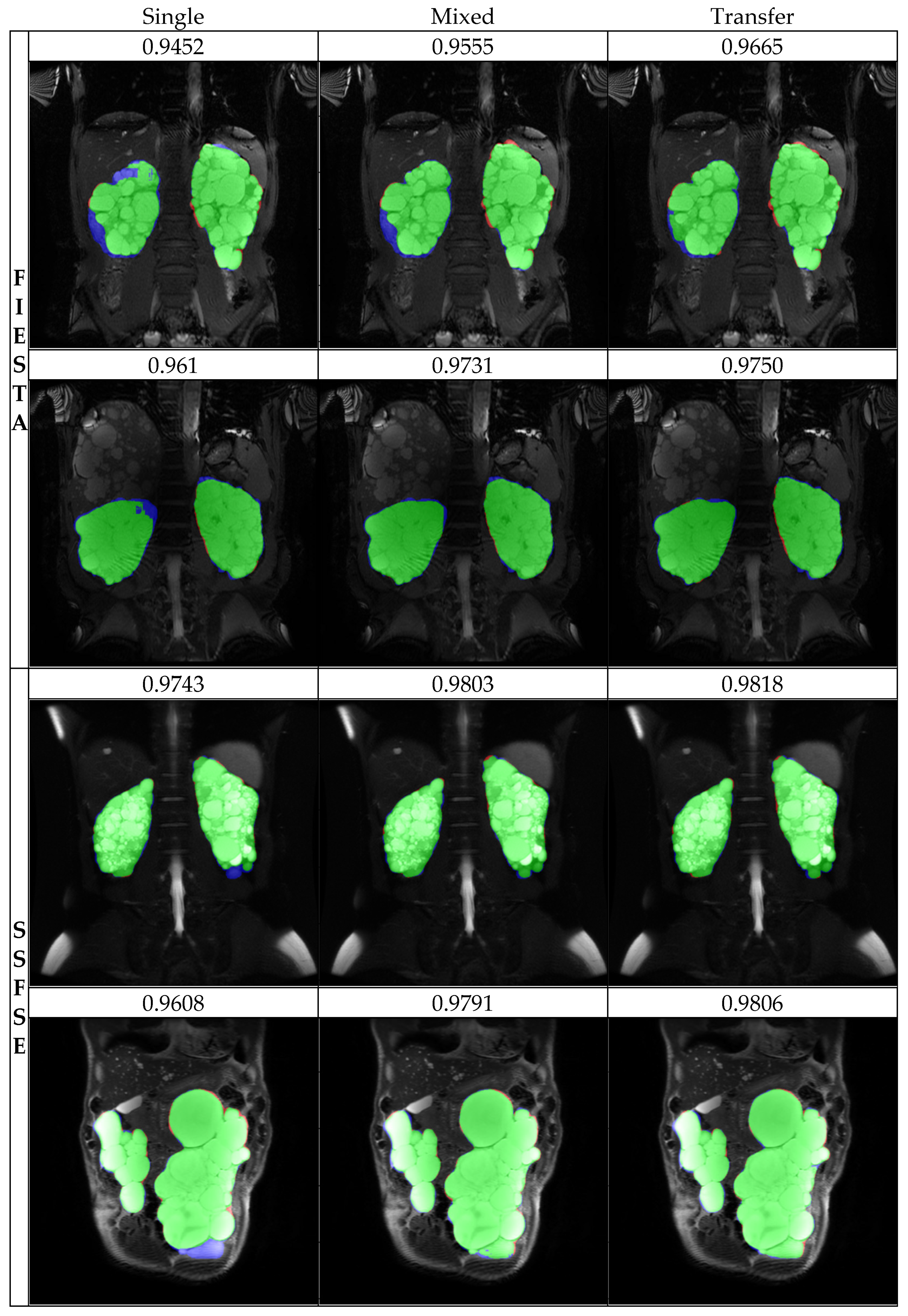
The results of the study showed that the accuracy of the model was highest when both FIESTA and SSFE sequences were trained together and then fine-tuned through transfer learning to better suit each sequence type. This outcome aligned with our expectations and resulted in the highest Dice coefficient scores and volume concordance for both FIESTA and SSFSE sequences. This not only resulted in a mere 2% increase in accuracy but also exhibited a significant difference in standard deviation. Specifically, in the SSFE, the standard deviation decreased from 9.09 to 4.54, nearly halving the value. Particularly noteworthy are the cases where severe errors occurred; the volume concordance improved from 18.8% in the single sequence setting to 76.3% after training on a mixed dataset followed by transfer learning. This demonstrates the capability of transfer learning with multi-sequences to rectify errors that could not be addressed through training on a single dataset. In the training results, as can be observed in
Figure 3, it is evident that the model’s predictions closely resemble the expert’s segmentation.
Among the images used for training, FIESTA exhibited artifacts with decreased center signals and Moiré effects, while SSFSE exhibited artifacts with decreased center signals. Particularly, within the dataset, the occurrence frequency of artifacts was higher in the case of FIESTA in
Figure 4. As a result, for SSFSE, there were fewer cases with artifacts in the training dataset, causing significantly lower Dice scores in predictions when artifacts were present during testing. However, for FIESTA, cases with artifacts were sufficiently represented in the training dataset, resulting in relatively higher Dice scores even in cases with artifacts during testing.
Furthermore, when both SSFSE and FIESTA were jointly trained and fine-tuned to be more suitable for SSFSE, the Dice scores notably improved. This demonstrates that artifacts obtained from the two distinct image acquisition sequences, FIESTA and SSFSE, can complement each other, enhancing the accuracy of training.
5. Conclusions
Our study demonstrated that by utilizing U-net, we can achieve kidney volume segmentation with a high level of accuracy comparable to that of experts. Moreover, our research revealed that the accuracy of the two distinct MRI acquisition sequences, SSFE and FIESTA, can influence each other’s performance. However, for cases with specific errors, similar error cases need to be adequately represented in the training set to further enhance accuracy during testing. To further enhance the model’s accuracy in achieving precise segmentation, additional research using larger and more diverse datasets is necessary.
Author Contributions
Conceptualization, Y.-C.A. and J.-G.P.; methodology, M.-S.K.; software, M.-S.K.; validation, J.-G.P. and M.-S.K.; formal analysis, M.-S.K. and J.-G.P.; investigation, J.-G.P. and M.-S.K.; resources, Y.-S.J.; data curation, Y.-S.J.; writing—original draft preparation, M.-S.K.; writing—review and editing, Y.-C.A.; visualization, M.-S.K.; supervision, Y.-C.A.; project administration, Y.-C.A.; funding acquisition, Y.-C.A. All authors have read and agreed to the published version of the manuscript.
Funding
This research was supported by grants from the Korea Institute of Marine Science and Technology Promotion (KIMST) through funding provided by the Ministry of Oceans and Fisheries (Grant No. 20210695).
Data Availability Statement
The data is unavailable due to privacy or ethical restrictions.
Conflicts of Interest
The authors declare no conflict of interest.
References
- Cornec-Le Gall, E.; Alam, A.; Perrone, R.D. Autosomal dominant polycystic kidney disease. Lancet 2019, 393, 919–935. [Google Scholar] [CrossRef] [PubMed]
- Grantham, J.J. The etiology, pathogenesis, and treatment of autosomal dominant polycystic kidney disease: Recent advances. Am. J. Kidney Dis. 1996, 28, 788–803. [Google Scholar] [CrossRef] [PubMed]
- Chapman, A.B.; Devuyst, O.; Eckardt, K.U.; Gansevoort, R.T.; Harris, T.; Horie, S.; Kasiske, B.L.; Odland, D.; Pei, Y.; Perrone, R.D.; et al. Autosomal-dominant polycystic kidney disease (ADPKD): Executive summary from a Kidney Disease: Improving Global Outcomes (KDIGO) Controversies Conference. Kidney Int. 2015, 88, 17–27. [Google Scholar] [CrossRef] [PubMed]
- Sedman, A.; Bell, P.; Manco–Johnson, M.; Schrier, R.; Warady, B.A.; Heard, E.O.; Butler–Simon, N.; Gabow, P. Autosomal dominant polycystic kidney disease in childhood: A longitudinal study. Kidney Int. 1987, 31, 1000–1005. [Google Scholar] [CrossRef] [PubMed]
- Grantham, J.J.; Torres, V.E.; Chapman, A.B.; Guay-Woodford, L.M.; Bae, K.T.; King Jr, B.F.; Wetzel, L.H.; Baumgarten, D.A.; Kenney, P.J.; Harris, P.C. Volume progression in polycystic kidney disease. N. Engl. J. Med. 2006, 354, 2122–2130. [Google Scholar] [CrossRef] [PubMed]
- Chapman, A.B.; Wei, W. Imaging approaches to patients with polycystic kidney disease. In Proceedings of the Seminars in Nephrology; WB Saunders: Philadelphia, PA, USA, 2011; pp. 237–244. [Google Scholar]
- Alam, A.; Dahl, N.K.; Lipschutz, J.H.; Rossetti, S.; Smith, P.; Sapir, D.; Weinstein, J.; McFarlane, P.; Bichet, D.G. Total kidney volume in autosomal dominant polycystic kidney disease: A biomarker of disease progression and therapeutic efficacy. Am. J. Kidney Dis. 2015, 66, 564–576. [Google Scholar] [CrossRef]
- Grantham, J.J.; Torres, V.E. The importance of total kidney volume in evaluating progression of polycystic kidney disease. Nat. Rev. Nephrol. 2016, 12, 667–677. [Google Scholar] [CrossRef] [PubMed]
- Alan, S.; Shen, C.; Landsittel, D.P.; Harris, P.C.; Torres, V.E.; Mrug, M.; Bae, K.T.; Grantham, J.J.; Rahbari-Oskoui, F.F.; Flessner, M.F. Baseline total kidney volume and the rate of kidney growth are associated with chronic kidney disease progression in Autosomal Dominant Polycystic Kidney Disease. Kidney Int. 2018, 93, 691–699. [Google Scholar]
- US Food and Drug Administration. Available online: https://www.accessdata.fda.gov/drugsatfda_docs/nda/2018/204441Orig1s000Approv.pdf (accessed on 6 September 2018).
- Irazabal, M.V.; Rangel, L.J.; Bergstralh, E.J.; Osborn, S.L.; Harmon, A.J.; Sundsbak, J.L.; Bae, K.T.; Chapman, A.B.; Grantham, J.J.; Mrug, M. Imaging classification of autosomal dominant polycystic kidney disease: A simple model for selecting patients for clinical trials. J. Am. Soc. Nephrol. 2015, 26, 160–172. [Google Scholar] [CrossRef] [PubMed]
- Torres, V.E.; Chapman, A.B.; Devuyst, O.; Gansevoort, R.T.; Grantham, J.J.; Higashihara, E.; Perrone, R.D.; Krasa, H.B.; Ouyang, J.; Czerwiec, F.S. Tolvaptan in patients with autosomal dominant polycystic kidney disease. N. Engl. J. Med. 2012, 367, 2407–2418. [Google Scholar] [CrossRef] [PubMed]
- Goel, A.; Shih, G.; Riyahi, S.; Jeph, S.; Dev, H.; Hu, R.; Romano, D.; Teichman, K.; Blumenfeld, J.D.; Barash, I.; et al. Deployed Deep Learning Kidney Segmentation for Polycystic Kidney Disease MRI. Radiol. Artif. Intell. 2022, 4, e210205. [Google Scholar] [CrossRef]
- Fatemeh, Z.; Nicola, S.; Satheesh, K.; Eranga, U. Ensemble U-net-based method for fully automated detection and segmentation of renal masses on computed tomography images. Med. Phys. 2020, 47, 4032–4044. [Google Scholar] [CrossRef] [PubMed]
- Ronneberger, O.; Fischer, P.; Brox, T. U-net: Convolutional networks for biomedical image segmentation. In Proceedings of the Medical Image Computing and Computer-Assisted Intervention–MICCAI 2015: 18th International Conference, Munich, Germany, 5–9 October 2015; Proceedings, Part III 18, 2015. pp. 234–241. [Google Scholar]
- Altman, D.G.; Bland, J.M. Measurement in medicine: The analysis of method comparison studies. J. R. Stat. Soc. Ser. D Stat. 1983, 32, 307–317. [Google Scholar] [CrossRef]
- Myles, P.S.; Cui, J. Using the Bland-Altman method to measure agreement with repeated measures. Br. J. Anaesth. 2007, 99, 309–311. [Google Scholar] [CrossRef] [PubMed]
| Disclaimer/Publisher’s Note: The statements, opinions and data contained in all publications are solely those of the individual author(s) and contributor(s) and not of MDPI and/or the editor(s). MDPI and/or the editor(s) disclaim responsibility for any injury to people or property resulting from any ideas, methods, instructions or products referred to in the content. |
© 2024 by the authors. Licensee MDPI, Basel, Switzerland. This article is an open access article distributed under the terms and conditions of the Creative Commons Attribution (CC BY) license (https://creativecommons.org/licenses/by/4.0/).


