Abstract
This paper presents a computer vision-based standalone decision-aid landing system for light fixed-wing aircraft, aiming to enhance safety during emergency landings. Current landing assistance systems in airports, such as Instrument Landing Systems (ILSs) and Precision Approach Path Indicators (PAPIs), often rely on costly and location-specific ground equipment, limiting their utility for low-payload light aircraft. Especially in emergency conditions, the pilot may be forced to land on an arbitrary runway where the road flatness and glide angle cannot be ensured. To address these issues, a stereo vision-based auxiliary landing system is proposed, which is capable of estimating an appropriate glide slope based on the terrain, to assist pilots in safe landing decision-making. Moreover, in real-world scenarios, challenges with visual-based methods arise when attempting emergency landings on complex terrains with diverse objects, such as roads and buildings. This study solves this problem by employing the Gaussian Mixture Model (GMM) to segment the color image and extract ground points, while the iterative weighted plane fitting (IWPF) algorithm is introduced to mitigate the interference of outlier feature points, reaching a highly robust plane normal estimation. With the aid of the proposed system, the pilot is able to evaluate the landing glide angle/speed with respect to the uneven terrain. Simulation results demonstrate that the proposed system can successfully achieve landing guidance in unknown environments by providing glide angle estimations with an average error of less than 1 degree.
1. Introduction
1.1. Research Purpose and Contributions
The process of aircraft landing is inherently complex and high-risk, influenced by various dynamic factors such as weather conditions, surroundings, pilot experience, and ground equipment reliability. Statistical data [1] reveal that landing-related accidents account for up to 56% of all flight accidents. Despite the presence of advanced instruments in modern airports, landing failures still occur with notable frequency. In addition, owing to cost constraints and limited flight capacity, some light aircraft operate without the aid of additional advanced navigation systems, as illustrated in Figure 1a,b. During emergency situations like engine failure or flight termination, pilots may be required to execute landings without the aid of third-party ground equipment, thus escalating the risk of accidents. For instance, Figure 1a,b showcase a light aircraft landing on a highway, where the pilot heavily relied on vision to perceive the surroundings.

Figure 1.
Real-world light aircraft emergency landing cases: (a–d) images from [2,3,4,5].
In the past, manual landings were commonplace before the advent of modern airport facilities, leading to accidents resulting from pilot error or misjudgment [6]. Furthermore, the high pilot workload during landing can lead to distractions and inadequate processing of visual information, potentially leading to incorrect gliding angles and descending speeds, with the possibility of severe consequences such as fuselage crashes or wing damage. In contrast to manual landings, modern airports offer advanced ground equipment, like the Instrument Landing System (ILS) and Precision Approach Path Indicator (PAPI), to assist pilots in landing safely, even in challenging conditions [7]. Nevertheless, this equipment is not available on every runway due to its high costs and maintenance fees [8]. Also, the installation of the associated instruments required by the ILS may be not applicable to light aircraft. Consequently, the development of an onboard standalone environmental perception system becomes a critical challenge.
As a result, the objective of this study is to propose a terrain-awareness landing assistance system for fixed-wing aircraft. The main contributions are summarized as follows: (1) The proposed system offers 6 degrees of freedom (6DoF) standalone localization and guidance, enabling safe landings on diverse terrain types. (2) The developed perception algorithm is able to mitigate the interference of inappropriate glide slope and descending rates by providing the estimated ground slope and aircraft localization. (3) Additionally, the system design prioritizes cost-effectiveness and lightweight features to facilitate installation on small aircraft and UAVs. (4) Moreover, operating as a self-contained system, the developed system eliminates dependency on third-party equipment, thereby enabling deployment in light fixed-wing aircraft. (5) Lastly, the developed auxiliary landing assistance system is capable of providing real-time environmental and risk awareness during landing. To the best of our knowledge, there are few works that focus on developing a low-cost onboard environmental awareness landing auxiliary system for fixed-wing light aircraft. Thus, this paper aims to develop an original framework that helps pilots perceive the landing environment in a more intuitive way. In detail, the proposed system estimates the current aircraft pose and the local ground normal vector, as illustrated in Figure 2a. By aligning the z-axis of the aircraft’s body frame with the ground normal, a proper landing attitude can be guaranteed. Additionally, real-time status showing whether the aircraft is too high, too low, or not aligned with the center is provided by the system, as shown in Figure 2b, enabling the pilot to prevent heavy landings.
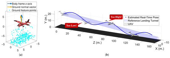
Figure 2.
Schematic of system features: (a) ground normal vector estimation (b) height alarm system.
To realize the aforementioned achievements, Simultaneous Localization and Mapping (SLAM)-related technology is applied. The stereo vision-based SLAM is independent of external ground equipment, making it an ideal choice for developing a lightweight and standalone aircraft landing auxiliary system. The authors of [9] indicated that SLAM has been the preferred choice in recent years for perceiving the environment and estimating ego-motion. In addition, the common sensors used in SLAM include monocular cameras, stereo cameras, RGB-D cameras, and LiDAR. Among these sensors, the stereo camera [10] stands out for its capability for large-scale usage, lightweight nature, and low-cost features, which fulfill our system requirements and the properties of the landing scenario. Also, compared to a monocular camera, it does not suffer from scale ambiguity and can use disparity to recover the depth information of pixels.
Among the state-of-the-art stereo V-SLAM frameworks, comparisons presented in [11,12] showed that ORB-SLAM2 achieves the best performance. Considering the exceptional results and its real-time efficiency, ORB-SLAM2 is selected as the base method in our system. It is responsible for estimating the localization of the aircraft and producing the 3D feature map.
1.2. Review and Examination of ORB-SLAM2
As illustrated in Figure 3, ORB-SLAM is a renowned SLAM framework compatible with monocular, stereo, and RGB-D cameras. In the case of a rectified stereo system, the ORB-SLAM2 pipeline begins by establishing 3D map points from a stereo image pair. To achieve this, the 256-bit ORB features [13] are extracted and matched [14] between the left and right images, utilizing either the brute-force method or FLANN [15]. Both stereo and monocular feature points are then fed into the three main parallel threads of ORB-SLAM2: tracking, local mapping, and loop-closing.

Figure 3.
Revised ORB-SLAM2 framework for landing scenarios [16]. The blocks inside the red box would be disabled in this work considering the property of landing.
The tracking thread assumes a constant velocity model and preliminarily calculates the pose of the current frame. Subsequently, it performs a motion-only bundle adjustment (BA) to further refine the pose. In case of tracking loss, a relocalization process is carried out. The optimization problem is divided into steps to ensure improved convergence results. Following keyframe selection, the local mapping thread is activated to filter keyframes and optimize the poses and map points of historical keyframes, which involves creating and culling map points, as well as local BA. The third thread in ORB-SLAM2 is loop-closing, which continuously performs place recognition by checking the covisibility graph. Upon detecting a closed loop, pose graph optimization corrects previously estimated poses, followed by full BA to ensure global consistency. This approach effectively addresses accumulated errors in exploration. With well-formulated strategies, ORB-SLAM2 operates these three threads simultaneously and successfully estimates poses and observed points, even for relatively large scales.
Most applications of ORB-SLAM2 primarily focus on autonomous vehicles navigating urban, highway, and indoor environments [11,12]. In these scenarios, the system encounters complex image features due to the presence of various objects, lighting conditions, and shadows. However, the landing scenario, crucial for ensuring high flight safety standards, differs significantly, as it involves a relatively uniform and monotonous visual environment, with few random objects near the runway.
In such monotonous scenarios, a significant proportion of image features exhibit high similarity to each other, leading to potential mismatches and reduced localization accuracy. Moreover, previous research [14] suggested a method of dividing the image into smaller grids and adjusting the ORB feature threshold until at least five feature points are extracted from each grid. However, this method may not be suitable for simple landing scenarios where the runway lacks complex features.
During the landing phase, the pilot aligns the center of the runway with the nose direction, leading to a fixed glide angle and constrained view from the aircraft. This constraint can cause the extracted ORB features to remain largely unchanged if there are insufficient nearby feature points observed, resulting in underestimated forward trajectory estimation.
Meanwhile, since a landing scenario does not involve revisiting previously encountered scenes, the loop-closing thread in ORB-SLAM2 should not detect loop closures. However, due to the high similarity among ORB features in this context, there is a risk of improperly triggering the loop-closing thread if the associated criteria are not well defined. Consequently, to prevent false detection, the loop-closing thread is disabled in this work, as highlighted by the red part in Figure 3.
These unique characteristics of the landing scenario, including uniform image features, limited forward view variation, and the absence of recurring scenes, present specific challenges for the ORB-SLAM2 framework. Overcoming these challenges is crucial to ensuring accurate localization and mapping during landing operations.
Additionally, in the landing process, the main focus is on maintaining the correct glide slope and descent speed to ensure a smooth touchdown and avoid excessive rolling or heavy landings. Thus, precise measurement of the historical trajectory becomes less critical. Instead, real-time acquisition of current localization along the vertical (z-axis) and lateral (y-axis) axes, namely and in the translation vector , is much more important. Additionally, accurately estimating the rotation matrix is essential for maintaining a consistent glide slope for the aircraft.
2. GMM-Based Landing Area Extraction
Previous research [17] evaluated the performance of ORB-SLAM2 in scenes with different image feature complexities, showing that while ORB-SLAM2 offers 6DoF localization for aircraft, the feature maps generated under complex scenes include a significant number of non-ground points, increasing the difficulty of estimating the ground slope. Additionally, the accuracy of localization shows a decline in monotonous scenes, as discussed in the previous section. These phenomena both present a challenge when calculating the glide slope. In this section, an optimized Gaussian Mixture Model (GMM)-based ground extraction algorithm is presented. The concept of image segmentation using the GMM is first discussed, followed by the methods for enhancing the efficiency and robustness of the color image segmentation process. Additionally, the integration issues between our proposed method and ORB-SLAM2 are addressed, along with corresponding solutions.
The GMM is a widely used data analysis method capable of classifying data points into different groups based on their distribution. In various research fields, image segmentation is a crucial step in extracting specific objects of interest from the overall view. For instance, in autonomous driving, lane line detection is a fundamental problem for guidance design. Previous research papers, such as [18,19], employed the GMM as the primary technique for analyzing images and extracting lane curves for car guidance laws. The robustness of the GMM’s segmentation results can be ensured with a well-designed image-processing pipeline. Another study [20] provided detailed guidance on formulating the lane line extraction method based on the GMM and integrated the estimation results with Hough lines to achieve a high level of robustness in challenging driving scenes. Additionally, the GMM has shown potential in object tracking, as demonstrated in [21,22]. A 1D GMM fitting algorithm can be derived through Maximum Likelihood Estimation (MLE), and its pseudo-code is listed in Algorithm 1.
| Algorithm 1 The 1D GMM fitting algorithm. |
| Input: : initial guess of GMM parameters; K: total number of clusters |
| : tolerance for iteration; : maximum iteration times; |
| Output: |
| 1: while Iteration time do |
| 2: update |
| 3: update |
| 4: update |
| 5: update |
| 6: if the update amount < then |
| 7: break |
| 8: end if |
| 9: end while |
2.1. Image Segmentation in CIE-Lab Color Space
CIE-Lab represents colors by combining lightness (L*) with two color component axes, a* and b*, which correspond to the red-green and blue-yellow color dimensions, respectively. To segment color images, the two channels describing color information are used to perform GMM fitting.
Algorithm 1 summarizes the input for the GMM, which includes the data, initial guesses of the Gaussian parameters , and desired total number of clusters, K. These parameters play a crucial role in the convergence speed and accuracy of data fitting, similar to other fitting algorithms. Therefore, GMM color image segmentation can be optimized through three aspects: (1) reducing data size, (2) determining the best input parameters for the GMM, and (3) self-adjusting the GMM cluster number K by considering the mission properties. To demonstrate the effectiveness of these methods, the finalized pipeline and example results using both simple and complex landing scenes are presented.
First, to simplify the evaluation of the GMM’s time cost, a 1D data sequence is used to simulate a landing procedure, originally sized at 720 × 1280 pixels. It is then resized to 360 × 640 pixels, and GMM segmentation is performed again. The results in Figure 4 show a significant reduction in the average operation time of the GMM from 5.40 s to 0.78 s after resizing the image to half its original size. This demonstrates the necessity of adjusting the image resolution to a smaller size to meet the efficiency requirements of the system. Additionally, during the landing procedure, the runway is expected to appear in the lower part of the image, forming a trapezoid-like shape. To eliminate unnecessary regions, a quarter-triangle mask is designed, as illustrated in Figure 5, which rotates around the center of the image (green point) based on the current estimated roll angle (). This mask effectively reduces the data size by about 25%. Examples of cropped images are shown in Figure 6. In summary, by compressing the image to half its size and cropping it using the designed mask, the data size is reduced to almost one-sixteenth of the original.

Figure 4.
Operation time of the GMM for different sizes of data: (a) (original size) and (b) .

Figure 5.
Designed mask in the shape of a quarter-triangle.

Figure 6.
Examples of cropped images: (a) zero , original image (b) zero , cropped image (c) slight , original image (d) slight , cropped image.
Next, the choices of the initial guesses are analyzed. In the following simple experiment, manually generated data sized 307,200 are used. With different sets of , the results vary, as shown in Table 1. Note that the weights of each Gaussian function are fixed to be . The findings indicate that when the initial guesses are closer to the ground-truth value, the convergence is faster. On the other hand, if the initial guesses are too poor and far from the ground-truth value, the GMM might fail to converge to the global optimum. As mentioned earlier, it is crucial to assign an appropriate set of initial guesses when using the GMM. Additionally, the choice of the number of clusters (K) affects the computational time; larger K values result in higher computational costs. Thus, selecting an adequate number of clusters to divide the data properly and avoid excessive time consumption is essential.

Table 1.
The elapsed times, convergence results, and total iterations of the GMM under different initial guesses.
To address this issue, an algorithm that automatically determines the initial guesses has been developed, which is only required in the first frame of the entire landing process, ensuring higher efficiency. Since the view of the camera does not change drastically within a short period, the variation between image histograms can be considered smooth. Consequently, the locations of peaks on the histogram move slowly, allowing one to reuse the estimated GMM results of the current frame as the initial guesses for the next frame.
As shown in Figure 7, the locations of the peaks in the pixel histogram play a significant role in selecting the initial guess, . The convergence points closely align with these peaks, as indicated by the red and black lines. The number of peaks corresponds to the number of clusters required to adequately divide the data, represented by K. Algorithm 2 outlines the procedure for initializing the parameters for the GMM. Figure 8 illustrates the histograms of the a* and b* channels, along with the estimated peaks using this algorithm. To implement the process of finding peaks, the function provided by MATLAB [23] is directly used. However, there are still some user-defined parameters for this function, which significantly impact the results. These parameters are set as listed in Algorithm 2. To balance efficiency and accuracy, the maximum number of clusters is set to six, and the minimum is set to three for the first frame in the entire landing procedure. If the total number of clusters falls outside this range, the threshold will be adjusted accordingly. Additionally, after clustering the pixels in the a* and b* channels, pixels belonging to the same group in both channels are considered as a single cluster. For example, if the GMM result indicates two clusters in the a* channel and three clusters in the b* channel, this implies a total of six image segments with indices (1, 1), (1, 2), (1, 3), (2, 1), (2, 2), and (2, 3).
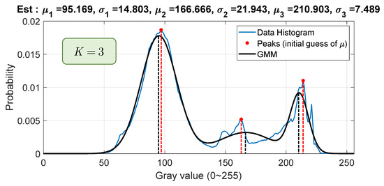
Figure 7.
Example of using peaks to determine the best initial guess of , with real-world image data.

Figure 8.
Pixel histograms and the peaks of the a* and b* channels: (a) a* channel and (b) b* channel.
Lastly, as pilots perform the landing, the complexity of the view reduces, as evidenced in Figure 9 and Figure 10. Note that the images in these figures were processed using the resizing and cropping methods introduced earlier in this section. Considering the histograms, it is shown that the number of required clusters decreases during landing. Throughout the entire landing process, if the value of K is fixed, which was determined from the first frame, some Gaussian function weights may decrease to zero, leading to a divergence in the GMM. To address this issue, a mechanism is designed to check the estimated weights () after each GMM calculation for a frame. If the system finds any weight less than 0.1, the corresponding Gaussian function with is removed, and K is adjusted to accordingly. This ensures the stability and accuracy of GMM-based image segmentation during the landing process.

Figure 9.
Image histograms of the early landing stage: (a) processed view (b) histogram of a* channel (c) histogram of b* channel.

Figure 10.
Image histograms of the late landing stage: (a) processed view, (b) histogram of a* channel and (c) histogram of b* channel.
| Algorithm 2 Initialization of GMM parameters for color images in the CIE-Lab color space. |
| Input: data in channels a* and b* |
| Output: : GMM initial guesses |
| 1: Initialize parameters for finding peaks: |
| 2: MIN_PEAK_DIST_A = |
| 3: MIN_PEAK_DIST_B = |
| 4: MIN_PEAK_HEIGHT = 0.02 |
| 5: TS = 0.0001 |
| 6: Find peaks using the 4 parameters: |
| 7: the number of peaks of |
| 8: while K is less than 3 or more than 6 do |
| 9: if K < 3 then |
| 10: TS = TS/2 |
| 11: else if K > 6 then |
| 12: TS = TS*2 |
| 13: end if |
| 14: Find peaks using the 4 parameters |
| 15: end while |
| 16: peaks of |
| 17: locations of the peaks |
| 18: = 5 |
| 19: |
To validate the developed method and evaluate the image segmentation performance, two landing simulation image sequences are used: one with a simple scene and another with a complex scene, as shown in Figure 11. The corresponding segmentation outcomes are illustrated in Figure 12 and Figure 13, while the computational time results are recorded in Table 2 and Table 3. Note that the maximum and minimum data are invalid for the phase of finding peaks since it is only performed once.

Figure 11.
Landing simulation image sequences: (a) simple scene and (b) complex scene.

Figure 12.
Segmentation results of the simple scene image sequence: (a) early stage of landing and (b) late stage of landing.

Figure 13.
Segmentation results of the complex scene image sequence: (a) early stage of landing and (b) late stage of landing.

Table 2.
The elapsed time of each phase in the simple scene.

Table 3.
The elapsed time of each phase in the complex scene.
These results demonstrate that the method successfully extracted the runway almost exclusively, and the reduction mechanism of K worked as expected. Note that in Figure 13b, the segment on the right-hand side appears fragmented. However, it actually contains the complete runway, which is obscured by a very dark shadow. Also, the segment in the complex scene contains some non-ground objects, as shown in Figure 13a, because these objects have a similar color to the runway, making it impossible to separate them through color-based clustering techniques.
Additionally, through the strategic removal of unnecessary regions and resizing the resolution, the computational demands were significantly reduced while maintaining an acceptable level of segmentation accuracy. This ensures that our proposed method can efficiently handle real-time image segmentation tasks during the landing process.
To conclude this section, an adaptive pipeline is developed to automatically determine the GMM initial guess, , and K for the first frame in the landing procedure. Then, the GMM results, including , can be fed to the GMM algorithm as the initial guesses for the next frame, as shown in Figure 14. Also, efficiency has been increased by using image pre-processing techniques, and GMM convergence for each frame has been ensured by automatically culling the redundant Gaussian functions.

Figure 14.
Finalized pipeline for optimized color image segmentation.
2.2. Integrating the Proposed Method with ORB-SLAM2
This section focuses on extracting the ground information from all the clusters generated through the GMM, which is crucial for landing attitude guidance. Additionally, the cascading effects between the input images and ORB-SLAM2 are discussed in detail.
To begin, the process of extracting the landing area is first explained. The sample inputs (Figure 15) include two test images, and the segmentation results are presented in Figure 16a,b. These results highlight the cluster containing the runway with a red rectangle. It can be observed that paved areas, like runways, have a darker appearance compared to their surroundings. Hence, the cluster with the lowest average gray value is considered a potential landing area candidate.

Figure 15.
Sample images for GMM segmentation: (a) simple scene and (b) dark scene.

Figure 16.
Segmentation results of Figure 15: (a) simple scene and (b) dark scene. Red box represents the correct desired segment.
Sometimes, insignificant fragments may also have a very low average gray value, which leads to an unsuccessful selection. As shown in Figure 16b, the average gray value of Segment 1 is 49.19, slightly lower than that of Segment 4, which is the correct desired segment. To address this, an iterative process is introduced to ensure a sufficient number of pixels in the selected cluster, avoiding selecting the wrong fragment with a low average gray value. If the criteria for the number of pixels are not met, the algorithm will select the cluster with the next lowest average gray value until it finds a suitable candidate. Finally, this extracted landing area serves as input for ORB-SLAM2.
However, feeding the image segment into ORB-SLAM2 may decrease the feature robustness and the accuracy of SLAM. First, since the feature points are restricted to a smaller region, ORB-SLAM2 lacks a sufficient number of feature points to estimate the current pose in some frames, leading to tracking loss (Figure 17a). Second, the pixels on the hard edges may be detected as FAST keypoints, as shown in Figure 17b. These keypoints have a very low reference value since they are not actual edge points in physics, which leads to a decline in feature-matching accuracy.
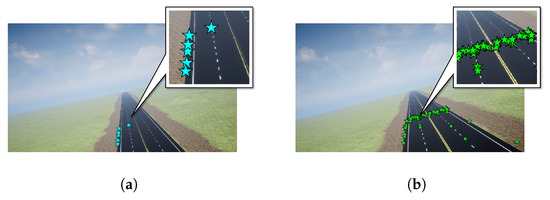
Figure 17.
Inappropriate selection of feature points: (a) feature loss and (b) features with low reference value. (The pentagrams represent the ORB feature points.)
To solve these issues, some image-processing steps are integrated after GMM segmentation. Figure 18a shows the segmented runway generated by the GMM in the form of a binary mask. The lines on the runway are culled, leaving pixel holes in this segment. As the first step, image dilation is applied using a structural element to enlarge the informative region (Figure 18b), which allows FAST to select more feature points beside the runway. Next, a Gaussian kernel is used to smooth the edges of the image segment, preventing incorrect keypoint selection on hard edges (Figure 18c), thus reducing the possibility of feature mismatches. After these additional steps, the binary mask is used to perform the pixel dot product, resulting in the filtered image (Figure 19b).

Figure 18.
The effect of image dilation and Gaussian smoothing: (a) binary mask generated from the GMM (b) after dilation (c) after Gaussian smoothing.

Figure 19.
The processed image that is fed into ORB-SLAM2: (a) original image (b) processed image.
As presented in the figure, the processed image is horizontally enlarged, including the region with strong texture, implying that FAST could select more keypoints, thus increasing the accuracy of feature matching. Also, the edges of the segment are smoothed, addressing the issue of low-reference-value feature points. The adjusted results of Figure 17 are shown in Figure 20, indicating that the two problems have been solved through these additional image-processing steps.
3. Robust Plane Fitting
As discussed previously, a safe landing relies on the proper glide slope and descending speed, which can be estimated through aircraft localization and the 3D ground map. The GMM-based method introduced in the previous chapter helps extract the ground pixels and forms the map of the landing area. Using the feature points around the current aircraft location, plane fitting methods can be introduced to calculate the plane equation and provide an appropriate glide slope. In more detail, once the aircraft succeeds in aligning its z-axis (body frame) with the normal vector of the ground, a safe glide slope can be ensured. Nonetheless, as shown in Figure 21, since the GMM-based method segments the regions according to their colors, there might still be some objects with a similar color to the ground that could not be separated, resulting in outliers during the plane fitting steps.

Figure 21.
Noisy outliers included in a 3D sparse map during a landing frame (unit: meters): (a) 3D view and (b) front view.
3.1. Outlier Removal
To address the issue of outliers, various algorithms have been developed, such as RANSAC (Random Sample Consensus) [24], MSAC (M-estimator Sample Consensus), and MLESAC (Maximum Likelihood Estimate Sample Consensus) [25]. These algorithms aim to estimate the best model from measurement data in the presence of outliers and have found widespread applications in data analysis. Compared to traditional least square methods, they do not require numerical optimization to solve nonlinear minimization problems, making them efficient, memory-saving, and suitable for real-time systems.
MSAC and MLESAC have higher accuracy compared to RANSAC [26], which can be attributed to the design of their loss functions, as shown in Equations (1)–(3):
where is the error value of each data point (indexed from 1 to n), c is the user-defined threshold for dividing inliers and outliers, is the inlier ratio, is the magnitude of inlier noise, and v is the possible range of outliers. The algorithm iterates N times, selecting the best estimated model based on the loss value. The suggested number of N is given by:
where is the probability of a failed estimation, usually set as a small number (for example, 0.001), and m is the number of data required to generate a hypothesis. Finally, is the inlier ratio, which stands for the probability of picking up an inlier from the whole dataset. In practice, the inlier ratio is usually unknown and is also a user-defined parameter. It is worth noting that the value of N relies heavily on the selection of m, and if the calculated N is too small to obtain an acceptable result in practice, N may need to be adjusted manually. These algorithms require several user-defined parameter selections, which may become the primary challenge when it comes to real-time applications.
MLESAC models inliers with a Gaussian distribution, while outliers follow a uniform distribution, resulting in high accuracy in practical problems. Therefore, in the following, MLESAC serves as the benchmark for the performance evaluation.
3.2. Iterative Weighted Plane Fitting (IWPF)
In this section, a newly designed robust plane fitting method is introduced, named iterative weighted plane fitting (IWPF). This algorithm incorporates the concept of weights to estimate the normal vector of a plane using Principal Component Analysis (PCA) and employs an iterative approach to remove outliers. IWPF aims to enhance insensitivity to user-defined parameters, improving robustness in practice.
The procedure of IWPF is listed in Algorithm 3. Using three-dimensional data as an example, it starts by initializing the weights of all data points to 1 and finding their weighted centroid. Subsequently, the weighted centroid is established as the origin, and Principal Component Analysis (PCA) is employed to identify the three principal axes of the point cloud, forming the estimated plane. Once the plane is estimated using the PCA approach, the distance of each point to the plane is computed and represented as . IWPF characterizes the noise using a zero-mean Gaussian function based on , where larger values of indicate a higher likelihood of being an outlier. This function can be expressed as:
where
By setting the threshold c, the points can be classified as either inliers or outliers, as shown in Equation (7). This physically implies that points too far from the current estimated plane are considered outliers, whereas points within the range of noise are considered inliers. Once the data points are classified, IWPF proceeds by assigning a weight of 0 to the outliers and initiates the next iteration. This entails performing PCA once again, excluding the previously identified outliers. The iteration continues until the termination condition is met, either when the maximum iteration count (N) is reached or when the change in the current estimation is less than a predefined tolerance (). Regarding the iteration tolerance, denoted as , the recommended value is 1 , and it is not the primary factor influencing the performance.
| Algorithm 3 Iterative Weighted Plane Fitting (IWPF). |
| Input: : A set of 3D point clouds, c: Threshold for inlier probability, : Tolerance |
| for iteration (suggested ), N: Maximum iteration time |
| Output: : Normal vector of the fitting plane |
| 1: Initialization. |
| 2: number of points |
| 3: weights for each point |
| 4: |
| 5: |
| 6: Indices of outliers |
| 7: Start Estimation. |
| 8: while Iteration time do |
| 9: |
| 10: Update number of inliers |
| 11: Weighted centroid |
| 12: Weighted covariance matrix |
| 13: SVD. Find the right singular matrix of A |
| which is |
| 14: Update |
| 15: Find projection points on the plane |
| 16: Define residual |
| 17: |
| 18: |
| 19: Create a Gaussian function |
| 20: For |
| consider the point as an outlier |
| 21: Update indices of outliers |
| 22: Update weights of the outliers |
| 23: if then |
| 24: break |
| 25: end if |
| 26: Update |
| 27: end while |
3.3. Comparison between IWPF and MLESAC
In this section, the Unreal Engine dataset [17] is utilized to evaluate the performance of MLESAC and IWPF. The dataset is created from two scenes with different complexities (referred to as simple and complex) and three aircraft landing paths (referred to as Ref., A, and B), resulting in a total of six scenarios. For the evaluation, two of these scenarios are used, as depicted in Figure 22, which shows that the number of feature points in the simple scene is relatively lower compared to that in the complex scene. However, the inlier ratio is notably higher. The ground in these scenes is designed to be horizontal, which means that the ground truth of the plane’s normal vector is perpendicular to the world coordinate system.
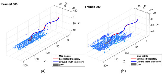
Figure 22.
Example map using Unreal Engine dataset A. (a) simple scene and (b) complex scene.
As mentioned earlier, achieving accurate landing attitude guidance involves estimating the ground slope based on the feature points situated close to and ahead of the aircraft. Hence, it becomes essential to define a bounding box that will aid in filtering the region of interest (ROI) before initiating the plane fitting process. The dimensions of the bounding box are depicted in Figure 23. As illustrated, the feature points located within the bounding box are used to perform plane fitting. Given the possibility of uneven landing terrains, it is crucial to focus exclusively on the local feature points in proximity to the aircraft rather than the global feature points. The vertical height of the bounding box is established as the maximum distance between a feature point and the camera in the vertical direction. The longitudinal length of the bounding box is set at 100 m from the camera, while the width is defined as 60 m.
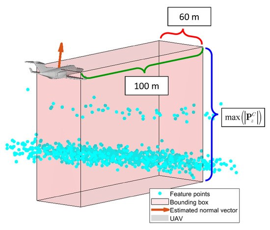
Figure 23.
Schematic of the bounding box.
First, the error of the estimated normal vector for MLESAC is shown in Table 4. Overall, the performance varies significantly under different values, showing that MLESAC is sensitive to user-defined parameters. On the other hand, inappropriate selection of the inlier noise level () could be fatal to the system. However, during an emergency landing, it is impossible to obtain information about noise in advance, which implies that it is not suitable to use MLESAC in the landing assistance system. Second, the error of the estimated normal vector for the proposed algorithm, IWPF, under different user-defined parameters c is listed in Table 5. The average error is within 1.21 degrees, and the performance is stable and not affected by the selection of c.

Table 4.
Error (degrees) for MLESAC in the simple scene (S) and the complex scene (C).

Table 5.
Error (degrees) for IWPF in the simple scene (S) and the complex scene (C).
In conclusion, the robustness of IWPF has been substantiated through these tests, with its performance remaining resilient to the choice of the threshold parameter, c. Figure 24 summarizes the methodologies from Section 2 and Section 3, comprising three main blocks. Firstly, the GMM ground extraction block aims to extract the ground image from the stereo camera input. Second, ORB-SLAM2 produces the aircraft’s pose and a 3D ground map, which can be used by the third block to calculate a suitable relative glide slope through the robust IWPF algorithm, aiding the pilot in a safe landing.
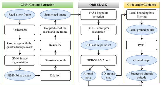
Figure 24.
Full flowchart of the system.
4. Results and Discussion
In this section, the developed algorithms are validated on all six Unreal Engine datasets: Ref., A, B, Ref_city, A_city, and B_city.
First, for the 6DoF localization, the RMSE is shown in Table 6. As previously discussed, since the number of feature points is fewer in the simple scene, the overall performance of ORB-SLAM2 declined slightly compared to the complex scene. Second, for the ground slope estimation, the error values of IWPF are shown in Table 7 and Figure 25, showing that the proposed algorithms successfully provided the glide angle. In addition, the maximum error only occurred in the first few frames after the system initialized, where the inlier ratio of feature points was significantly lower, leading to the failed estimations of IWPF. Considering the presented simulation results, it can be concluded that the system should accumulate at least 500 feature points to ensure an accurate glide slope estimation. With this additional step, the results show an average error of approximately 1 degree. Note that for Path B, which simulates heavy landings (datasets B and B_city), the results during the last part are invalid since the camera was too close to the ground and could not capture any image features.

Table 6.
RMSE of 6DoF localization. Translations x, y, and z are in meters, while rotations , , and are in degrees.

Table 7.
Error (degrees) of IWPF. Avg.* = the average after accumulating 500 feature points.

Figure 25.
The number of feature points used for plane fitting and the corresponding error: (a) UE_Ref, (b) UE_Ref_city, (c) UE_A, (d) UE_A_city, (e) UE_B and (f) UE_B_city (UE_B and UE_B_city encountered tracking loss in the last part as the camera was too close to the ground).
Next, we further used a reference path designed in [17] as a benchmark to judge whether the aircraft’s height was safe and aligned with the center of the runway, such that the pilot would receive an alarm when the aircraft’s status was at risk. As illustrated in Figure 2b, once the aircraft started to descend, a virtual landing tunnel popped up, representing the aforementioned reference path. Additionally, we used Paths A and B to demonstrate the capability of the proposed alarm system, as shown in Figure 26 and Figure 27, respectively. The simulation results show that the system successfully indicated the aircraft’s position status using real-time localization data. Also, it should be noted that in Figure 27, the alarm flag in the last part was invalid due to vision failure, as mentioned previously.

Figure 26.
Center–alignment alarm test: (a) UE_A (b) UE_A_city.
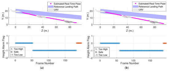
Figure 27.
Height alarm test: (a) UE_B (b) UE_B_city (encountered tracking loss in the last part as the camera was too close to the ground).
Combining this alarm system with the landing attitude guidance feature introduced previously, the system was able to provide the pilot with an intuitive decision-making interface, ensuring safety on unknown uneven runways. For real-time systems, a high update rate is also required. These simulations were performed using MATLAB, as mentioned in [17], and the system’s operation time per frame is summarized in Table 8.

Table 8.
System’s operation time per frame.
5. Conclusions and Future Work
In this paper, the critical need for an onboard standalone decision-aid landing assist system is addressed, particularly for fixed-wing aircraft emergency landings in the absence of additional external navigation systems. Drawing inspiration from naked-eye landings, a stereo vision-assisted landing system is developed, which is capable of guiding pilots to safely land on diverse runways and highways. This system adapts the ORB-SLAM2 technique as the fundamental framework for environmental perception and overcomes the challenge of extracting the desired ground points, which traditional SLAM frameworks struggle with. This work also designs a GMM-based color image segmentation method for land extraction, and the segmented land image is used as input for ORB-SLAM2. The proposed method effectively extracts the ground region, and the corresponding normal vector can be calculated precisely using the proposed IWPF. With the robust normal vector estimation, pilots can evaluate whether the aircraft’s landing direction is aligned with the surface and, therefore, unexpected landing accidents can be avoided. Finally, different flight scenarios are considered to evaluate the effectiveness and feasibility of the proposed decision-aid landing system.
For future work, considering the implementation in the real world, one potential method to enhance the system’s performance is to utilize an Inertial Measurement Unit (IMU) capable of providing a high update rate for Euler angle estimation. The fusion of sensor data using an Extended Kalman Filter (EKF) becomes a significant consideration for achieving optimal results.
Author Contributions
Conceptualization, C.-C.P.; Methodology, C.-C.P.; Software, C.-S.C. and C.-C.P.; Validation, C.-S.C.; Formal analysis, C.-S.C. and C.-C.P.; Investigation, C.-S.C. and C.-C.P.; Writing—original draft, C.-S.C.; Writing—review & editing, C.-C.P.; Visualization, C.-S.C.; Supervision, C.-C.P.; Project administration, C.-C.P.; Funding acquisition, C.-C.P. All authors have read and agreed to the published version of the manuscript.
Funding
National Science and Technology Council Grant Numbers: NSTC 111-2923-E-006-004-MY3 and NSTC 112-2221-E-006-104-MY3.
Data Availability Statement
The data that support the findings of this study are available from the corresponding author upon reasonable request.
Conflicts of Interest
The authors declare no conflicts of interest.
References
- Airbus. Accidents by Flight Phase. Available online: https://accidentstats.airbus.com/accidents-by-flight-phase/ (accessed on 2 May 2024).
- News, C. Small Plane Makes Hard Landing on Highway 91 in Delta. Available online: https://www.cbc.ca/news/canada/british-columbia/small-plane-makes-hard-landing-on-highway-91-in-delta-1.3045037 (accessed on 2 May 2024).
- Staff, K. UPDATE: Plane Forced to Land Due Mechanical Failure Hits Power Line, Fire Officials Say. Available online: https://www.ksby.com/news/local-news/plane-forced-to-land-due-mechanical-failure-hits-power-line-fire-officials-say (accessed on 2 May 2024).
- News, G. Plane’s Emergency Landing Captured on Police Dashboard Camera. Available online: https://www.youtube.com/watch?v=xIhj_xFKtM4 (accessed on 2 May 2024).
- News, G. Video Shows Pilot Landing Stricken Small Plane on Highway. Available online: https://www.youtube.com/watch?v=uwkgj6PqUgI (accessed on 2 May 2024).
- National Transportation Safety Board. Crash during Nonprecision Instrument Approach to Landing, Execuflight Flight 1526, British Aerospace HS 125-700A, N237WR, Akron, Ohio, 10 November 2015; National Transportation Safety Board: Washington, DC, USA, 2016. Available online: https://www.ntsb.gov/investigations/AccidentReports/Reports/AAR1603.pdf (accessed on 3 May 2024).
- Wikipedia. Instrument Landing System. 2022. Available online: https://en.wikipedia.org/wiki/Instrument_landing_system (accessed on 3 May 2024).
- Mbaocha, C.; Ekwueme, E.; Nosiri, O.; Chukwuchekwa, N. Aircraft Visibility Improvement with Dedicated Instrument Landing System (ILS). 2018. Available online: https://www.researchgate.net/publication/327964605 (accessed on 3 May 2024).
- Lu, Y.; Xue, Z.; Xia, G.S.; Zhang, L. A survey on vision-based UAV navigation. Geo-Spat. Inf. Sci. 2018, 21, 21–32. [Google Scholar] [CrossRef]
- Chen, C.L.; He, R.; Peng, C.C. Development of an Online Adaptive Parameter Tuning vSLAM Algorithm for UAVs in GPS-Denied Environments. Sensors 2022, 22, 8067. [Google Scholar] [CrossRef] [PubMed]
- Schlegel, D.; Colosi, M.; Grisetti, G. ProSLAM: Graph SLAM from a Programmer’s Perspective. In Proceedings of the 2018 IEEE International Conference on Robotics and Automation (ICRA), Brisbane, Australia, 21–25 May 2018; pp. 3833–3840. [Google Scholar] [CrossRef]
- Gao, B.; Lang, H.; Ren, J. Stereo Visual SLAM for Autonomous Vehicles: A Review. In Proceedings of the 2020 IEEE International Conference on Systems, Man, and Cybernetics (SMC), Toronto, ON, Canada, 11–14 October 2020; pp. 1316–1322. [Google Scholar] [CrossRef]
- Calonder, M.; Lepetit, V.; Strecha, C.; Fua, P. BRIEF: Binary Robust Independent Elementary Features. In Computer Vision–ECCV 2010: 11th European Conference on Computer Vision, Heraklion, Crete, Greece, 5–11 September 2010; Springer: Berlin/Heidelberg, Germany, 2010; Volume 6314, pp. 778–792. [Google Scholar] [CrossRef]
- Mur-Artal, R.; Montiel, J.M.M.; Tardós, J.D. ORB-SLAM: A Versatile and Accurate Monocular SLAM System. IEEE Trans. Robot. 2015, 31, 1147–1163. [Google Scholar] [CrossRef]
- Muja, M.; Lowe, D. Fast Approximate Nearest Neighbors with Automatic Algorithm Configuration. In Proceedings of the Fourth International Conference on Computer Vision Theory and Applications, Lisbon, Portugal, 5–8 February 2009; pp. 331–340. [Google Scholar]
- Mur-Artal, R.; Tardós, J.D. ORB-SLAM2: An Open-Source SLAM System for Monocular, Stereo, and RGB-D Cameras. IEEE Trans. Robot. 2017, 33, 1255–1262. [Google Scholar] [CrossRef]
- Peng, C.C.; He, R.; Chuang, C.S. Evaluation of ORB-SLAM based Stereo Vision for the Aircraft Landing Status Detection. In Proceedings of the IECON 2022—48th Annual Conference of the IEEE Industrial Electronics Society, Brussels, Belgium, 17–20 October 2022; pp. 1–6. [Google Scholar] [CrossRef]
- Jang, C.; Lee, S.; Choi, C.; Kim, Y.K. Realtime robust curved lane detection algorithm using Gaussian mixture model. J. Inst. Control Robot. Syst. 2016, 22, 1–7. [Google Scholar] [CrossRef]
- Bi, H.; Tang, H.; Yang, G.; Shu, H.; Dillenseger, J.L. Accurate image segmentation using Gaussian mixture model with saliency map. Pattern Anal. Appl. 2018, 21, 869–878. [Google Scholar] [CrossRef]
- Yang, X.; Chen, L.; Cao, D. Design of Integrated Road Perception and Lane Detection System for Driver Intention Inference. In Advanced Driver Intention Inference; Elsevier: Amsterdam, The Netherlands, 2020; pp. 77–98. [Google Scholar]
- Yang, W.; Li, H.; Liu, J.; Xie, S.; Luo, J. A sea-sky-line detection method based on Gaussian mixture models and image texture features. Int. J. Adv. Robot. Syst. 2019, 16, 1729881419892116. [Google Scholar] [CrossRef]
- Bakti, R.Y.; Areni, I.S.; Prayogi, A.A. Vehicle detection and tracking using gaussian mixture model and kalman filter. In Proceedings of the 2016 International Conference on Computational Intelligence and Cybernetics, Makassar, Indonesia, 22–24 November 2016; pp. 115–119. [Google Scholar]
- MathWorks. Findpeaks. 2022. Available online: https://www.mathworks.com/help/signal/ug/find-peaks-in-data.html (accessed on 3 May 2024).
- Fischler, M.A.; Bolles, R.C. Random sample consensus: A paradigm for model fitting with applications to image analysis and automated cartography. Commun. ACM 1981, 24, 381–395. [Google Scholar] [CrossRef]
- Torr, P.H.; Zisserman, A. MLESAC: A new robust estimator with application to estimating image geometry. Comput. Vis. Image Underst. 2000, 78, 138–156. [Google Scholar] [CrossRef]
- Choi, S.; Kim, T.; Yu, W. Performance evaluation of RANSAC family. In Proceedings of the British Machine Vision Conference, London, UK, 7–10 September 2009; pp. 1–12. [Google Scholar]
Disclaimer/Publisher’s Note: The statements, opinions and data contained in all publications are solely those of the individual author(s) and contributor(s) and not of MDPI and/or the editor(s). MDPI and/or the editor(s) disclaim responsibility for any injury to people or property resulting from any ideas, methods, instructions or products referred to in the content. |
© 2024 by the authors. Licensee MDPI, Basel, Switzerland. This article is an open access article distributed under the terms and conditions of the Creative Commons Attribution (CC BY) license (https://creativecommons.org/licenses/by/4.0/).
