LoRa Radio Frequency Fingerprinting with Residual of Variational Mode Decomposition and Hybrid Machine-Learning/Deep-Learning Optimization

Abstract

Radio Frequency Fingerprinting (RFF) refers to the technique for identifying and classifying wireless devices on the basis of their physical characteristics, which appear in the digital signal transmitted in space. Small differences in the radio frequency front-end of the wireless devices are generated across the same wireless device model during the implementation and manufacturing process. These differences create small variations in the transmitted signal, even if the wireless device is still compliant with the wireless standard. By using data analysis and machine-learning algorithms, it is possible to classify different electronic devices on the basis of these variations. This technique has been well proven in the literature, but research is continuing to improve the classification performance, robustness to noise, and computing efficiency. Recently, Deep Learning (DL) has been applied to RFF with considerable success. In particular, the combination of time-frequency representations and Convolutional Neural Networks (CNN) has been particularly effective, but this comes at a great computational cost because of the size of the time-frequency representation and the computing time of CNN. This problem is particularly challenging for wireless standards, where the data to be analyzed is extensive (e.g., long preambles) as in the case of the LoRa (Long Range) wireless standard. This paper proposes a novel approach where two pre-processing steps are adopted to (1) improve the classification performance and (2) to decrease the computing time. The steps are based on the application of Variational Mode Decomposition (VMD) where (in opposition to the known literature) the residual of the VMD application is used instead of the extracted modes. The concept is to remove the modes, which are common among the LoRa devices, and keep with the residuals the unique intrinsic features, which are related to the fingerprints. Then, the spectrogram is applied to the residual component. Even after this step, the computing complexity of applying CNN to the spectrogram is high. This paper proposes a novel step where only segments of the spectrogram are used as input to CNN. The segments are selected using a machine-learning approach applied to the features extracted from the spectrogram using the Local Binary Pattern (LBP). The approach is applied to a recent LoRa radio frequency fingerprinting public data set, where it is shown to significantly outperform the baseline approach based on the full use of the spectrogram of the original signal in terms of both classification performance and computing complexity.

1. Introduction

Radio frequency fingerprinting is a technique for the identification and authentication of wireless devices, which has received increased attention from the research community in recent years. As described in [1], the security of wireless networks is a very important aspect to ensure the trust of wireless services, which are now pervasive in our society. In this context, networking and security protocols assume that the identities of users and devices are distinct and unique, but this can be violated by cybersecurity attackers, who can spoof the identity of a wireless device. To address such attacks, cryptographic-based approaches are proposed in the research literature and communication infrastructures. Such approaches usually have the goal of binding a device or a node in a wireless communication system with a cryptographic identity of a certificate. On the other side, the deployment of cryptographic frameworks can be costly because of the need to implement processes like key distribution and key management, which can be particularly cumbersome in Internet of Things (IoT) systems like the LoRa devices considered in this study because of the computing limitations of such devices [2]. Recently, RFF has been proposed by various researchers as an alternative or complementary means of cryptographic identification for wireless communications [1,3,4].

This technique is based on the exploitation of the intrinsic physical differences among wireless devices supporting the same wireless standard. These physical differences are created during the manufacturing process or the design process due to the use of different materials or different configurations of electronic components, especially in the radio frequency front-end. Even if such differences do not usually hamper compliance to the wireless standard, they alter the signal in space generated by the wireless device in such a way that the device itself can be identified by the analysis of the signal. The advantage of RFF in comparison to cryptographic techniques is that it does not require the distribution and secure storing of cryptographic materials (which is particularly beneficial for IoT environments) and that it is based on the unique physical properties of the wireless device [3]. On the other side, the identification is based on probability derived from the matching of the fingerprints, and research is still progressing in improving such probability in terms of accuracy and required computing time [1,4], which is also the objective of this study.

The analysis of the signal and the identification of the wireless devices can be implemented as a pattern recognition problem, and various techniques can be used, including the application of Machine Lerning (ML), DL algorithms to a feature space created from the application of hand-crafted features (e.g., entropy, variance) to the time or spectral domain representation of the signal. Some studies have implemented a pre-processing step on the signals generated by the emitters to enhance the performance of ML. For example, the authors in [5] applied VMD to decompose the signal in modes to generate a more comprehensive feature space. The approaches based on ML are usually computing efficient, but they rely on the identification of hand-crafted features, which may not be optimal for the specific data set. DL has demonstrated a superior classification performance to the so called ‘shallow’ ML algorithms in various RFF studies, as described in a recent survey [3]. The advantage of DL is also that features are extracted automatically. On the other side, DL requires significant computing resources, particularly for the training time. Some DL algorithms and architectures like CNN are particularly powerful for the classification of images, and some recent studies have converted the 1D initial signal from the emitter to a 2D image using various techniques, like the application of the spectrogram [6], but they may significantly increase the size of the input data to the DL algorithm, thus increasing the computing time even more.

This paper proposes a hybrid (combination of ML and DL) approach where various elements are brought together to enhance the performance of RFF:

• The VMD is applied as a pre-processing step to highlight the fingerprints from the signal. The residual of the application of VMD to the signals of the emitters to be classified is used for RFF rather than the generated modes, as is commonly done in the literature. This pre-processing step is proposed to remove the signal modes, which are common to all the emitters and highlight the fingerprints for further processing.
• The spectrogram is used to obtain a 2D representation of the signal.
• On the spectrograms, a novel image reduction step is applied, which is based on the application of Shannon entropy and LBP image processing features to select the most discriminating Region Of Interest (ROI) so that they can be assembled to generate a new 2D input to a multi-headed CNN. This step improves classification performance and decreases its computing time.
• A multi-headed CNN is used to perform the classification and implement the final step of RFF.

To the knowledge of the authors, this combination of elements is novel for the problem of RFF. The proposed approach is applied to a recent public data set of LoRa devices [6].

This paper has the following structure: Section 2 summarizes the research literature on RFF, with a particular focus on the use of mode decomposition methods for RFF. Section 3 describes the material and methods used to implement the proposed approach. In particular, this section describes the elements in the methodology: the structural diagram of the procedures, the used public data set, the definition of the LBP and VMD, the computing platform used to perform the experiments, CNN architectures, and the evaluation metrics. Section 4 provides the results of the proposed approach on the described data set and conducts an analysis of the findings. Finally, Section 5 provides the conclusions and outlines future developments.

2. Related Work

The literature on radio frequency fingerprinting is quite vast, and many studies have been published in recent years, as described in recent surveys like [3,7]. While initial studies [8] used handcrafted features in combination with ML to implement the classification, the application of DL to RFF was demonstrated to be highly successful in [9,10,11]. For this reason, this study also uses DL but in combination with the application of VMD.

The rest of this section focuses on the application of VMD to RFF. The predominant use of VMD in this context is to decompose the original signal in modes on which handcrafted features are applied to generate a feature space. ML algorithms are then used to perform the classification and identification of wireless devices. Two different data sets of DSRC (ITS G5 standard [12] used for vehicular applications) devices and IoT devices were used in the study. This is the approach used in [13], where VMD was used in combination with features like variance, entropy, skewness, and kurtosis to create a feature space where Support Vector Machine (SVM) and K-Nearest Neighbor (KNN) were applied. The results from [13] show that this approach was able to outperform both the use of the original signal representation in the time domain and frequency domain or the use of Empirical Mode Decomposition (EMD), which is another mode decomposition algorithm, which predates VMD and which was used in [14].

Similarly, the authors in [5] used VMD in combination with spectral features and KNN on a data set of emitter devices to implement RFF. The study presented in [5] considered both single-hop emitter devices and multi-hop relaying devices with a comparable performance.

Another study exploiting VMD for RFF was [15], where devices implementing the Bluetooth wireless standard [16] were used. As in the previously cited paper, Higher Order Statistics (HOS), namely variance, skewness, and kurtosis, are calculated from the instantaneous amplitude, frequency, and phase of the modes generated by the application of VMD. The Linear Support Vector Machine (LSVM) was used to perform classification.

A similar work is [17], where handcrafted features were applied to the transient portion of the signal generated by Bluetooth devices to generate a feature space, where the LSVM was used to implement RFF.

Another approach based on VMD, but using a different set of features, was proposed in [18], where the Hilbert transform was applied to the modes originating from the VMD decomposition of signals generated by ZigBee devices. The Hilbert transform is used to generate images from the modes on which Histogram of Oriented Gradient (HOG) features are applied to generate a feature space. Then, KNN is applied to implement RFF and classify the ZigBee devices. As described in the subsequent sections, this study also applied images-related features, but it uses LBP instead of HOG to generate a more compact feature space. In addition, the LBP features are applied to a spectrogram instead of the result of the Hilbert transform, and they are not used for the main classification task as in [18], but to reduce the size of the images given as input to the DL algorithm. The VMD is also used to generate the residual rather than the modes themselves, and DL was not used in [18].

Another set of features (still in combination with VMD) was used in [19], where the Teager operator was applied and the energy and box dimension were extracted as fingerprint features to be given in input to SVM for the classification of the emitters.

Reviewing the studies presented above, we can conclude that no study has applied the analysis to the residual of the VMD rather than the modes generated by the VMD. In addition, all the papers presented so far did not apply DL in combination with VMD.

The application of DL to RFF is quite recent, but it has shown a higher accuracy in comparison to ML algorithms like SVM or KNN used in the references cited above at the cost of an increased computing complexity and time. In particular, a popular approach in the research literature is to combine time-frequency distributions with DL algorithms, which are particularly effective in the analysis of images like CNN. This approach was used with various time-frequency transforms. In [6], which proposed the same data set used in this study, a spectrogram was used in combination with CNN, but the VMD was not used to pre-process the signals. This step provides a significant advantage, as shown in Section 4 of this paper. A similar approach with the spectrogram was also used in [20], still on LoRa devices without using the VMD as well. The relevance of the application of RFF to LoRa devices is also shown in [21], where CNN was used together with a spectral domain (based on the application of the Fast Fourier Transform (FFT) in the study) representation of the signal as it was shown to outperform the original time domain representation.

One key issue of the application of time-frequency transform together with DL is that the size of the input data can be significantly large (in comparison with the original time representation). It would then be beneficial to reduce the input of images created with the application of the time-frequency transform to a smaller size while preserving the discriminating power. One possibility would be to use computing-efficient features and ‘shallow’ ML algorithms to identify ROIs, which are more discriminating than others, and then give only the assembled ROIs to the DL algorithm. This approach was applied recently in [22] but only to 1D spectral domain representations (i.e., application of the FFT) and not to time-frequency transforms. In other fields, the use of a hybrid approach, which combines handcrafted features and DL to improve computing efficiency and classification performance, has recently been proposed for generic image processing in [23], though with different features than in this study.

In relation to the cited literature, this paper proposes a novel approach, based on the application of image processing features, to reduce the spectral domain representation given in input to the DL algorithm to enhance classification accuracy and reduce computing time.

3. Materials and Methods

3.1. Methodology

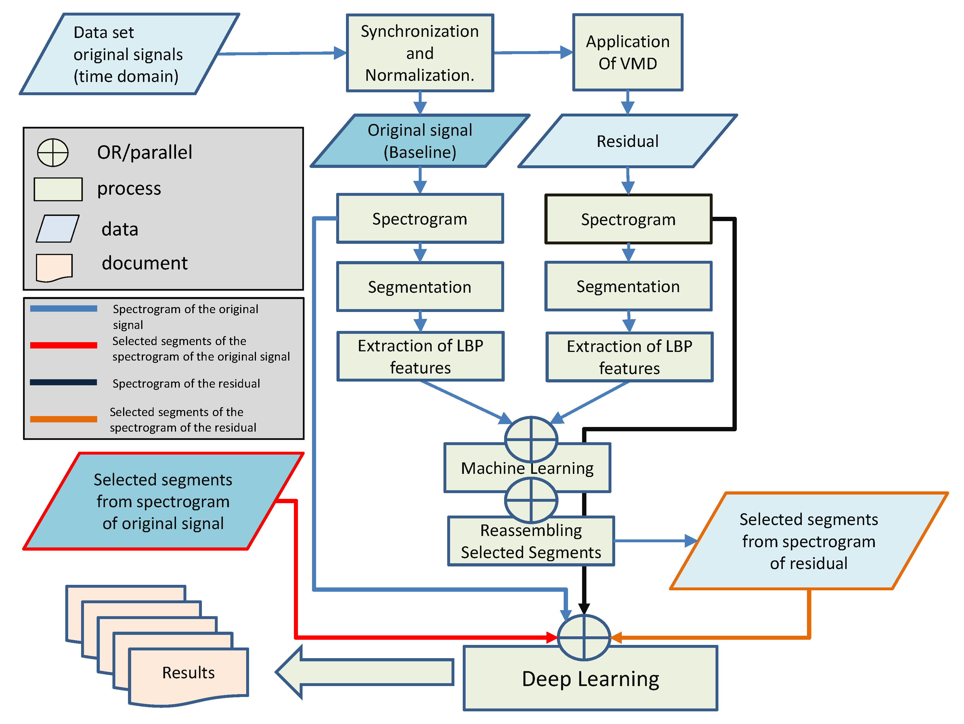
The overall methodology of the proposed approach is shown in Figure 1, where the structural diagram of procedures is pictorially represented. The different color codes are used to show the different paths to generate the results, which are compared and analyzed in Section 4. The paths are, respectively: (1) spectrogram with the original signal (blue), (2) spectrogram with the residual from the VMD (black), (3) reduced spectrogram (selected segments) with the original signal (red), and (4) reduced spectrogram (selected segments) with the residual from the VMD (magenta). The spectrogram is reduced thanks to the technique described in the following steps.

In the first step, the signals of the LoRa devices are synchronized and normalized. A set of $N_D=10$ LoRa devices are used in this study, as described in Section 3.2. For each LoRa device, $N_B=500$ bursts were generated for a total of 5000 bursts. Then, the VMD was applied to each burst with a value of $\alpha =2000$ and the number of modes, $N_M$, which is a hyper-parameter in this study. The residual was extracted from the signals after the main modes were identified. For this purpose, the MATLAB 2022b vmd function was used from the Signal Processing toolbox, which is in turn based on the theoretical framework defined in [24].

The value of $\alpha$ was identified on the basis of the LoRa modulation and the settings of the data set. Because the study is focused on the residual, the number of modes is kept low within the following range: $N_M=[2,\cdots ,5]$. A large number of modes may include the fingerprints, which are needed to classify the LoRa devices, while a relatively small number of modes would include the common elements of the signals, which we want to remove. Another hyper-parameter in the study is the window size, $W_S$, used to generate the spectrogram. This value was chosen following the settings defined in [6], where the data set was initially proposed. In [6], a Gaussian window of $W_S=256$ was used, with an overlapping of 128. In this study, we also added the Gaussian window of $W_S=128$ with an overlapping of 64.

A representation of the signal is shown in Figure 2, together with one-sided spectrograms with $W_S=256$. The spectrograms are generated by using the MATLAB 2022b stft function. These images are provided only as a reference. As explained in the subsequent sections of this paper, a two-sided centered spectrogram is used as input to the DL algorithm to enhance and center the relevant content of the spectrogram.

Then, the other element of the proposed approach is applied. Each spectrogram is converted to a grayscale image and sub-divided into 32 rectangles. The initial image is divided by 4 for the frequency dimension and 8 for the time dimension. In each square, the LBP values were calculated in addition to the Shannon entropy of the rectangular image. This creates a feature space of size $N_D*N_B*60$ (59 features of the LBP plus the Shannon entropy) for each rectangle. For each of the 32 rectangles, the accuracy was calculated using a Decision Tree (DT) algorithm, with the maximum number of splits equal to 12 (this was found to be the optimal value in a range from 1 to 20).

The 8 best results are adopted to represent the optimal set of rectangles, which are reassembled to create a new image, whose size is one-quarter of the original one. This novel step not only decreases the overall classification time, because the DL algorithm has to process smaller images, but it may also enhance the classification performance. This assumption will be proven by the findings shown in the Section 4. Note that the value of 8 was chosen as a compromise between the need to obtain a significant reduction in the input data while still preserving significant data for the classification. This could also be a hyper-parameter to tune, but we preferred to focus the analysis on other hyper-parameters, namely the number of modes, $N_M$, in the VMD and the window size, $W_S$, of the spectrogram.

3.2. Data Set

This section describes the data set used in this study. The data set was generated by the authors of [6] and it is based on the identification of wireless devices supporting the LoRa wireless communication standard [25].

LoRa uses Frequency Shift Chirp Modulation (FSCM), which uses chirps for communication [26]. In the context of wireless communications, a chirp can be defined as a signal in which the communication frequency increases (up-chirp) or decreases (down-chirp) with time. The instantaneous frequency of the LoRa signal changes continuously over time, and a basic LoRa symbol (up-chirp) can be written as:

$$u\left(t\right)=A^{j\times 2\pi \left(-\frac{B}{2}+\frac{B}{2T}t\right)t},$$

(1)

where A and B represent, respectively, the amplitude and signal bandwidth of the LoRa signal. T is the duration of the LoRa symbol, which can be represented as:

$$T=2^{SF}/B,$$

(2)

where SF is the spreading factor. There are eight repeating up-chirps at the beginning of a LoRa packet called the preamble, which is identical in every LoRa packet regardless of the device type. Then, the preamble can be used for RFF because it is invariant to the data transmitted by the LoRa devices, which may bias the extraction of the RFF.

The signals collected by the authors of [6] need to be pre-processed so that they can be exploited for the RFF implementation. In particular, they need to be synchronized, compensated for Carrier Frequency Offset (CFO), and normalized. The reasons for these pre-processing steps are to avoid the introduction of bias in the implementation of RFF because the DL algorithm used for classification may be confused by the different power levels of the signal (which requires normalization) and misrepresent the wireless devices. In a similar way, the lack of synchronization or CFO may cause similar effects.

The phase information of the LoRa signal in the data set is noisy and can be affected by several issues, such as phase noise, CFO, and sampling time offset. Therefore, only the spectrogram is used in this study, which is consistent with the methodology proposed in [6]. This study uses the fingerprints from 10 LoRa devices from the data set provided by the authors in [6] from the training data set. In the data set, 500 bursts of each LoRa device are provided. Then, a total of $10\times 500$ burst (5000 bursts) are used in the study. Each burst has a size of 8192 samples. This number of devices is consistent with other similar studies using LoRa devices for RF fingerprints, like [27], where 10 devices were also used, or other RFF studies like [13],where 11 devices were used, and [9], where 5 devices were used.

3.3. Local Binary Pattern

This section provides the definition of LBP as it was used in this paper to implement the dimensionality reduction. The LBP is a nonparametric operator for the description of local image features. It has the benefit of being rotation invariant and translation invariant [28]. The LBP of a cell is calculated in the following way. For a center pixel in an image or a cell (in this study, the section of the image identified in Section 3 and the cell size and image size are the same), and the pixel is compared to each of its 8 neighbors. Where the value of the center pixel is greater than the neighbor’s value, a value of 0 is recorded. Otherwise, a value of 1 is recorded. This gives an 8-digit binary number as in the following Equation (3), where $x_c$ and $y_c$ are the coordinates of the center pixel and $i_n$ is the gray value of the pixels of its eight neighbors; N is the number of neighbors and the neighbor is identified with the parameter n.

$$LBP(x_c,y_c)=\sum _{n=0}^{7}Ne(i_n-i_c)*2^n.$$

(3)

In the next step of the LBP algorithm, the histogram is computed, over the cell, of the frequency of each “number” occurring. Then, the normalized histograms of all cells are concatenated to give the feature vector for the entire window.

The rationale for using the LBP in this context is that the differences in the spectrogram may indicate the slight variations in time or frequency between the signals generated by the wireless devices that are related to fingerprints. The additional advantage of LBP in the comparison of other image processing features (e.g., Scale-Invariant Feature Transform (SIFT) or HOG) is that the computing complexity is relatively limited. For the sections of the spectrogram images considered in this study, the generated feature space is also limited (i.e., 59 features).

The MATLAB 2022b implementation of LBP provided by the authors of [29] was used in this study.

3.4. Deep-Learning Architecture

This section describes the DL architecture used in this study.

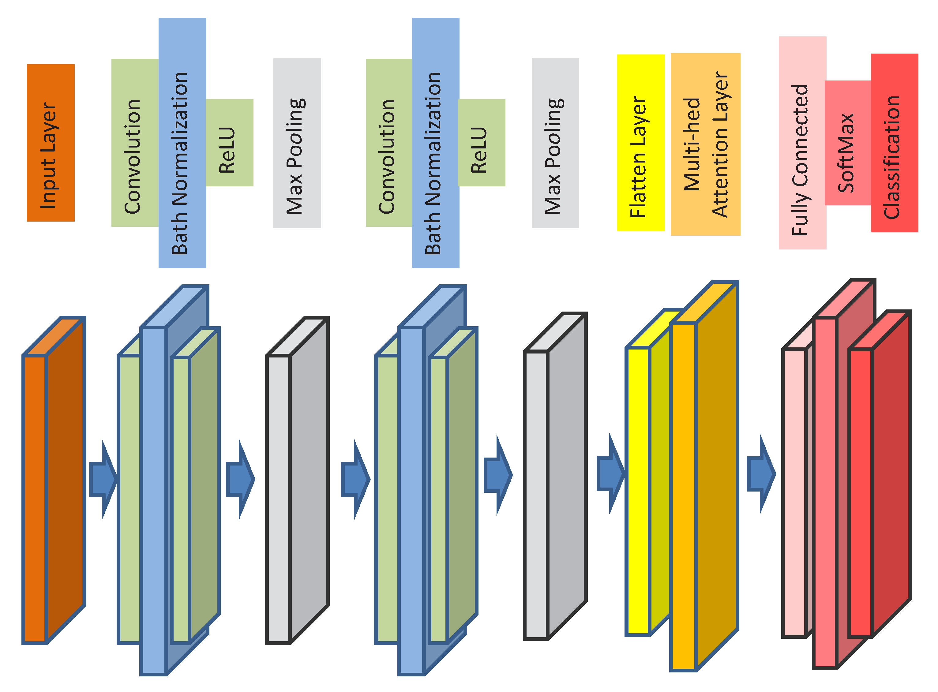
A CNN architecture with two convolutional layers and multi-head attention was used to implement the classification, as shown in Figure 3.

The values of the parameters of the DL architecture used in this study are shown in

Table 1. List of the CNN parameters used in this study.

CNN Parameter	Value
CNN solver algorithm	Adam
Number of Convolutional Layers	2
Width and filter size of the 1st convolutional layer	32,32
Number of filters in the 1st convolutional layer	32,32
With and filter size of the 2nd convolutional layer	12,12
Number of filters in the 2nd convolutional layer	32,32
1st pooling layer	Max pooling (4,4) with Stride (2,2)
2nd pooling layer	Max pooling (4,4) with Stride (2,2)
Activation function	ReLu
Number of heads in the attention layer	8
Number of channels for keys and queries in the attention layer	64
Maximum number of epochs	180

. Some values of the CNN parameters were guided by the size of the spectrogram image itself, like the width and the filter size (i.e., 32, as shown in the subsequent table), while other parameters were tuned according to a range of values to achieve the optimal performance for the majority of cases. In particular, the Adaptive moment estimation (Adam) solver was chosen over the Stochastic Gradient Descent with Momentum (SGDM) and the Root mean square propagation (RMSProp). The maximum pooling operation was preferred to the average pooling operation, and the optimal number of heads was chosen in a range of 4 to 10 in steps of 2. Rectified Linear Unit (ReLu) was used as an activation function. Other DL architectures could also be used, including the pre-trained CNN models, but we would like to highlight that the purpose of this study was not to compare DL architectures (which also include specific constraints on the size of the input images and it may not be suitable for this specific context), but to evaluate the performance improvement of the use of the residuals from VMD and the image reduction step with the LBP features and the Shannon entropy feature.

The evaluation metrics used in this study are accuracy, F-score, and the overall computation time. In this study, the computational time of the proposed approach is the sum of the computational times of the different methodological steps described in Section 3.1.

The accuracy is defined by the following equation:

$$Accuracy=\frac{TP+TN}{TP+TN+FP+FN}.$$

(4)

The F-score is the harmonic mean of precision and recall and it is defined by the following equation:

$$F-score=\frac{2*TP}{2*TP+FP+FN},$$

(5)

where TP is the number of True Positives, TN is the number of True Negatives, FP is the number of False Positives, and FN is the number of False Negatives.

The computational time is calculated in a normalized way using as a unitary value the smallest computing time among the various steps described in Section 3.1.

3.5. Variational Mode Decomposition

The VMD technique belongs to the family of mode decomposition algorithms and it was initially proposed in [24]. In comparison to other mode decomposition algorithms like EMD, VMD has a number of significant advantages, including the aspect that it is non-recursive, adaptive, and based on a quasi-orthogonal signal decomposition.

The main goal of the VMD algorithm is to decompose a multi-component signal in a discrete number of sub-signals, which are called modes or Intrinsic Mode Functions (IMF) with limited bandwidth in the spectral domain, assuming each mode to be mostly compact around a center pulsation, ${\omega }_k$. In the rest of this paper, we use the term mode to indicate the IMF.

The bandwidth of a mode, $u_k$, is assessed in the following way [24]: (a) using the Hilbert transform, calculate for each mode the associated analytical signal and obtain a unilateral frequency spectrum; (b) for each mode, shift the mode’s frequency spectrum to baseband by mixing with an exponential, tuned to the respective estimated center frequency; and (c) estimate the bandwidth through the $H^1$ Gaussian smoothness of the demodulated signal (the squared $L^2$-norm of the gradient). Therefore, for a given signal, $s\left(t\right)$, with k modes, $u_k$, and related center frequencies, ${\omega }_k$, the variational problem is expressed as follows:

$$\underset{\left\{u_k\right\},\left\{{\omega }_k\right\}}{min}\left\{\sum _k{∥{\partial }_t\left[\left(\delta \left(t\right)+\frac{j}{\pi t}\right)*u_k\left(t\right)\right]e^{-j{\omega }_{k}t}∥}_2^2\right\},$$

(6)

where $\delta$ is the Dirac distribution, * denotes convolution, and s is subject to ${\sum }_k{u}_k=s$.

The VMD has two main hyper-parameters to tune. The first hyper-parameter is the $\alpha$ parameter from Equation (15) in [24], which is the balancing parameter of the data-fidelity constraint, and the second hyper-parameter is the number of modes, k.

The hyper-parameter $\alpha$ is usually related to the frequency structure of the signal itself, which is known in this case on the basis of the LoRa standard. [25] A value of $\alpha =2000$ was set for this study. The number of modes, $N_M$ (which is mapped to k of the previous equation), is instead a parameter to be tuned.

As described in Section 2, VMD has been used in wireless communication to extract features from the identified modes [13] or as a denoising method where the residual is considered noise to be removed as it affects the quality of the signal under analysis [30]. This paper proposes an alternative way to use VMD based on the assumption that the Radio Frequency (RF) fingerprints may not be linked to the first modes extracted by the VMD, which can be common to all devices on the basis of the signal structure and modulation. Then, the residual may contain the discriminating features needed to identify the wireless devices, and classification algorithms (like the DL algorithms used in this study) can be applied only to the residual with more success than the original signal. This assumption is going to be proven for this data set in Section 4.

In this paper, we have used the vmd function of the MATLAB Signal Processing toolbox, which is in turn based on the theoretical work by the authors of [24].

3.6. Computing Platform

The computing platform used to conduct the experimental evaluation is a workstation equipped with an Intel I9, 64 Gbytes of Random Access Memory (RAM), and the Graphic Processing Unit (GPU) NVIDIA Quadro RTX4000. MATLAB was used to perform the scientific computations with the Signal Processing toolbox and the Machine-Learning and Deep-Learning toolbox to implement the multi-head attention CNN.

4. Results

This section provides the results from the application of the proposed approach to the data set described in Section 3.2. As described previously, there are two main hyper-parameters to tune, $W_S$ and $N_M$, with a limited number of range values. For $W_S$, the same value identified by the authors of the data set in [6] were used (i.e., $W_S=256$), but the value of $W_S=128$ was also used for comparison. For both values, an overlap, which was half of $W_S$, was used in the application of the spectrogram (this is also consistent with the approach used in [6]).

This section is structured in four sub-sections. The first, Section 4.1, provides the results of the application of VMD to calculate the residuals on which the DL is applied. The second, Section 4.2, presents the results for the dimensionality reduction step. Section 4.3 compares the detailed results among the various approaches. Finally, Section 4.4 provides the confusion matrices obtained for some values of the hyper-parameters.

4.1. Application of VMD

In the application of VMD, the range of values for $N_M$ is [2,3,4,5]. The reason for such small values of $N_M$ is because the goal is to remove (with the residual) the common elements of the signal among the wireless devices. Then, a large number of modes may also remove the fingerprints that we would like to preserve.

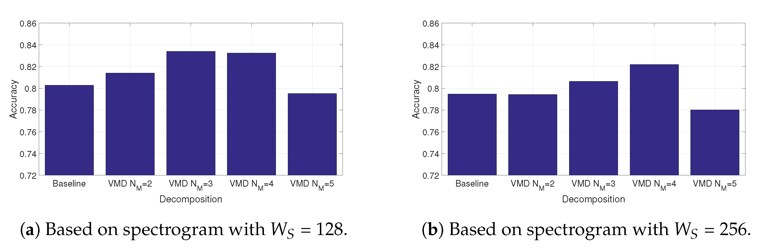
This assumption is validated by the following Figure 4a,b, respectively for spectrograms at $W_S=128$ and $W_S=256$ for different values of $N_M$. Note that these figures are based on a partial application of the approach where the dimensional reduction with LBP is not implemented. Figure 4a,b show that the use of the residual from the VMD is able to outperform the direct application of the DL algorithm on the spectrogram of the original signal for both values $W_S=128$ and $W_S=256$. The potential issue is to select the appropriate value of $N_M$ to achieve the maximum value of the accuracy. For $W_S=128$, the optimal value of $N_M$ is 3 (even if the value of $N_M=4$ achieves a similarly high accuracy). For $W_S=256$, the optimal value of $N_M$ is 4.

In both cases, we notice that a higher value of $N_M=5$ decreases the accuracy.

4.2. Dimensionality Reduction

The previous results were obtained without the application of the dimensionality reduction step. We show with the subsequent results that the use of LBP can reduce the size of the input spectrogram images while preserving the discriminating features and decrease the DL classification time.

To enhance the image content and to place the richest content (from the discriminating point of view) in the center of the figure, a two-sided, centered spectrogram is used instead of the one-sided spectrogram shown in the previous Figure 2b,c.

Figure 5 shows the two-sided centered spectrogram of the original signal with $W_S=256$. The spectrogram was converted to a gray-scale image for the application of LBP.

As described previously, the spectrogram images are split into areas of the same size on which the LBP features are extracted. Each spectrogram image (both the one originating from the baseline and the one originating from the residual after the application of VMD) was divided into 32 areas: 8 divisions along the time domain and 4 divisions along the frequency domain. These subdivisions were executed in this way because of the structure of the LoRa preamble in the time domain (thus a value of 8) and because most of the energy in the centered two-sided spectrogram is along the frequency center line. Then, a value of 8 was used to distinguish between the areas where most of the energy is concentrated and the areas where it is not. A larger number of areas would go against the rationale that on each area the LBP features have to be extracted, which requires a statistically significant number of points to calculate the LBP. In addition to the features generated by LBP (59 in this case), the Shannon entropy of each area is also calculated for a total of 60 features. Then, the DT algorithm was applied to the feature space generated for each area and the resulting accuracy was used to identify the potential areas, which are more promising for the future steps. The DT was used with a maximal number of decision splits equal to 12 and the split criterion with the Gini’s diversity index.

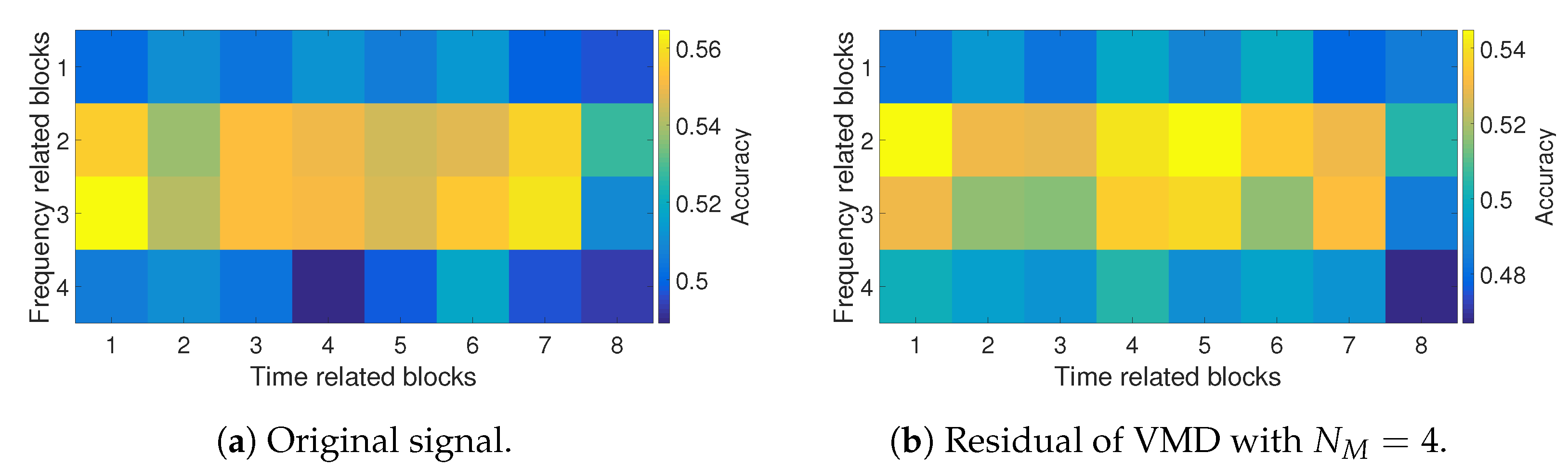
Figure 6a,b below show the accuracy obtained using the LBP, respectively for the spectrogram of the original signal and the spectrogram of the residual using $W_S=128$. The residual was calculated with $N_M$ = 4.

The figures show that the areas with the highest accuracy are along the central frequency region, where most of the energy of the signal is concentrated. Then, the result shown in Figure 6a,b is not surprising, but the proposed approach based on the application of LBP also shows the most promising areas along the time dimension in the central frequency region, which is additional information not provided by the spectral energy density.

Similar results are obtained using $W_S=256$, and they are shown in Figure 7a,b, respectively for the spectrogram of the original signal and the spectrogram of the residual using $N_M$=4. The identification of promising areas is even more evident for $W_S=256$ than for $W_S=128$. In particular, it is shown that the first areas (first along the time dimension) in Figure 7b have significantly higher accuracy than the other areas. This aspect may point to a more effective selection of the areas for $W_S=256$. This assumption will be demonstrated in the subsequent results of this section. It is noted that the accuracy shown in the previous four Figure 6a,b and Figure 7a,b is low in absolute terms (highest values around 55% accuracy), but it is not important in the overall context of the approach because the accuracy is only used to select the most promising areas for further processing by the CNN.

Then, the 8 areas with the highest accuracy over the overall set of 32 areas are selected and assembled to generate reduced images (which are 1/4) of the original size. The 8 areas are selected both for the spectrograms created from the original images and for the spectrogram created from the residuals on the application of VMD. The reduction factor of 4 (8 areas out of 32 areas) is chosen to obtain a significant reduction of the spectrogram images, which can justify the application of the proposed approach as it would decrease the classification time with CNN. As reported in [31], the computational complexity of the CNN convolutional layer is quadratic with the size of the input image. Then, we approximately obtain a $1/16$ reduction of the classification time.

4.3. Detailed Results

Table 2. Detailed results of the proposed approach.

Method	Accuracy	F-Score	Normalized Computation Time
$W_S=128$
Spectrogram of the original signal	0.8028	0.8018	146
Spectrogram of the residual ($N_M=3$)	0.8339	0.8342	199 (63 VMD, 136 CNN)
Reduced spectrogram of the original signal	0.866	0.865	41 (5 Feature, 1 ML, 35 CNN)
Reduced spectrogram of the residual ($N_M=4$)	0.8728	0.8732	104 (63 VMD, 5 Feature, 1 ML, 35 CNN)
$W_S=256$
Spectrogram of the original signal	0.7947	0.7931	150
Spectrogram of the residual ($N_M=4$)	0.8218	0.8202	209 (63 VMD, 146 CNN)
Reduced spectrogram of the original signal	0.907	0.89	41 (5 Feature, 1 ML, 35 CNN)
Reduced spectrogram of the residual ($N_M=4$)	0.919	0.9165	102 (63 VMD, 5 Feature, 1 ML, 33 CNN)

below shows the detailed results for the proposed approach and the baselines (the original signal) for both the window sizes, $W_S$, considered in this study for the obtained accuracy, F-score, and computing time.

Table 2 shows that the proposed approach is able to significantly outperform the application of CNN directly on the original spectrograms as done in [6] for both window sizes, $W_S$. For example, for $W_S=128$ the accuracy obtained using the residual is 0.8339 against the accuracy of 0.8028 obtained using the original signal. The application of the reduction step using LBP significantly increases the accuracy when it is applied to the original signal (accuracy of 0.866) or to the residual (accuracy of 0.8728).

The use of a larger window size (i.e., $W_S=256$) produces even higher accuracy values than the use of $W_S=128$, presumably because a large window size generates a sharper frequency resolution in the spectrogram, which can be exploited by the CNN. In fact, we obtain an accuracy of 0.919 using the reduced spectrogram of the residual and an accuracy of 0.907 using the reduced spectrogram of the original image. The F-score results are usually coherent with the accuracy results.

The total computation time is shown in the last column of Table 2. The time is normalized to the smallest computation time (which is the execution of the DT algorithm on the feature space generated with the application of LBP and Shannon entropy). The computation time is the total of the specific computation times needed for each step in the procedural path chosen in the methodology described in Section 3.1. The computation time of each step is shown in parenthesis after the total in the last column of Table 2. ML identifies the application of the DT algorithm.

It can be noted that the reduction of the images significantly reduces the CNN classification time, which is generally quadratic with the size of the images. The computational time spent on the application of LBP and Shannon entropy is also quite small in comparison to the CNN classification time, and it does not significantly impact the overall computation time. Apart from the CNN classification time, the largest contributor is the execution of the VMD algorithm to all the signals of the data set. The VMD execution is relatively long for this specific data set because each sample is a time series of length 8192 samples and the computing complexity of VMD is related to the size of the time series on which to operate [24]. This is one of the limitations of the proposed approach. Another limitation is that the optimal number of modes is not known a priori.

4.4. Confusion Matrices

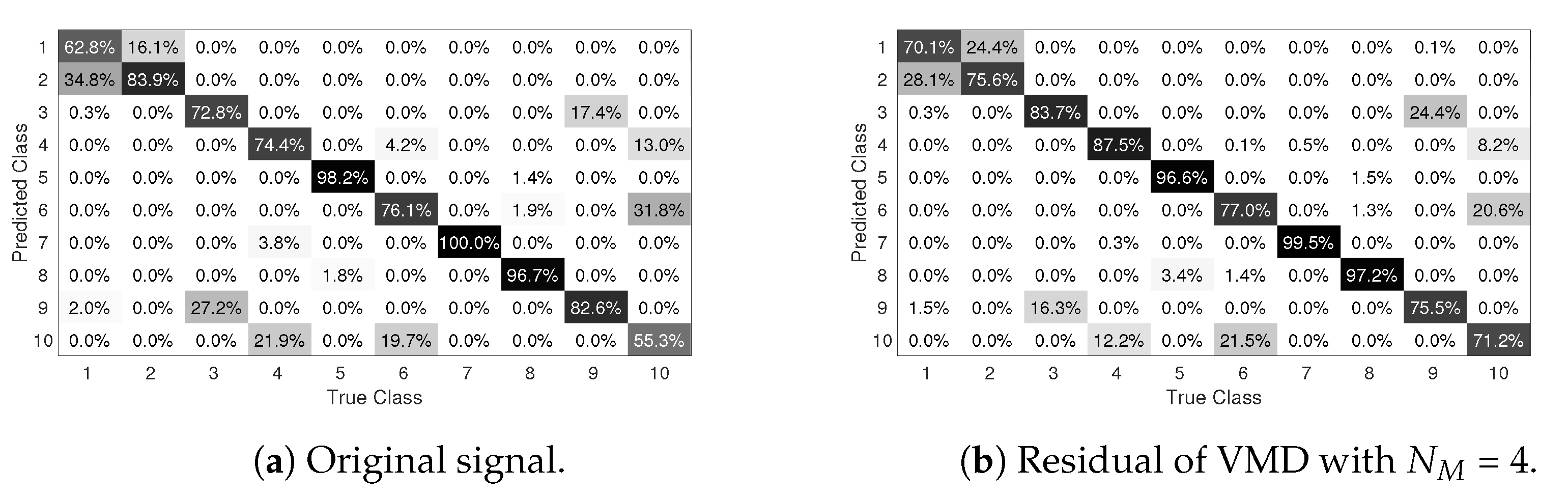
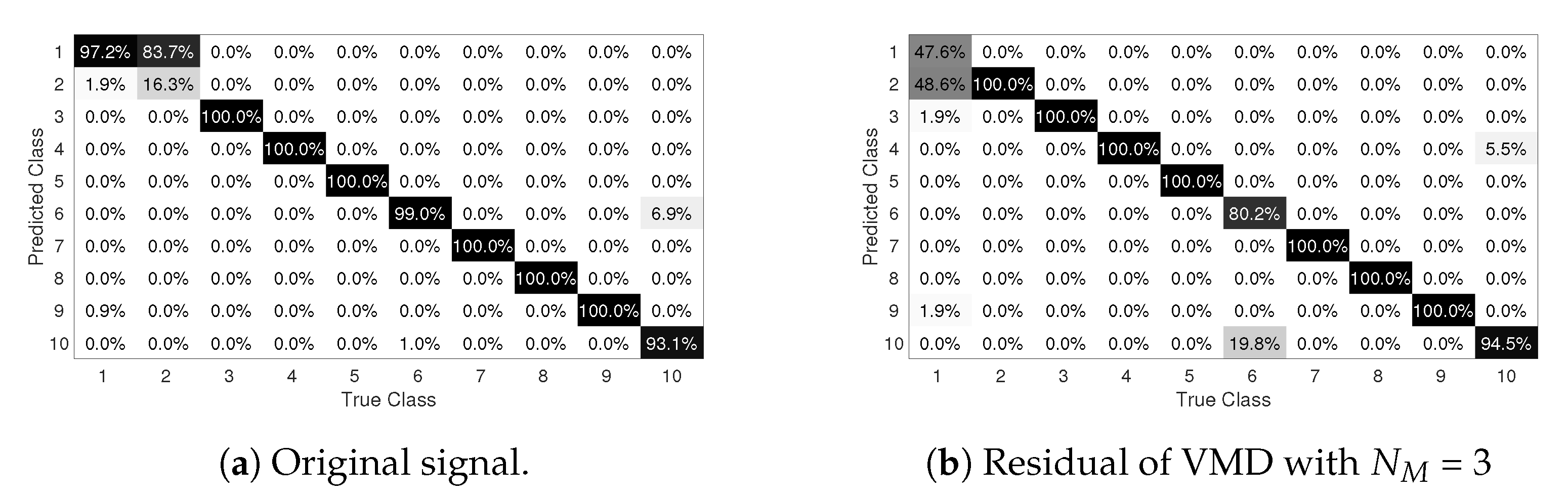
The objective of this sub-section is to provide confusion matrices for specific sets of values of the hyper-parameters $W_S$ and $N_M$ to complement the accuracy results presented in the previous sub-sections. Confusion matrices provide more detailed information in comparison to the overall accuracy as they compare the predicted values against the true values for each wireless emitter.

Figure 8a,b show, respectively, the confusion matrices for the spectrogram calculated with $W_S=128$ and applied to the original signal and the residual after the application of VMD.

Figure 9a,b show, respectively, the confusion matrices for the spectrogram calculated with $W_S=256$ and applied to the original signal and the residual after the application of VMD.

It can be seen that the confusion matrices are aligned with the results presented in Table 2 because the accuracy obtained with $W_S=256$ significantly outperforms the results obtained with $W_S=128$. In particular, the accuracy obtained for specific devices (devices 3, 4, 8, and 9) is 100%, while it can be noted that the first two devices (devices 1 and 2) are more difficult to distinguish. One possible reason for this is that the first two devices have very similar hardware intrinsic features in comparison to the other devices and the classification algorithm has some challenges (i.e., the classification of many samples is wrongly predicted) to distinguish them.

5. Conclusions and Future Developments

This study has proposed a novel approach for RFF, where the VMD is used to highlight the specific differences among the wireless devices (i.e., the fingerprints). The method is based on the extraction of the residuals from the signal generated from the LoRa devices after the application of VMD with a different number of modes. The method is applied to a public data set of 10 LoRa devices, where the preamble is extracted. On the residual signal (and the original signal for comparison), a spectrogram is applied to create images to be given in input to a CNN with a multi-head attention layer. The potential issue with the use of spectrogram is the large size of the image to be fed to the CNN, which may increase the overall classification time. While it is assumed that the CNN will be able to extract the most discriminating features in the images, this proposal uses a dimensionality reduction method, which combines ML and DL. Specifically, the LBP image processing features are used to single out portions of the spectrogram that have the most discriminating power. Therefore, it is a hybrid approach as it combines the computing efficiency of ‘shallow’ ML algorithms with the classification performance of DL. The results show that the proposed approach is able to outperform the baseline approach using the spectrogram on the original signal or even the spectrogram on the residual signal both in terms of classification accuracy and computing time.

The strongest limitation of the proposed approach is the computational time of the application of the VMD, which can be significant, especially for long time series as in this data set. In addition, the optimal number of modes is not known a priori and it must be determined empirically, even if the range of values is limited (from 2 to 4).

Future developments may use other image processing features beyond the LBP or other DL architectures. In addition, more recent mode decomposition algorithms could be used as VMD itself has evolved to more sophisticated algorithms from the initial proposal in [24].