Abstract
To harness the strengths and mitigate the limitations of line-commutated converter (LCC) and modular multilevel converter (MMC) HVDC systems, the LCC-MMC hybrid HVDC system has been developed. This paper proposes a holomorphic embedding (HE)-based power flow calculation method for AC/DC power systems with the LCC-MMC hybrid HVDC system. Firstly, the methodology involves establishing the mathematical model of the LCC-MMC hybrid HVDC system and its control modes. Subsequently, the HE formulation for the constructed LCC-MMC model is derived using the HE method. The proposed method simplifies the HE formulation using substitute variables, making it adaptable to various control modes. The designed HE formulation facilitates the derivation of the germ solution and the calculation of high-order power series coefficients. A sequential solution flow chart compatible with AC power flow algorithms is constructed to enhance the practicality of the HE method for real-world large-scale systems. The accuracy and effectiveness of the proposed method are verified through numerical tests on the modified IEEE 14-bus, IEEE 57-bus, and large 2383-bus system. The proposed method provides a reliable and efficient solution for power flow analysis in hybrid HVDC systems.
1. Introduction
High-voltage direct current (HVDC) transmission system offers significant advantages for efficient and reliable large-scale power transmission in interconnecting power systems. HVDC transmission is suitable for long-distance, large-capacity power transmission and can be applied to interconnecting asynchronous systems, submarine cable transmission, and stable AC systems [1,2,3]. HVDC has been proven to be a preferable solution for addressing the renewable energy integration issue [4].
In HVDC systems, two primary converter technologies are employed: line-commutated converters (LCCs) and voltage-source converters (VSCs). The LCC technology offers advantages such as low losses for long-distance transmission. However, it faces challenges such as commutation failures, harmonics generation, and the need for reactive power compensation and polarity reversal for power flow reversal [5,6,7,8]. On the other hand, VSC technology provides benefits like independent active and reactive power control, improved dynamics, and stable operation without large harmonic filters. However, it incurs higher construction costs, lower power ratings, and typically higher operational losses [9,10,11]. Combining the strengths of LCC and VSC, the hybrid HVDC system presents a promising solution for power transmission with reduced losses and costs, as well as enhanced control flexibility [12,13]. Compared with conventional VSC, a modular multilevel converter (MMC) offers lower voltage harmonics and lower normal operating losses [14]. The hybrid HVDC technology has gained attention in recent years due to several ongoing projects in China, such as the Baihetan–Jiangsu system [15] and the Wudongde–Yunnan system [16].
The study of AC/DC power flow calculation dates back to the 1950s. Since then, extensive research has been conducted to address AC/DC power flow issues in power systems using LCC [17,18,19]. This research has served as a pioneer foundation for subsequent studies on power flow calculations involving various types of converters, such as VSC and current-source converters (CSCs). The unified power flow calculation method was first reported in [20], which described an application for a two-terminal VSC system. Reference [21] introduces a generalized steady-state mathematical model for multi-terminal VSC systems with arbitrary topologies.
The power flow calculation methods for AC/DC systems can be classified into two categories: the unified and the sequential methods. The unified method simultaneously solves the power flow equations of both AC and DC systems, while the sequential method handles them through iteration. The sequential method is convenient to integrate the DC system calculation into existing AC power flow calculation programs with a little modification. Thus, the sequential method is commonly used in the practical EMS for AC/DC power systems [22].
All the methods in the aforementioned reference use the Newton–Raphson (NR) approach to solve the non-linearity of the power flow problem. In practical applications, the NR method may not guarantee fully reliable convergence due to reasons such as unknown convergence regions, potential divergence, and the critical role of initial guess selection, where an inappropriate choice can lead to false solutions [23]. A more robust power flow calculation method should be proposed for steady-state operation evaluations, contingency analysis, and planning for AC/DC systems.
The holomorphic embedding (HE) power flow method introduces a non-iterative approach to power flow analysis [24]. This method reliably yields a power flow solution whenever one exists. Conversely, in scenarios where a solution is non-existent, it issues a collapse signal. The HE method has been used in power flow calculation [25,26,27,28], probabilistic power flow calculation [29], contingency analysis [30,31], voltage stability margin calculation [32,33], dynamic simulation [34], etc. Reference [23] uses HE formulation for LCC-HVDC power flow calculation and obtaining reliable power flow results. Reference [35] utilizes the HE method to solve power flow problems for VSC-HVDC power systems, considering multi-terminal configurations. However, the application of the HE method in LCC-MMC hybrid HVDC systems is currently limited, highlighting the need for the development of the HE method specifically for hybrid HVDC power flow calculations.
This paper proposes an HE-based power flow calculation method for an AC/DC power system that includes LCC-MMC hybrid HVDC. The main contributions of this paper can be summarized as follows:
- (1)
- To the best of our knowledge, this paper is the first to derive the HE formulation for nonlinear power flow equations involving LCC-MMC hybrid HVDC configurations; based on the HE formulation, the germ solution and high-order power series solution process is developed; to circumvent the complexity associated with the trigonometric functions in LCC-MMC equations, this paper introduces substitute variables that simplify the HE formulation; the proposed HE formulation is easy to expand to different control modes; furthermore, the proposed HE formulation is designed to be easily adaptable to various control modes;
- (2)
- To verify the availability of the HE method, the sequential solution flow chart has been constructed; this flow chart can be conveniently compatible with algorithms for AC power flow; this will make the proposed HE method more practical in the real-world large-scale system;
- (3)
- Simulation results demonstrate the effectiveness of the proposed HE method, comparing accuracy and convergence performance compared with the traditional NR method.
This paper is organized as follows: Section 2 introduces the power flow modeling and control modes for the hybrid HVDC system; Section 3 outlines the HE formulation for LCC and MMC stations; in Section 4, we derive the germ solution and high-order power series calculation process, including a flow chart of the sequential power flow solution process for hybrid HVDC; case studies are presented in Section 5, and conclusions are drawn in Section 6.
2. Modelling of Hybrid LCC-MMC HVDC System
The hybrid HVDC system includes both two-terminal and multi-terminal structures. In this paper, we construct the mathematical model for the hybrid two-terminal HVDC system. Figure 1 illustrates the topology of this system, where one terminal employs an LCC converter and the other utilizes an MMC converter [36]. For simplicity, the LCC station is connected to bus i, and the MMC station is connected to bus j. The calculation models for each converter will be elaborated on in subsequent sections.
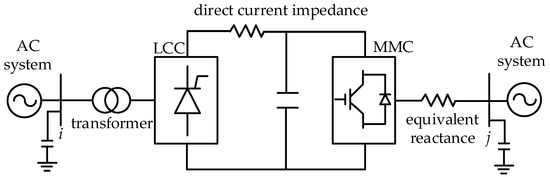
Figure 1.
The topology diagram of the hybrid two-terminal HVDC system.
2.1. The LCC Station Model
The structure of the LCC station is shown in Figure 2 [37].
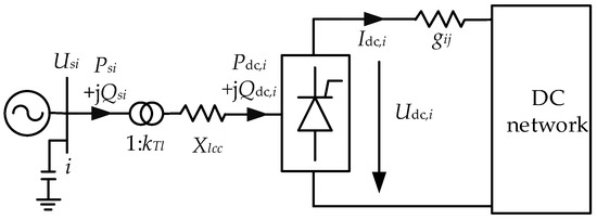
Figure 2.
The diagram for the structure of the LCC station.
In Figure 2, the variables Psi and Qsi denote the active and reactive power injections from the AC side at terminal bus i, respectively; Pdc,i and Qdc,i denote the active and reactive power absorbed by the converter at the DC side, respectively; Usi represents the AC side voltage magnitude at bus i; Xlcc is the equivalent reactance of the converter station; kTl represents the ratio of the converter transformer; Idc,i and Udc,i correspond to the current and voltage at the DC side, respectively. Assuming that the converter losses are negligible, the active and reactive power on both the AC and DC sides of the converter are approximately equal.
The power flow equations for the LCC station are provided by (1)–(3) as follows:
where θi is the converter commutation angle (i.e., rectifier commutation angle or inverter extinct angle); kγ is the parameter obtained by taking into account the commutation effect, usually 0.995; and φi is the converter power factor angle.
The DC network equation for the LCC is shown in (3) as follows:
where nc represents the number of converter stations in the DC network, with nc equalling 2 in the context of the two-terminal HVDC system; gij represents the admittance matrix element of the DC network; and Nj denotes the number of converter bridges at j.
The variables for each LCC station include Udc,i, Idc,i, cosθi, cosφi, and kTl. To ensure that the number of power flow equations matches the number of variables, each LCC station must add two additional equations. This can be achieved by specifying two variables at predetermined values, which are also known as control modes. For the sake of generality, these two equations are not explicitly detailed, as shown in (4)–(5).
For instance, if an LCC station employs constant current control and constant transformer ratio control, (4)–(5) can be explicitly expressed as Δd4 = Idc,i − = 0 and Δd5 = kTl − = 0. Here, and are the predetermined values. The detailed control modes for the LCC station are presented in Section 2.3.
2.2. The MMC Station Model
The MMC is characterized by its lower frequency and reduced losses, and it does not require the addition of a filter. The structure of the MMC station is shown in Figure 3 [38].
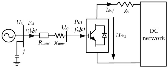
Figure 3.
The diagram for the structure of the MMC station.
In Figure 3, Psj and Qsj represent the active and reactive power injections from the AC side at terminal bus j, respectively; Xmmc denotes the equivalent reactance of the converter; Rmmc represents the equivalent resistance, which is composed of converter losses; Usj represents the voltage magnitude at the AC side at terminal bus j; Ucj represents the voltage of the commutation bridge at the DC side; Udc,j stands for DC side voltage; and Idc,j represents the DC side current.
The power flow equations for the MMC station are presented in (6)–(9) as follows:
where Mj denotes the modulation ratio, with a range from 0 to 1; μd represents the DC voltage utilization, which changes depending on the specific modulation mode used, and is equal to in this paper. The difference in phase angle is given by δj = δsj − δcj. The parameter Yj is defined as Yj =, and βj is calculated as arctan(Xmmc/Rmmc).
The DC network equation for the MMC is shown in (9).
The variables for each MMC station include Udc,j, Idc,j, Mj, δj, Psj, and Qsj. To ensure that the number of power flow equations matches the number of variables, each MMC station must add two additional equations. This can be achieved by specifying two variables at predetermined values, which are also known as control modes. For the sake of generality, these two equations are not explicitly detailed, as shown in (10)–(11).
For instance, if an MMC station employs constant voltage control and constant reactive control, (10)–(11) can be explicitly expressed as Δd10 = Udc,j− = 0 and Δd5 = Qsj − = 0. Here, and are the predetermined values. The detailed control modes for the MMC station are presented in Section 2.3.
2.3. Control Modes
The control modes for the LCC-MMC hybrid HVDC system is different from a pure LCC or pure MMC system. Generally, the sending end adopts the LCC station, and the receiving end adopts the MMC station.
The common control modes for the LCC and MMC stations are presented in Table 1. For the stable operation of the DC network, it is essential to maintain the power balance and the voltage in a normal range. Generally, one end of the converter should be controlled by constant voltage, and the other converter should be controlled by other control modes besides constant voltage control.

Table 1.
LCC and MMC control modes.
Therefore, the hybrid two-terminal HVDC system offers selectable control mode combinations, including either LCC ➀ or ➁ with MMC ➂ or ➃, or LCC ➂ or ➃ with MMC ➀ or ➁.
3. HE Formulation for LCC and MMC Station
The traditional algorithm used for solving the nonlinear equations listed in Section 2 is the NR method. But the convergence of the NR method depends on the selection of initial points and has disadvantages such as poor convergence in ill-conditional situations. To overcome the limitations of the NR method, this section introduces the HE formulation for the LCC and MMC stations.
3.1. HE Method
A holomorphic function is a complex-value analytic function that is infinitely complex differentiable around every point within its domain. The main property of a holomorphic function is that it can be represented by its Taylor series as a function of the complex parameter α [24]. For example, a holomorphic function z(α) can be expressed by the following:
where z[n] denotes the n-th coefficient of the Taylor series expansion.
For nonlinear equations,
If the quantity z to be determined is difficult to solve directly, the HE method constructs a holomorphic function z(α) by embedding a new complex variable α, and embeds it into the original nonlinear equation to form an equation containing a holomorphic function that is as follows:
By performing a Taylor power series expansion on the function z(α), solving its power series coefficient z[n], and substituting it into Equation (12), the implicit function z(α) can be converted into an explicit function with a specific expression. For detailed information on the HE method, readers can refer to [24].
The execution of HE-based power flow calculation involves the following steps:
Step1: Construct HE formulation for all equations;
Step2: Obtain the germ solution;
Step3: Calculate n-th power series coefficients and the target value at α = 1;
Step4: Check convergence; if convergence criterion is met or maximum iteration is reached, go to the next step; otherwise, go to Step 3;
Step 5: Output the power flow calculation results.
In this paper, we design HE formulations for both the LCC station and the MMC station, as well as for various control modes.
3.2. HE Formulation for LCC Station
For each unknown variable, a holomorphic function is constructed using the complex embedding parameter α. For instance, the unknown variable Udc,i is expressed as Udc,i(α). The holomorphic functions for other variables associated with the LCC station are as follows: kTl = kTl(α), Idc,i = Idc,i(α), cosθi = A(α), cosφi = B(α).
The HE formulations for the basic equations of the LCC station are shown in (15)–(16) as follows:
where 2.7 represents the approximate value of . The HE formulation of the DC network equation is presented in (17).
3.3. HE Formulation for MMC Station
Similar to the LCC station, the HE formulation for MMC Equations (6)–(9) has been developed. The variables associated with the MMC station are also represented as holomorphic functions. The holomorphic functions for variables associated with the MMC station are as follows: Psj = Psj(α), Qsj = Qsj(α), Udc,j = Udc,j(α), Mj = Mj(α), cosδi = C(α), sinδi = D(α), Idc,i = Idc,i(α), cosθi = A(α), and cosφi = B(α).
The HE formulation for the power flow equations of the MMC station is presented in (18)–(20).
In (20), the parameter λ can be calculated by the following Equation (21):
where Udc,j[0] Idc,j[0], and Mj[0] are the germ solution and the value can be found in (29)–(40).
The HE formulation for the DC network equation is shown in (22).
To avoid handling trigonometric functions of cos(δj + βj) in (6) and sin(δj + βj) in (7), it is challenging to design the HE formulation directly for δj. Therefore, we use C = cos(δj) and D = sin(δj) as variables to circumvent the need for a direct HE formulation for δj. Once the values of C and D are obtained, we can recover the value of δj. Consequently, an auxiliary equation is introduced, with its corresponding HE formulation presented in (23).
3.4. HE Formulation for Control Modes
As shown in Table 1, there are many different control modes for LCC and MMC stations. In this paper, the LCC station uses constant current and constant transformer ratio control, whereas the MMC station employs constant voltage and reactive power control to validate the proposed method.
The HE formulation for the LCC control mode equations is shown in (24)–(25) as follows:
where and represent the control parameters, specifically the constant current and the constant transformer ratio. Idc0 represents the initial DC current value, which is established by the subsequent guideline. If the LCC station employs constant current control, then Idc0 can be set to . If the LCC station adopts other control modes, Idc0 can be specified with any appropriate value.
The HE formulation for the MMC control mode equations is shown in (26)–(27) as follows:
where and represent the control parameters of the specified MMC, namely DC voltage and reactive power, respectively; Udc0 and Qsj0 denote their initial values, with Udc0 set near the standard unit value and Qsj0 defined as Qsj[0], which can be calculated by (38).
4. Solution Process
The HE formulations for LCC, MMC station, and control modes are shown in (15)–(27). The key solution steps in the HE method for power flow calculation involve obtaining the germ solution and developing a linear equation for high-order power series coefficient calculation. All holomorphic functions in (15)–(27) can be expanded through the summation of power series. Take Udc,i(α) as an example; the summation of power series can be expressed as (28).
4.1. Germ Solution
At α = 0, ensuring that the coefficients on both sides of Equations (15)–(27) are equal yields a germ solution. Given that the HE formulation is specifically designed, it enables the direct derivation of the germ solution, as illustrated in (29)–(40).
4.2. High Order Power Series
The high-order power series coefficients can be obtained by recursively solving the linear equations as shown in (41)–(52), which can be derived by equating the left-hand-side coefficients and right-hand-side coefficients of (15)–(27). The high-order power series coefficients can be obtained from low-order coefficients in a recursive manner, starting from the zeroth-order coefficients known as the germ solution. Equations (41)–(52) are derived individually from the corresponding equations in (15)–(27) as follows:
where E[τ], F[τ], and G[τ], as shown in (47)–(49), are detailed in (53)–(55) as follows:
where δni is the Kronecker delta function, which equals 1 only when the indices i and n are equal, and vanishes for all other orders.
The matrix form of the HE formulation for Equations (41)–(52) is presented in Appendix A, which will help readers understand this process more clearly.
4.3. Flow Chart of the Proposed Method
There are two methodological categories for solving the AC/DC hybrid system: the unified method and the sequential method. In this paper, we employ the sequential method, which solves the AC system and the DC system in sequence.
The exchange of variables between the AC system and the DC system is shown in Figure 4. After the AC power flow calculation, the AC system provides the bus voltage magnitude Usi and Usj to the DC system. Subsequently, the DC system power flow calculation is carried out, and the power injections Psi, Qsi, Psj, and Qsj are transferred to the AC system. Convergence is achieved when the difference in exchanged voltages Usi and Usj between the two systems falls below a specified tolerance.
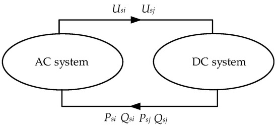
Figure 4.
The exchange of variables between the AC system and the DC system in the sequential method.
The flow chart of the proposed method is illustrated in Figure 5.
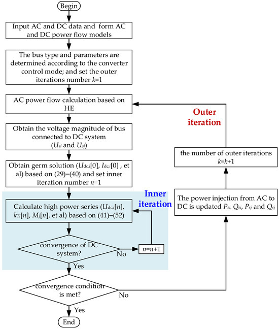
Figure 5.
Flow chart of the sequential power flow solution method for the AC/DC system.
5. Case Study
To verify the effectiveness of the proposed HE-based power flow calculation method for the hybrid HVDC system, tests are carried out using a modified IEEE 14-bus system, a modified IEEE 57-bus system, and a modified 2383-bus system. It is implemented on a laptop with an Intel Core i5-10210U with a 1.60 GHz and 2.11 GHz processor and 24 GB RAM. All original case data are from the MATPOWER toolkit [39]. The convergence criterion for the outer iteration requires that the voltage updates across all buses be less than 1 × 10⁻⁴ p.u. Similarly, the convergence criterion for the inner iteration of the DC system demands that the maximum value of the high-order power series coefficients be less than 1 × 10⁻⁴ p.u.
5.1. Case Introduction
5.1.1. Modified IEEE 14-Bus System
The LCC-MMC HVDC line is embedded between buses 4 and 5. Bus 4 connects to the MMC station and bus 5 connects to the LCC station. Figure 6 shows the diagram of the modified IEEE 14-bus system. The numbers 1–14 in Figure 6 represent the bus numbers in the modified IEEE 14-bus system.
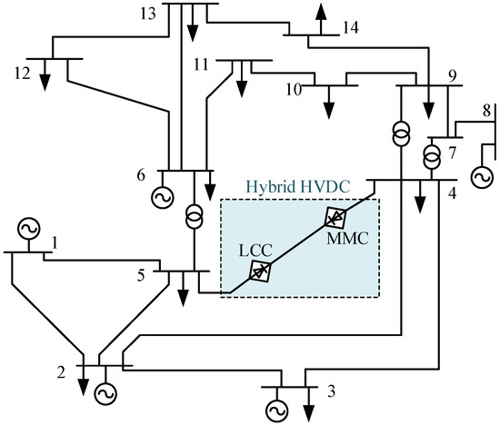
Figure 6.
The diagram of the modified IEEE 14-bus system.
The LCC station uses constant current and constant transformer ratio control, and the MMC station uses constant voltage and constant reactive power control. The control parameters are set as follows: Idc,i = 0.3 p.u., kTl = 1.0 p.u., Udc,j = 2.0 p.u., and Qsj = −0.1 p.u. The rest of the converter parameters are listed in Table 2.
Table 2.
Converter parameters of LCC and MMC stations.
5.1.2. Modified IEEE 57-Bus System
The modified IEEE 57-bus system includes two hybrid LCC-MMC HVDC lines. The diagram of the modified IEEE 57-bus system is shown in Figure 7. The converter parameters for the LCC and MMC stations are also provided in Table 2. The control mode parameters for each converter are listed in Table 3. The numbers 1–57 in Figure 7 represent the bus numbers in the modified IEEE 57-bus system.
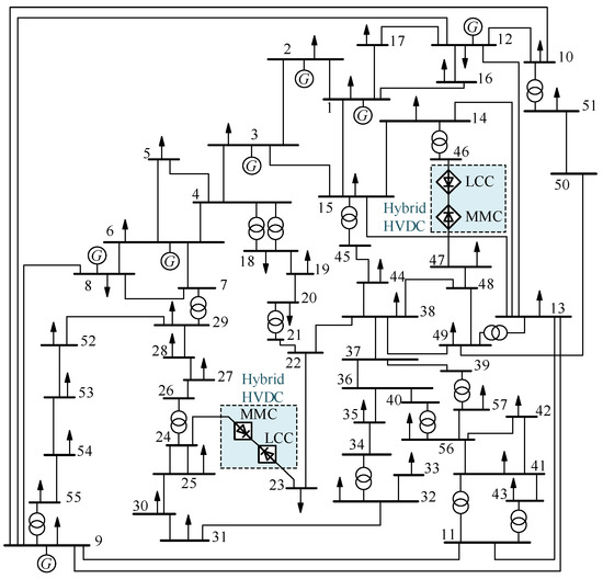
Figure 7.
The diagram of the modified IEEE 57-bus system.
Table 3.
The HVDC line parameters of the modified IEEE 57-bus system.
5.1.3. Modified 2383-Bus System
The modified 2383-bus system includes two hybrid LCC-MMC HVDC lines. The converter parameters for the LCC and MMC stations are also detailed in Table 2. Additionally, the control mode parameters for each converter are presented in Table 4.
Table 4.
The HVDC line parameters of the modified 2383-bus system.
5.2. Simulation Results
5.2.1. Accuracy
The case study is tested on both using the NR method and the HE method. The NR method for the hybrid HVDC system can be found in [1]. The results for the AC system and the DC system are shown in Table 5 and Table 6, respectively.
Table 5.
AC system power flow calculation results of the modified IEEE 14-bus system.
Table 6.
DC system power flow calculation results of the modified IEEE 14-bus system.
As demonstrated in Table 5 and Table 6, the AC system results and DC system results calculated using the proposed HE method are consistent with those obtained via the NR method, verifying the accuracy of the proposed method. The same accuracy results are also shown in the modified IEEE 57-bus system and modified 2383-bus system. Figure 8 shows the voltage magnitude difference between the proposed method and the NR method in the modified IEEE 57-bus system. At all buses, the voltage difference between the two methods is less than 1 × 10⁻⁶, indicating consistent accuracy between the two methods. This consistency is also evident in the modified 2383-bus system. These findings indicate that the proposed method maintains high accuracy across systems of different sizes.
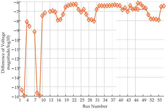
Figure 8.
The difference of voltage magnitude calculated by the HE and NR methods.
5.2.2. Process of Convergence
Figure 9 displays the voltage curve of bus 4 and bus 5 as the outer iteration number k increases. Figure 10 shows the value of the coefficients as the iteration number increases.
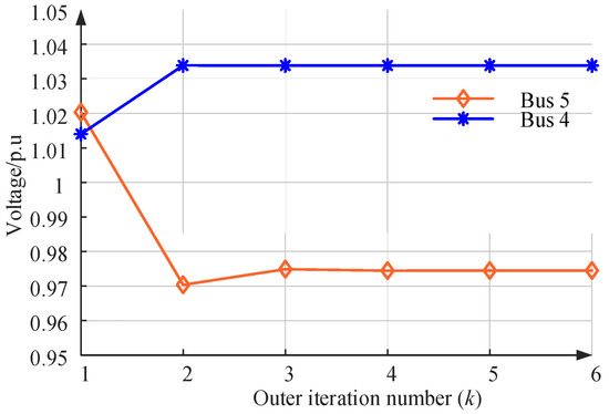
Figure 9.
The voltage in bus 4 and bus 5 with outer iteration number k increasing in the modified IEEE 14-bus system.
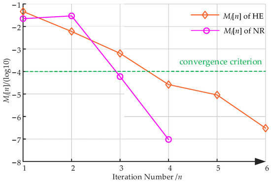
Figure 10.
The coefficients of value Mj[n] with the iteration number n in the outer iteration number k = 1 in the modified IEEE 14-bus system.
As shown in Figure 9, the voltage variables interacting between the AC system and the DC system tend to stabilize after 4 iterations, indicating that the proposed method has converged. Figure 10 displays the values of the coefficients of each order of Mj[n], calculated using both the proposed HE method and the NR method. It can be observed that as the order increases, the high-order coefficient values of Mj[n] decrease rapidly in both methods. The NR method needs three iterations to achieve converge, while the proposed HE method requires four iterations. This indicates that the proposed method can also achieve convergence quickly.
5.2.3. Computational Efficiency
Three modified cases are tested, comparing the HM method proposed in this paper with the NR method in terms of calculation time and outer loop number. The specific results are shown in Table 7.
Table 7.
Time cost of the proposed HE method and NR method.
It can be seen from Table 7 that the outer loop iteration number required by the NR method and the HE method in this paper is the same because the two methods both adopt the sequential solution method. On relatively small-scale systems, IEEE 14-bus and IEEE 57-bus systems, the HE method is slightly slower than the NR method. On the large 2383-bus system, the HE method is faster than the NR method.
The main reason for this is that, in the sequential solution method, whether it is an outer loop or an inner loop, the left-hand-side matrix of the recursive linear equation is a constant coefficient matrix, which does not need to be decomposed again. Meanwhile, when using the NR method, the AC power flow and DC power flow are updated and decomposed in each iteration; specifically, the Jacobian matrix should be updated and decomposed. In the large system, the advantage of the proposed method will be more obvious.
5.2.4. Control Mode Switching
To verify the capability of the proposed HE method in handliing different control mode switches, the control mode of the LCC station at bus number 23 in the modified IEEE 57-bus system will be changed. Initially, the station is under constant current control and constant transformation ratio control. Subsequently, the control mode will be switched to constant current control and constant control angle control, with the control angle set to 0.95.
Before the control mode switch, the voltage magnitude at bus 23 is 0.9335. After switching the control mode to improve the voltage profile, the voltage magnitude increases to 0.9562, indicating an improvement in the voltage profile. Additionally, the transformer ratio of the LCC station is changed from 1 to 0.8261. The voltage magnitude before and after the control mode change is shown in Figure 11.
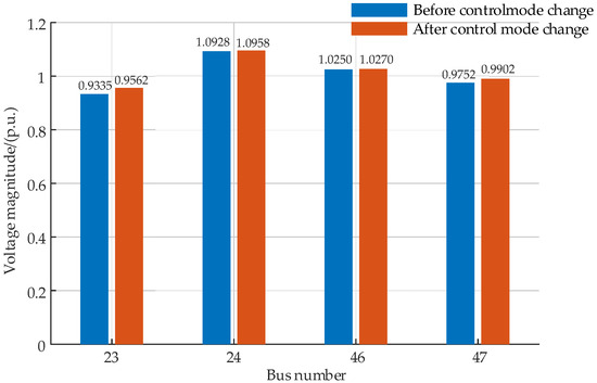
Figure 11.
Comparison of voltage magnitude before and after control mode changes.
These results further validate the flexibility and effectiveness of the proposed method in implementing different control modes.
6. Conclusions
This paper proposes a HE-based power flow calculation method for AC/DC power systems with LCC-MMC hybrid HVDC. The HE formulation for additional nonlinear equations of LCC-MMC is designed. Subsequently, the germ solution and the high-order power series coefficient calculation process are derived. Through tests conducted on the modified IEEE 14-bus, IEEE 57-bus and 2383-bus system, the efficacy of the proposed method is demonstrated by comparing it with the traditional NR method. Compared with the traditional NR method, the HE-based method is theoretically more reliable. The major conclusions can be summarized as follows:
- (1)
- The proposed HE formulation for the LCC-MMC hybrid HVDC system demonstrates practicality and accuracy when compared with the iterative NR method;
- (2)
- In relatively large systems, the proposed method achieves higher computational efficiency compared to the traditional NR method;
- (3)
- The proposed HE formulation can adapt to different control modes, simplifying the calculation process of the germ solution under varying control models;
- (4)
- The sequential method can be implemented with minimal modifications to the existing AC power flow programs, regardless of whether using the NR or HE method; as a result, the sequential method may be more widely accepted due to practical considerations and computational costs.
The work carried out in this paper provides guidance for further research on power flow calculation based on the HE method in AC/DC systems. The proposed method has the potential to be extended to systems with multi-terminal the LCC-MMC hybrid HVDC system in future work. In new-type power systems, power flow calculations are integral to tasks such as static security analysis, power system optimal planning, probabilistic power flow calculation, and other critical functions. Furthermore, the significance of online assessment software is expected to grow, particularly in safeguarding high renewable energy-integrated power systems. Consequently, there is an urgent demand for a power flow algorithm that is both fast and reliable. Compared to traditional iterative methods, the HE method demonstrates considerable advantages in addressing these needs.
Author Contributions
Conceptualization, Y.L. and C.L.; methodology, Y.L. and Z.H.; software, Y.L. and Z.H.; validation, C.L., Z.H. and Y.L.; formal analysis, C.L., Z.H. and Y.L.; investigation, Y.L. and Z.H.; resources, C.L. and Y.J.; writing—original draft preparation, Y.L. and Z.H. writing—review and editing, C.L., Q.C. and Y.L.; supervision, C.L. All authors have read and agreed to the published version of the manuscript.
Funding
This research was supported by the National Natural Science Foundation of China under Project 52007133.
Data Availability Statement
All data used to support the findings of this study are included within the article.
Conflicts of Interest
The authors declare no conflicts of interest.
Appendix A
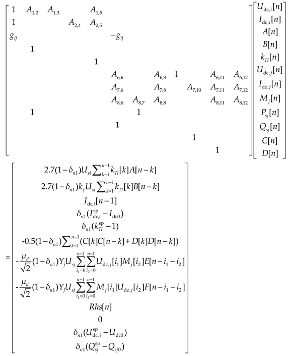
The matrix form of Equations (41)–(52) for the calculation of high-order power series coefficients is given by (A1) as follows:
 , , , , , , , , , , , , , , , , , .
where Rhs[n] is expressed as in (A2) as follows:
References
- Lei, J.; An, T.; Du, Z.; Yuan, Z. A General Unified AC/DC Power Flow Algorithm with MTDC. IEEE Trans. Power Syst. 2017, 32, 2837–2846. [Google Scholar] [CrossRef]
- Li, Q.; Zhao, N. General Power Flow Calculation for Multi-Terminal HVDC System Based on Sensitivity Analysis and Extended AC Grid. IEEE Trans. Sustain. Energy 2022, 13, 1886–1899. [Google Scholar] [CrossRef]
- Nami, A.; Liang, J.; Dijkhuizen, F.; Demetriades, G.D. Modular Multilevel Converters for HVDC Applications: Review on Converter Cells and Functionalities. IEEE Trans. Power Electron. 2015, 30, 18–36. [Google Scholar] [CrossRef]
- Benato, R.; Gardan, G. A Novel AC/DC Power Flow: HVDC-LCC/VSC Inclusion Into the PFPD Bus Admittance Matrix. IEEE Access 2022, 10, 38123–38136. [Google Scholar] [CrossRef]
- Wang, G.-D.; Wai, R.-J.; Liao, Y. Design of Backstepping Power Control for Grid-Side Converter of Voltage Source Converter-Based High Voltage DC Wind Power Generation System. IET Renew. Power Gener. 2013, 7, 118–133. [Google Scholar] [CrossRef]
- Martínez-Parrales, R.; Fuerte-Esquivel, C.R.; Alcaide-Moreno, B.A.; Acha, E. A VSC-based Model for Power Flow Assessment of Multi-terminal VSC-HVDC Transmission Systems. J. Mod. Power Syst. Clean Energy 2021, 9, 1363–1374. [Google Scholar] [CrossRef]
- Wang, S.; Gao, S.; Chen, Z.; Zhao, X.; Song, T.E.; Liu, Y.; Yu, D.; Jiang, S. Analysis of the Operating Margin Evaluation of Multi-Infeed LCC-HVDC Systems Based on the Equivalent Impedance. IEEE Access 2021, 9, 66268–66281. [Google Scholar] [CrossRef]
- Gnanarathna, U.N.; Gole, A.M.; Jayasinghe, R.P. Efficient Modeling of Modular Multilevel HVDC Converters (MMC) on Electromagnetic Transient Simulation Programs. IEEE Trans. Power Deliv. 2011, 26, 316–324. [Google Scholar] [CrossRef]
- Prieto-Araujo, E.; Bianchi, F.D.; Junyent-Ferre, A.; Gomis-Bellmunt, O. Methodology for Droop Control Dynamic Analysis of Multiterminal VSC-HVDC Grids for Offshore Wind Farms. IEEE Trans. Power Deliv. 2011, 26, 2476–2485. [Google Scholar] [CrossRef]
- Lan, T.; Sun, H.; Zhong, W.; Jing, Y.; Zhao, B.; Xu, J. LCC-HVDC’s Systematical Impact on Voltage Stability: Theoretical Analysis and a Practical Case Study. IEEE Trans. Power Syst. 2023, 38, 1663–1675. [Google Scholar] [CrossRef]
- Zhang, L.; Harnefors, L.; Nee, H.-P. Modeling and Control of VSC-HVDC Links Connected to Island Systems. IEEE Trans. Power Syst. 2011, 26, 783–793. [Google Scholar] [CrossRef]
- Flourentzou, N.; Agelidis, V.G.; Demetriades, G.D. VSC-Based HVDC Power Transmission Systems: An Overview. IEEE Trans. Power Electron. 2009, 24, 592–602. [Google Scholar] [CrossRef]
- Torres-Olguin, R.E.; Molinas, M.; Undeland, T. Offshore Wind Farm Grid Integration by VSC Technology with LCC-Based HVDC Transmission. IEEE Trans. Sustain. Energy 2012, 3, 899–907. [Google Scholar] [CrossRef]
- Hu, J.; Xu, K.; Lin, L.; Zeng, R. Analysis and Enhanced Control of Hybrid-MMC-Based HVDC Systems During Asymmetrical DC Voltage Faults. IEEE Trans. Power Deliv. 2017, 32, 1394–1403. [Google Scholar] [CrossRef]
- Li, Z.; Zhan, R.; Li, Y.; He, Y.; Hou, J.; Zhao, X.; Zhang, X.P. Recent developments in HVDC transmission systems to support renewable energy integration. Glob. Energy Interconnect. 2018, 1, 595–607. [Google Scholar]
- Lee, G.-S.; Kwon, D.-H.; Kim, Y.-K.; Moon, S.-I. A New Communication-Free Grid Frequency and AC Voltage Control of Hybrid LCC-VSC-HVDC Systems for Offshore Wind Farm Integration. IEEE Trans. Power Syst. 2023, 38, 1309–1321. [Google Scholar] [CrossRef]
- Smed, T.; Andersson, G.; Sheble, G.B.; Grigsby, L.L. A New Approach to AC/DC Power Flow. IEEE Trans. Power Syst. 1991, 6, 1238–1244. [Google Scholar] [CrossRef]
- Braunagel, D.A.; Kraft, L.A.; Whysong, J. Inclusion of DC Converter and Transmission Equation Directly in Newton Power Flow. IEEE Trans. Appar. Syst. 1976, 95, 76–88. [Google Scholar] [CrossRef]
- Arrillaga, J.; Smith, B. The Power Flow Solution. In AC-DC Power System Analysis; Institution of Engineering and Technology: London, UK, 1998; pp. 78–86. [Google Scholar]
- Zhang, X. Multiterminal Voltage-Sourced Converter-Based HVDC Models for Power Flow Analysis. IEEE Trans. Power Syst. 2004, 19, 1877–1884. [Google Scholar] [CrossRef]
- Beerten, J.; Cole, S.; Belmans, R. Generalized Steady-State VSC MTDC Model for Sequential AC/DC Power Flow Algorithms. IEEE Trans. Power Syst. 2012, 27, 821–829. [Google Scholar] [CrossRef]
- Liu, C.; Zhang, B.; Hou, Y.; Wu, F.F.; Liu, Y. An Improved Approach for AC-DC Power Flow Calculation with Multi-Infeed DC Systems. IEEE Trans. Power Syst. 2011, 26, 862–869. [Google Scholar] [CrossRef]
- Zhao, Y.; Li, C.; Ding, T.; Hao, Z.; Li, F. Holomorphic Embedding Power Flow for AC/DC Hybrid Power Systems Using Bauer’s Eta Algorithm. IEEE Trans. Power Syst. 2021, 36, 3595–3606. [Google Scholar] [CrossRef]
- Trias, A. The Holomorphic Embedding Load Flow Method. In Proceedings of the 2012 IEEE Power and Energy Society General Meeting, San Diego, CA, USA, 22–26 July 2012; pp. 1–8. [Google Scholar]
- Luo, Y.; Liu, C. Area Interchange Control Using the Holomorphic Embedding Load Flow Method Considering Automatic Generation Control. Electr. Power Syst. Res. 2023, 225, 109721. [Google Scholar] [CrossRef]
- Sur, U.; Biswas, A.; Bera, J.N.; Sarkar, G. Holomorphic Embedding Power Flow Analysis of Hybrid-Tidal-Farm-Integrated Power Distribution System. IEEE Syst. J. 2022, 16, 2277–2288. [Google Scholar] [CrossRef]
- Freitas, F.D.; Santos, A.; Fernandes, L.; Acle, Y. Restarted Holomorphic Embedding Load-Flow Model Based on Low-order Padé Approximant and Estimated Bus Power Injection. Int. J. Electr. Power Energy Syst. 2019, 112, 326–338. [Google Scholar] [CrossRef]
- Rao, S.; Feng, Y.; Tylavsky, D.J.; Subramanian, M.K. The Holomorphic Embedding Method Applied to the Power-Flow Problem. IEEE Trans. Power Syst. 2016, 31, 3816–3828. [Google Scholar] [CrossRef]
- Liu, C.; Sun, K.; Wang, B.; Ju, W. Probabilistic Power Flow Analysis Using Multi-Dimensional Holomorphic Embedding and Generalized Cumulants. IEEE Trans. Power Syst. 2018, 33, 7132–7142. [Google Scholar] [CrossRef]
- Wang, Q.; Lin, S.; Gooi, H.; Yang, Y.; Liu, W.; Liu, M. Calculation of Static Voltage Stability Margin Under N-1 Contingency Based on Holomorphic Embedding and Pade Approximation Methods. Int. J. Elect. Power Energy Syst. 2022, 142, 108358. [Google Scholar] [CrossRef]
- Yao, R.; Qiu, F.; Sun, K. Contingency Analysis Based on Partitioned and Parallel Holomorphic Embedding. IEEE Trans. Power Syst. 2022, 37, 565–575. [Google Scholar] [CrossRef]
- Wang, B.; Liu, C.; Sun, K. Multi-Stage Holomorphic Embedding Method for Calculating the Power-Voltage Curve. IEEE Trans. Power Syst. 2018, 33, 1127–1129. [Google Scholar] [CrossRef]
- Rao, S.; Tylavsky, D.; Feng, Y. Estimating the Saddle-Node Bifurcation Point of Static Power Systems Using the Holomorphic Embedding Method. Int. J. Elect. Power Energy Syst. 2017, 84, 1–12. [Google Scholar] [CrossRef]
- Yao, R.; Sun, K.; Shi, D.; Zhang, X. Voltage Stability Analysis of Power Systems with Induction Motors Based on Holomorphic Embedding. IEEE Trans. Power Syst. 2019, 34, 1278–1288. [Google Scholar] [CrossRef]
- Huang, Y.; Ai, X.; Fang, J.; Yao, W.; Wen, J. Holomorphic Embedding Approach for VSC-based AC/DC Power Flow. IET Gener. Transm. Distrib. 2020, 14, 6239–6249. [Google Scholar] [CrossRef]
- Xiong, Y.; Li, F.; Xu, P.; Zhang, C.; Cao, Z. Research on Power Flow Algorithm of LCC and VSC Hybrid Multi-Terminal AC-DC System. In Proceedings of the 2018 2nd IEEE Conference on Energy Internet and Energy System Integration (EI2), Beijing, China, 20–22 October 2018; pp. 1–6. [Google Scholar]
- Shu, T.; Lin, X.; Peng, S.; Du, X.; Chen, H.; Li, F.; Tang, J.; Li, W. Probabilistic Power Flow Analysis for Hybrid HVAC and LCC-VSC HVDC System. IEEE Access 2019, 7, 142038–142052. [Google Scholar] [CrossRef]
- Song, Z.; Huang, Y.; Zhao, H.; Xu, J.; Zhao, C.; Jia, X. Power Flow Calculation Method of AC/DC System with LCC-MMC Series/Parallel Hybrid HVDC. Power Syst. Technol. 2023, 47, 2860–2868. [Google Scholar]
- Zimmerman, R.D.; Murillo-Sánchez, C.E.; Thomas, R.J. MATPOWER: Steady-State Operations, Planning, and Analysis Tools for Power Systems Research and Education. IEEE Trans. Power Syst. 2011, 26, 12–19. [Google Scholar] [CrossRef]
Disclaimer/Publisher’s Note: The statements, opinions and data contained in all publications are solely those of the individual author(s) and contributor(s) and not of MDPI and/or the editor(s). MDPI and/or the editor(s) disclaim responsibility for any injury to people or property resulting from any ideas, methods, instructions or products referred to in the content. |
© 2024 by the authors. Licensee MDPI, Basel, Switzerland. This article is an open access article distributed under the terms and conditions of the Creative Commons Attribution (CC BY) license (https://creativecommons.org/licenses/by/4.0/).