Abstract
Indoor Positioning Systems (IPSs) have multiple applications. For example, they can be used to guide people, to locate items in a warehouse and to support the navigation of Automated Guided Vehicles (AGV). Currently most AGVs use local pre-defined navigation systems, but they lack a global localisation system. Integrating both systems is uncommon due to the inherent challenge in balancing accuracy with coverage. Visible Light Position (VLP) offers accurate and fast localisation, but it encounters scalability limitations. To overcome this, this paper presents a novel Image Sensor-based VLP (IS-VLP) identification method that harnesses existing Light Emitting Diode (LED) lighting infrastructure to substitute both navigation and localisation systems effectively in the whole area. We developed an IPS that achieves six-axis positioning at 90 Hz refresh rate using OpenCV’s solvePnP algorithm and embedded computing. This IPS has been validated in a laboratory environment and successfully deployed in a real factory to position an operative AGV. The system has resulted in accuracies better than 12 cm for 95% of the measurements. This work advances towards positioning VLP as an appealing choice for IPS in industrial environments, offering an inexpensive, scalable, accurate and robust solution.
1. Introduction
The rise of Industry 4.0 has mobilised the scientific community to investigate and develop several positioning systems that would work in indoor environments, where the availability and precision of Global Navigation Satellite Systems (GNSS) is insufficient. Indoor environments pose more challenging requirements: where the 3 m accuracy provided globally by GNSS could mean an Automated Guided Vehicle (AGV) drifting out of its secure path, the localisation of a person in a wrong room during an emergency rescue or the localisation of an asset in a wrong shelf inside of a warehouse.
An Indoor Positioning System (IPS) is usually characterised by the magnitude of its accuracy, ranging from metres to centimetres, and the coverage that it offers, ranging from hundreds of metres to centimetres. Most of the time, balancing these two factors is problematic, as better accuracy is usually associated with worse coverage. Additionally, if the IPS is intended for mobile objects, the positioning rate and the latency of the system become critical, especially for collision avoidance or navigation purposes. Finally, an affordable positioning solution may consider not only the cost of the hardware per se, but also its energy efficiency (to foresee the needs of batteries) and its scalability (in terms of both infrastructure cost and the system’s capabilities). These criteria align with the features evaluated by [1,2].
Our motivation in this work is to explore an IPS solution that can be appealing to a factory environment, focusing on reducing the costs of deployment and maintenance. We envision a scalable system that (1) uses inexpensive hardware in both the transceiver and receiver sides, (2) minimises and facilitates the deployment of infrastructure, (3) achieves centimetre-level positioning, (4) offers a reasonable ratio of coverage per device and (5) provides an acceptable real-time positioning rate [3].
Autonomous guided vehicles, depending on the different requirements of factories, usually rely on two independent positioning systems: one dedicated to navigating around the factory and another to localise assets or perform precise operations, such as cargo loading or manoeuvring around corners. The costs of deploying these IPSs increases proportionally to the factory size, as the spots where high precision is required also increase. Therefore, a system able to provide navigation and accurate localisation would be highly desirable.
An essential feature of AGVs is the concept of “alert zones”. These zones represent a specific volume surrounding the robot where the vehicle can quickly detect obstacles through dedicated sensors. The size of this alert zone depends on the speed of the AGV and the accuracy of its positioning system. When an object is recognised within the alert zone, it triggers actions to prevent collisions. Typically, these actions involve reducing the AGV’s speed or completely stopping it. This crucial feature ensures the safety of AGVs as they drive. The size of this alert zone can also be determinant to define whether a path is traversable by the AGV. For example, a centimetre-level IPS would allow two AGVs to drive side by side in a road that has not been initially designed for that purpose, or it could be used to simply design narrower lanes for the AGV, freeing the space for other more profitable purposes.
The authors in [3] studied positioning requirements for autonomous vehicles in an outdoor environment. They stated that the characteristics of the road and the dimensions of the vehicle are the most relevant factors when determining how much accuracy is needed in the positioning of the vehicle. They also defined that the positioning frequency should guarantee that the distance travelled between two consecutive positioning updates is smaller than 10% of the positioning accuracy required for that road. They concluded that a minimum frequency of 100 Hz is sufficient for both highway and local street operations in the United States of America. By extension, fulfilling this requirement would also make a solution suitable for indoor operation. Given the typical position update rates of standard positioning technologies such as GNSS (1 to 10 Hz) or Light Detection and Ranging (LIDAR) (10 to 30 Hz), achieving a minimum frequency of 100 Hz would be challenging. For this reason, these solutions can be combined with Inertial Measurement Units (IMU) to achieve an acceptable update rate using dead reckoning. Though it is clear that sensor fusion systems can help to improve the performance and can provide redundancy to existent IPSs, in this research we pretend to explore the development of a standalone positioning system capable to meet realistic indoor positioning requirements for industry scenarios.
In this work, we developed a real-time solution for positioning that uses Image Sensor Visible Light Positioning (IS-VLP) technology together with a novel identification method that uses the variation in a light dazzle, instead of the rolling shutter and light-coding scheme. This leads to improvements in scalability and flexibility. This solution was implemented using a Linux-based, low-budget prototyping board, a pinhole camera with fisheye lens and Commercial Off-the-Shelf (COTS) light bulbs. The system can estimate a new position 90 times per second. It is also robust to different lighting environments and is adaptable to different deployment characteristics (light arrangement, distance between lights and height of the lights). We tested this solution in a laboratory environment as well as in a factory environment, where we attached the device to an operating AGV and recorded 138 trajectories during a span of 16 days.
The remainder of this paper is organised as follows. Section 2 reviews the main IPS technologies. Section 3 provides contextualisation, reasoning and a detailed description of the proposed novel method of identification. Section 4 introduces the selected hardware components for implementing the positioning solution. Section 5 focuses on the explanation of the developed software for image processing and position calculation, and Section 6 explains the configuration of the two testbeds used to validate the solution. Section 7 details the data analysis methods and objectives, while Section 8 presents the results for the tests conducted in both laboratory and factory scenarios. Section 9 interprets the results and discusses the main findings. Finally, Section 10 summarises the contributions, offers insights into future work and concludes our research.
2. State of the Art
Some of the most popular standalone indoor positioning systems that use Radio Frequency (RF) rely on the deployment of an on-purpose infrastructure, such as Ultra-Wideband (UWB), Bluetooth/Bluetooth Low Energy (BT/BLE) and Zigbee and Radio Frequency Identification (RFID). A performance comparison of these technologies can be found in [4]. These solutions must overcome the cost of deploying such infrastructure and coexist with other radio frequencies in some of the environments. Other positioning systems rely on algorithms that perform Simultaneous Localisation and Mapping (SLAM) using laser, ultrasounds or images, which do not need an on-purpose infrastructure. However, they become dependent on environment changes, and these are usually complex and costly systems [5]. Lastly, some systems attempt to use existent infrastructure to position, such as Wi-Fi or VLP. While Wi-Fi seems a good candidate that overcomes the Line-Of-Sight (LOS) constraint of VLP, the system would require the deployment of additional/on-purpose Access Points (APs) to achieve an acceptable accuracy [6].
The authors in [6] compare 12 indoor positioning systems for mobile robots, where VLP ranked fourth on accuracy after LIDAR, Ultrasounds (US) and RFID positioning. Although ranked slightly worse on accuracy, Computer Vision (CV) and UWB positioning can be considered relevant because they have a notable coverage capability.
From these technologies, the most appealing positioning systems for businesses would be those that are infrastructureless, which would be US, LIDAR and CV. US and LIDAR technology share the same working principle but differ in hardware cost (LIDAR options are significantly more expensive), and also in the operative range, which is significantly smaller for the US solutions. LIDAR weaknesses are spacious environments (sometimes needing additional reflectors in places where the structural elements such as walls are too far away) and its processing complexity, which would be difficult to execute on affordable hardware. CV is still far from reaching a precise positioning system that uses inexpensive hardware. Moreover, its processing complexity makes it difficult to achieve frequent updates without the support of an edge computing device.
The remaining positioning solutions (VLP, UWB and RFID) rely on an on-purpose infrastructure. While VLP does not face radio spectrum interference issues, its main drawback is the LOS restrictions, especially when considering the coverage of the solution. RFID’s low operating range requires a bigger deployment of infrastructure in order to provide a positioning accuracy comparable to the other technologies. Finally, UWB offers good coverage and decent accuracy, and it is gaining rapid adoption in the Smartphone market, boosting the number of applications and use cases for this technology. However, UWB’s achievable accuracy depends on the environment where it is deployed, as it must address challenges such as multipath interference and Non-Line of Sight (NLOS) conditions.
Light Emitting Diode (LED) lighting advantages over other artificial light sources are widely agreed upon and we see the transformation of all other lighting systems towards it, enforced by the end of EU’s exception towards fluorescent lamps in their Restriction of Hazard Substances Directive [7], which forbids the production of fluorescent lamps in the EU as of September 2023. Soon, more people will profit from LED lighting’s ability to oscillate at high frequencies to both illuminate and transmit information. We believe that using VLP devices that employ already existing LED lighting and provide precise navigation in an industrial environment is an interesting approach to minimising the costs of deployment of such an infrastructure and, at the same time, enabling the possibility to foster its communication and privacy capabilities for other use cases [1].
In VLP, researchers have explored positioning using photodiodes (PD-VLP) as the capturing sensor. However, many of these solutions heavily rely on factors related to the lighting infrastructure, including the need to determine the exact intensity of the LEDs, to achieve precise time synchronisation between the sensor and the LEDs, or to utilise arrays of photodiodes [8]. For this reason, most of the recent research around VLP focuses on using image sensors as the capturing sensor (which most often means using Complementary Metal-Oxide Semiconductor (CMOS) cameras). These approaches can apply computer vision techniques to use fainter signals, discard interferences or detect geometrical patterns.
In VLP, the first step to provide positioning is to identify the lights in view and to discover their 3D coordinates. Most of the work conducted around IS-VLP makes use of a line-coding scheme, produced by the camera’s rolling shutter in combination with high frequency On–Off Keying (OOK) of the LED. The authors in [9] were one of the first to use this method, and since then it has been used as visual landmarks for positioning in several implementations [10,11,12,13]. However, to accurately determine the thickness in pixels of the generated bars, and, consequently, to identify the light, it is necessary to use higher resolutions, which imply a longer processing time. The line-coding scheme also has an important limitation on how far the source light can be detected. The authors in [10,12] show that the decoding rate decays quickly when increasing the distance from the camera to the LED, not being able to decode at 3 m.
Moreover, an important flaw in the line-coding system is the limitation on the number of lights that can be uniquely identified using the rolling shutter effect of a CMOS camera. The resolution of the camera, the speed of the vehicle, the distance to the light and the size of the light are limiting factors for the maximum number of bits that can be transmitted, and, thus, for the number of different identifiers that can be encoded. For example, the authors in [12,14,15] achieve a bit rate of 45, 60 and 100 bps, respectively, at a distance of 2 m and in static conditions. This implies that in 100 ms they would be able to communicate 4, 6 and 10 bits that could be used to encode at most 16, 64 and 1024 different identifiers, respectively. This weakness can be bypassed by adding complexity on the application layer, such as the information of IMUs or BLE beacons. The additional hardware can communicate spatial information to unequivocally identify the lights. The additional hardware can provide spatial information to unequivocally identify the lights.
The variety of algorithms to determine the position in the IS-VLP system is wide, but the function solvePnP included in the Open Computer Vision (OpenCV) library [16] stands out because it provides positioning on six degrees of freedom by using references in any geometric distribution. In contrast to the custom algorithms presented in [17,18], the use of this solvePnP presents some limitations in terms of the number of minimum references necessary to obtain a position, needing either four references at the same height (or plane), or six references. However, as it is a tool with good support and it is easy to use, it is becoming a preferred option for obtaining positions in 3D from a 2D image [19,20,21,22,23].
One of the problems associated with indoor positioning systems is the deployment and setup of the infrastructure. In most cases, it requires conducting many measurements, which must be as precise as possible since the accuracy of the system will depend on it. As demonstrated in [24], a measurement error in the position of the lights is magnified eight times in the position estimated by solvePnP. Overcoming this threat in large deployments becomes increasingly difficult and costly. The approach presented in [25] could help to resolve this limitation for large-scale deployments.
Most of the published research on novel IPS solutions does not provide experimental results in operational factories due to the challenges of engaging the industrial sector. The authors in [26,27] successfully deployed IPS using Wi-Fi and UWB infrastructure in an unmodified factory environment. These deployments covered large areas of the factory, circa 6000 and 60 m2, but they achieved accuracies of less than 6 m and less than 1 m, respectively. This underscores the difficulty in balancing coverage and accuracy.
Current commercial robot solutions for the industrial or service sector, such as the PuduBot 2 from Pudu Robotics, offer similar performance to the work presented in this article in terms of positioning performance [28]. Both approaches use a camera pointing to the ceiling, but the PuduBot 2 approach is different as it is based on Video-SLAM (VSLAM). It is an interesting approach, but the use of VSLAM is sensitive to changes in the environment and requires a learning stage.
3. IS-VLP-Based Novel Identification Method
This work proposes to use the flickering frequency of an LED source as the method for identifying lights by detecting the variation in the captured light beam (dazzle) with a CMOS camera. To illustrate the dazzle variation, Figure 1 shows two consecutive frames captured by the camera pointing to a ceiling with eight light bulbs flickering at different frequencies (delimited by the blue box). The other illuminated areas correspond to potential interferences that the system should be able to distinguish and filter. Comparing both frames, the difference in intensity in each bulb is clearly visible. Instead of measuring the intensity of each dazzle, we decided to measure the illuminated area in pixels, which performs better in terms of computing efficiency and reliability.
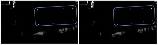
Figure 1.
Consecutive grey-scale frames (11 ms difference) captured by the camera in the factory environment, illustrating the intensity variation in the VLP light bulbs (delimited by the blue box) and the presence of external interferences (factory skylights).
Monitoring the variation in the dazzle is an effective method to identify the flickering frequency of each light. However, identifying lights by frequencies implies that the number of possible identifiers is limited by the number of frequencies that can be detected using a camera. The number of detectable frequencies depends on the image acquisition rate (or frame rate) and the duration of the video (specifically its inverse—the frequency resolution). Most of the inexpensive CMOS cameras cannot achieve a high frame rate, usually ranging from 15 to 90 frames per second, depending on the image resolution.
To work at frequencies that are identifiable by those cameras, the lights would need to flicker between 0 and 50 Hz (based on the Nyquist–Shannon sampling theorem), which would not be feasible as the flicker would be directly noticeable by most human eyes [29]. To overcome this problem, we use an undersampling technique that enables the use of flickering frequencies above the sampling frequency of the cameras, over 100 Hz, which are directly unnoticeable by the human eye.
However, as [30] remarks, flickering lighting can be indirectly noticeable due to the stroboscopic effect, especially for frequencies below 1 kHz in a dimly lit environment. To quantify this effect, the authors in [29] proposed the Stroboscopic Visibility Measure (SVM), a metric that allows for estimating the visibility of the stroboscopic effect created by a flickering light, based on the variation in its illuminance, and adjusted to human sensitivity. The SVM relies on experimental studies and a value of 1 means that 50% of the people exposed to the flickering light would be able to perceive a stroboscopic effect. The European Union has established a precautionary limit at 0.4 [31], despite insufficient data to support this limitation [32].
In the frequency analysis on an undersampled signal, the original frequency will appear as an alias inside a range from 0 Hz to the Nyquist frequency (FN), which is half of the sampling frequency (Fs). The frequency domain is divided in Nyquist regions of FN frequencies and an alias could originate from any of the Nyquist regions above it. The original signal can only be identified based on prior knowledge of the Nyquist region to which it belongs. Figure 2 illustrates the relationship between an original signal and its aliases.
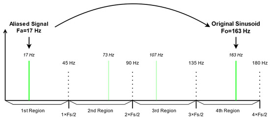
Figure 2.
Diagram showing the recovery of a signal from its aliased signal based on the Nyquist region where the signal belongs.
The frequency resolution (FR) is the gap between two neighbouring frequencies in the Fourier transform of a signal. This parameter determines the number of frequencies that can be used as identifiers within the range 0 to FN Hz. A smaller resolution allows for distinguishing more frequencies in the given range, but it also requires a longer signal ( seconds) to identify the frequency unequivocally. Longer capture times imply larger delays to detect a frequency and identify a light.
To be able to distinguish all frequencies from the selected set, they must be spaced apart by at least FR Hz. Hence, the frequency spectrum will be divided in bins. Note that the first bin, corresponding to , is discarded as it would not allow for distinguishing the frequency used from the constant component of a regular non-flickering light. Therefore, the frequency spectrum should be partitioned to accommodate the desired number of frequencies while excluding the constant range.
Figure 3 shows how many identifiers (number of frequencies) can be used depending on the duration of the signal and the camera frame rate. As an example, for an automated guided vehicle running at 2 m/s, a delay of 100 to 1000 ms to identify the lights would imply an initial period when the AGV would travel without positioning, from 20 to 200 cm.
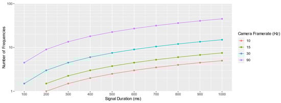
Figure 3.
Relation between the number of frequencies usable as identifiers and the duration of the captured signal for different camera frame rates.
The delay on the identification also limits the spacing of the lights, which must be visible for at least the required signal duration. Furthermore, to assure continuous positioning through all the area, the device must be able to identify new lights while at least four already identified lights are still visible and used for localisation purposes. This implies a minimal Field of View (FOV) of double for the distance travelled during the identification delay. Taking the 2 m/s AGV as an example, a FOV between 40 and 400 cm would be needed.
Equation (1) defines the coverage of a scenario, where FOVH and FOVV are the horizontal and vertical fields of view of the camera, GC and GR represent the columns and rows of the grid of lights and SR and SC refer to the spacing between rows and columns. As shown in Figure 3, with a signal duration of 1 s and a camera of 90 Hz, a maximum number of 45 identifiers can be used. From Equation (1), this case would only allow for covering an area of 120 m2 in a squared scenario (a 6 by 7 grid of lights taking into account that four references are necessary to solve the Perspective-n-Point problem).
To solve the coverage limitations of this identification method and make it scale to large scenarios, we have adopted a clustering approach. Concretely, the whole area is divided in clusters defined as a set of four neighbouring lights, each of them matching a unique pattern of frequencies. Using a simple 2D pattern-matching algorithm, a receiver would be able to link a cluster of frequencies with the pre-defined dataset of clusters. This would allow unique identification of the four components in the cluster.
Assigning the clusters of identifiers is not a trivial task, as each combination of four lights must be unique in the dataset, independent of the camera orientation. To avoid ambiguities, the clusters that could be confused based on their orientation are discarded and the rest are combined as efficiently as possible. Figure 4 illustrates the clustering approach for two different flickering frequencies and a 2 × 4 grid of lights. The colour of each light bulb indicates the flickering frequency, and the shape colour denotes the cluster of four lights that can be identified. As it can be observed, the central lights belong to two neighbouring clusters; thus, the whole grid is defined by four clusters, which can be unequivocally identified with only two frequencies.

Figure 4.
Example of the distribution of two frequencies into four clusters for a grid of 2 by 4 lights.
The clustering approach resolves the scalability issues for large scenarios. Concretely, for the previously mentioned scenario (90 Hz frame rate and 1 s signal duration), the size of the covered area increases from 120 to 82,880 m2 (8 ha), as calculated by Equations (2) and (3). However, the delay needed to identify lights cannot be entirely resolved, but it is mitigated. Ideally, to distinguish the required frequencies in the Fourier transform with the fewest samples, the signal duration should be adjusted to each scenario based on the positioning rate needs, the FOV of the camera and the speed of the moving vehicle.
Figure 5 shows two graphs that describe the relationship between the number of frequencies used in a scenario, the time needed to distinguish these frequencies and the number of potential clusters. It shows that the number of clusters grows exponentially with the size of the set of frequencies (number of frequencies), but the time needed to distinguish the frequencies of that set also grows and would influence the latency of the identification (and, thus, of the localisation). The number of potential clusters is described by the following equation:
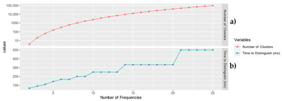
Figure 5.
(a) Evolution in the number of possible clusters for a set of frequencies. (b) Evolution in the minimum time to distinguish every frequency of a set.
As mentioned, each cluster consists of four lights. The equation presented in (3) can be used to determine the surface that a specific number of clusters can cover. This equation calculates how many overlapping squares exist in an N by M grid (being N ≥ M), and in this case, each square corresponds to a cluster.
For example, for 10 frequencies, Figure 5a shows that there would be 2599 clusters available. These clusters could be configured in a matrix of 24 by 26 lights, using 99.42% of the clusters available. For a separation of 1.2 m between lights, the light infrastructure would be able to span across a surface area of 497 m2. A combination between the Angle of Vision (AOV) of the camera and the height of the ceiling could achieve a FOV of 8 m, which would translate into coverage of 1182 m2 (Equation (1)). Figure 5b indicates that with 10 frequencies and a 90 Hz camera, the duration of the signal needed to distinguish the frequencies would be 250 ms, which corresponds to a frequency resolution of 4 Hz.
4. Hardware Components
The choice of the hardware components to implement our solution considered several factors. One of the main objectives was to demonstrate that the approach is feasible for low-budget equipment. Also, the dimensions of the receiver were considered, as it had to be placed in a mobile vehicle.
Figure 6 shows a simplified diagram of the solution, where we highlight the data flow. The light infrastructure implements an interface that allows its configuration via Wi-Fi. A microprocessor controls each light driver to switch at the corresponding flickering frequency. On the mobile device (receiver), the camera detects the flickering of visible light as a combination of (at least) four lights and finds their 2D to 3D coordinate correspondence in a pre-existent database. The coordinates of the identified lights are used to feed the positioning algorithm, returning the position of the mobile device (e.g., an AGV in a factory workspace).
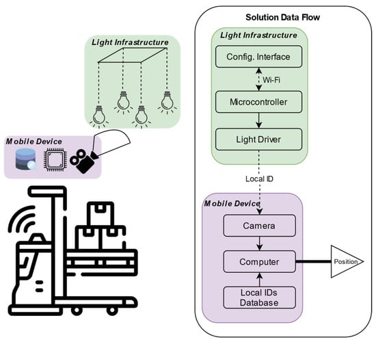
Figure 6.
Diagram of the proposed VLP solution.
4.1. Computing Unit
The computing unit must be an onboard device with enough computing capacity to run the software locally and in real time. Additionally, the solution should not depend on any specific hardware.
The equipment chosen to run our implementation is the Raspberry Pi 4B board [33] in the 8 GB RAM version, running the pre-installed Raspberry Pi 64-bit OS, which is based on a Debian Linux distribution. This low-cost computer integrates a quad-core ARM processor and Broadcom’s Videocore VI, which is a multimedia processor that allows displaying resolutions up to 4 K at 60 frames per second.
The popularity of both Raspberry Pi and its Linux-based operating system, together with the affordability of the hardware and a big developer’s community, makes it an attractive platform to demonstrate our solution.
4.2. Camera Unit
The size and cost of the camera must allow an easy and scalable deployment on a mobile asset. The camera unit must also be able to provide images at a high frame rate at a resolution of at least 720 p and should have a wide AOV. Most of the cameras that fulfil these size, cost and performance requirements are pinhole CMOS cameras that integrate a rolling shutter sensor.
Raspberry Pi offers the Camera Module 2 [34], which integrates Sony’s 8MP IMX290 CMOS image sensor [35]. This low-budget camera is one of the few that can run at a resolution of 1280 × 720 at 90 frames per second (FPS). When running at this speed, the camera cannot output the original resolution of 3280 × 2464 pixels and thus reduces the number of pixels by cropping the image, which therefore reduces the angle of vision down to 51 degrees for the horizontal axis and 30 degrees for the vertical axis. To overcome having a low FOV, a fisheye lens was added to the camera, achieving a final angle of vision of 82 and 42 degrees. Another method to expand the camera’s FOV is maximising the distance between the camera and the light infrastructure, although this aspect would highly depend on the conditions of the deployment scenario and the possibilities to install both the infrastructure and the mobile device in optimal locations.
Usually, camera sensor boards integrate their own feedback algorithms to adjust exposure, white balancing and gain to adapt to the changes in light of the scene. To simplify the evaluation of the repeatability of the software, all feedback algorithms were disabled, fixing all the parameters of the camera.
The shutter speed or exposition time is one of the most important parameters for our approach. It is common to see how cameras adjust this parameter to a multiple of the full period in the electrical network (depending on 50 or 60 Hz electrical network, 10 or 16 ms, respectively) to avoid the interference from lights that oscillate at this frequency. By setting the exposition time to be a multiple of the complete period, the luminosity of the network-synchronised light will always appear constant. However, in our case, as the oscillating frequencies are above 100 Hz, the exposition of the camera averages the luminosity of the lights across more than one state, effectively reducing the dynamic range of the signals. Therefore, the shutter speed of the camera was set to just one millisecond. At this speed, the camera could completely differentiate between the low and high state of the VLP lights, improving the dynamic range at the cost of perceiving the oscillation of the lights at the rate of the electrical network, needing a posterior filter.
Finally, the use of low-resolution images compromises the maximum achievable accuracy and even the maximum operational distance. While the characteristics of the Raspberry Pi fulfil our requirements for size and low budget, it is not capable to process the image frames of the camera at the maximum rate (90 FPS) and highest resolution. Therefore, we opted for the compromise of scaling down the original resolution of 1280 × 720 to 800 × 448.
4.3. Light Unit
For the light unit, the solution needs an LED illumination device with a microcontroller that can allow its wireless configuration and makes it possible to drive the light at the required frequencies.
The LEDs chosen are 10 watt A60 (60 mm wide) COTS light bulbs [36]. These bulbs incorporate an ESP 8266 [37] that controls the light’s temperature and intensity and also provides Wi-Fi connectivity for wireless control. The temperature can be adjusted from 3000 K to 6500 K. The light has a maximum luminosity of 810 lumens and a beam angle of 220°
These light bulbs integrate the Linkage’s SM2135E driver [38], which can be controlled via I2C with an Arduino library [39]. This driver allows for individually controlling the current of five channels: red, green, blue, warm white and cold white. With Arduino IDE’s [40] support for ESP devices, the microcontroller can be easily programmed, using the driver’s library, to modulate the light at a certain frequency, up to 5 kHz. The driver’s current-limiting capability allows for reducing the modulation depth by using two states of luminosity, instead of toggling between completely on and completely off states (OOK). This feature not only counteracts the loss in luminosity produced by the modulation itself, but also reduces the visibility of stroboscopic effects.
Additionally, the microcontroller can create a Wi-Fi interface to control and update the firmware wirelessly, using its over-the-air programming capabilities. However, although ESP’s popularity is rising, currently most light bulbs integrate different microcontroller–driver combinations that might not have such libraries and support.
In conclusion, at the time of the writing of this paper, the chosen hardware components can be classified as affordable as they cost less than 20 EUR per light bulb and less than 150 EUR for a complete VLP receiver device.
5. Positioning Software
The software we developed and installed in the computing unit takes advantage of its multiprocessing capabilities to process images at 90 FPS and produce positioning at the same rate. It is written in C++ and uses OpenMP (Version 4.5) [41] to enable the multiprocessing capabilities, and OpenCV to process the images, calculate the flickering frequency and estimate the position of the mobile device.
The software carries out the following tasks: (1) obtain image frames from the camera, (2) filter out interferences and identify potential lights, (3) track potential lights and record their characteristics, (4) calculate the frequency of the light’s dazzle, (5) match the spatial distribution of frequencies with a pre-loaded expected distribution, (6) solve the Perspective-n-Problem and (7) publish information through Wi-Fi. The code divides these tasks in three threads that run in parallel called Capturing, Processing and Publishing threads. Figure 7 contains a diagram of these threads and their tasks. This figure also depicts the data flow between threads and towards a common database named “LIGHT_LIST”, where no data races are possible due to multiple writings. Despite distributing the tasks among the cores, the pipeline of information makes the threads dependant on each other. Therefore, the tasks can only be executed concurrently, i.e., the capturing thread is obtaining and processing a new frame while the processing thread is working with the previous frame.
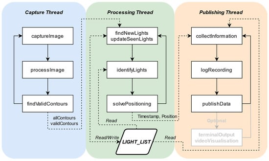
Figure 7.
Diagram of the software.
The Capturing thread performs task (1) and also task (2) to reduce load on the Processing thread. After receiving a new grey-scale frame from the camera, it performs a threshold-based binarisation. This threshold has been selected empirically to maximise the perceived variation on the signal emitted by the lights. Afterwards, the binarised image is further processed, using OpenCV’s contour detection algorithm, to find isolated regions. These contours are filtered based on their minimum and maximum size, their circularity coefficient and their proximity to other contours; discarding those contours whose size is too big or too small, those that do not have a round shape and those that are too close to each other. Finally, the area and coordinates of the centroid for each contour (potential light) are placed in a queue and handled to the Processing thread.
The Processing thread performs tasks (3), (4), (5) and (6). It stores the coordinates and area of potential lights (contours) and keeps track of them across consecutive frames. The dazzle (variation in the area) of a light serves as the signal for the Discrete Fourier Transform (DFT) to extract the flickering frequency. To distinguish between two nearby frequencies in the Fourier transform, the duration of the signal must be at least the inverse of the desired frequency resolution (FR). Therefore, after a light has been spotted for seconds, the process to find the flickering frequency starts.
After the DFT, a peak detection function returns the peaks of the Fourier transform that exceed by two times the standard deviation of the rest of the transform [42]. The resulting frequencies are converted to their original Nyquist region (Equation (4)) and are approximated to the nearest pre-defined frequency.
The approximation is achieved by calculating the absolute difference between the detected frequency and the frequencies of the set. The detected frequency is approximated to the set frequency whose difference is above the threshold, if any.
This threshold can theoretically be adjusted to the current FR of the signal (inverse of the duration), but empirical tests show that the minimal feasible frequency resolution would be 2 Hz with a 1 s signal duration. For additional robustness, the minimal frequency resolution was set at 3 Hz. Therefore, the threshold ranges from FR Hz to 3 Hz proportional to the number of samples of the signal, following Equation (5).
Equation (5) has the following variables:
- a is FR, which is the spacing between the frequencies used;
- b is 3, which is the empirical minimal frequency resolution with a 1 s signal;
- x is the current number of samples of the signal;
- xmin is the minimum number of samples, which is ;
- xmax is the maximum number of samples, which is 1 s times the frame rate.
To improve the robustness of the algorithm, we also implemented a weighted election process to determine the most probable flickering frequency in case of ambiguity.
Once a frequency has been elected, it is associated with the light. After the detection of at least four lights, the thread creates all the possible combinations of four, arranges them in a square formation and compares them to the pre-defined clusters. This procedure is called 2D pattern matching. If there is a match, the four matching lights receive a unique identifier that also enters a weighted election process. At this point, an unambiguously identified light can also determine its 3D coordinates in the real world.
The Perspective-n-Problem can be solved by providing a camera matrix, distortion coefficients and the correspondence between 2D image points and 3D object points. OpenCV’s solvePnP function provides multiple implementations to solve the problem. The implementation that has shown more coherent and consistent results was the ITERATIVE option.
The rotation and translation vectors (rvec and tvec) returned by solvePnP define the transformation of a 3D point to the camera coordinate frame. Inversely, to obtain the 3D coordinates of the camera in the frame of reference of the light infrastructure, the transformation detailed in Equation (6) is applied.
After obtaining the pose of the camera, this information is timestamped and queued. The Publishing process is used for debugging and development purposes. In this respect, it can log information, show a preview of the camera point of view, layout which contours are being used to position or interactively update some filtering parameters. However, all these features delay the processing. Thus, during the testing and evaluation phase, most features have been disabled, leaving only the task to store logs and to send the positioning information to the platform. The rate of the positioning messages sent to a remote platform can be configured depending on the real-time needs of the scenario. These messages include the last position estimated by the system and all the intermediate positions (historical data) calculated between two consecutive messages. This allows for reproducing the track followed by the mobile device in the remote platform even if the wireless link to transmit the information is limited.
In conclusion, we verified that in a normal operation the software is able to identify a new light and use it to position in less than 133 ms in 75% of the cases. From this time, about 100 ms are devoted to the minimum signal duration required to identify the frequencies and the remaining 33 ms can be attributed to a single identification mistake (frequencies are calculated every 3 frames, 33 ms). After this initial identification delay, the system can estimate a position at real time every 11 ms. To prevent incidents during this short initialisation phase (where no position can be computed, before identifying at least four valid lights), a mobile device (e.g., an AGV) could take actions to limit its speed or even stop until a valid position is calculated.
6. Infrastructure Validation
To validate the proposed IPS, we deployed two similar infrastructures in two different scenarios: our laboratory and a factory. While the laboratory infrastructure aided in testing, developing and evaluating the solution in a controlled scenario, the factory infrastructure presented a rougher environment that helped to identify flaws in the system and to improve the final robustness, demonstrating at the same time the applicability and feasibility of the solution.
6.1. Laboratory Testbed
This testbed was designed with the objective of becoming analogous to a real deployment in a factory. The infrastructure consisted of eight lights hung at 2.2 m from the floor in a four by two formation (Figure 8a), separated by 60 cm. The total dimensions of the infrastructure were 60 cm of width and 180 cm of length. On the floor of the laboratory (Figure 8b), we placed a measured grid with a granularity of 10 cm. The grid was used to map the positions of the lights in the floor and also to determine the precision of the system to locate fixed and mobile items.
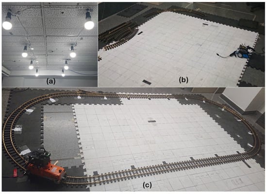
Figure 8.
Laboratory testbed. (a) The VLP lights hanging from the ceiling in a 4 by 2 formation. (b) The measured grid on the floor, each line is separated 10 cm. (c) The train tracks above the grid with pass-through identifiable marks.
To analyse the impact of the stroboscopic effect in our system, we conducted a test where the SVM was calculated using the toolbox described in [43]. We tested four of our lights (the minimum set to estimate a position), placing the sensor on the floor at the centre of the lights. The test was performed in complete darkness and the SVM was estimated to be 0.35. When turning on the other lights in the laboratory (fluorescent lights), the SVM fell to 0.13. These results indicate that the minimal light infrastructure needed to provide positioning produces a non-visible stroboscopic effect that complies with the current European normative [31].
An HO-scale train was used to test the performance of the system with mobility because it assures a fixed trajectory and can travel at different speeds. At maximum speed, the train travelled at an average of 78 cm/s. Tests were also performed at a lower speed (in average, 12 cm/s) to validate the impact of the speed on the accuracy of our system.
Placing the tracks above the grid (Figure 8c) allowed for measuring the position of the track junctions and reproducing the ground-truth path. Additionally, a camera was fixed to the ceiling to verify at which instant the train crossed each track junction. This setup allows synchronisation between the positions calculated by the device and the location of the train at every moment, to measure the 2D precision of the solution and to estimate the latency of the solution.
6.2. Factory Testbed
We collaborated with Bosch Aranjuez in the context of the European project IoT-NGIN [44] to deploy a VLP infrastructure in an actual factory environment, where robots are used to carry items. In [45], the authors present some preliminary results of this deployment together with other technologies (CV, UWB and AR) focusing on preventing collisions and incidents in a factory environment.
The deployed VLP infrastructure, as depicted in Figure 9b, consisted of eight lights in a four by two formation with a spacing of 1.2 m. This structure was suspended at a height of 4.2 m from the floor. In total, the light structure spanned 1.2 m in width and 3.6 m in length.

Figure 9.
Pictures of the factory testbed. (a) Factory’s AGV with the installed VLP receiver device. (b) Infrastructure of installed lights. (c) Detailed view of the VLP device in the front of the AGV.
In this deployment, it was not possible to place a measured grid on the floor; thus, measurements could not be taken across the surface like in the laboratory testbed. Instead, the camera had to be placed under each light, whose position was already precisely surveyed, to calculate the precision of the system.
To evaluate the robustness, performance and precision of the solution in this environment, we taped a circuit onto the floor that travelled in a straight line through all the lights in a zigzag pattern. The VLP device was attached to a small line-follower robot that provided repeatability to the tests. The aim of the line-follower robot was to provide complementary experiments for different mobility patterns, a feature that was not possible with the factory AGV. The straight line segments allowed for estimating the precision in movement.
Finally, we installed the receiver hardware on an AGV (Figure 9a,c) that travels under the lights to collect positioning results in an actual operative environment. The placement of the hardware on the AGV had to balance the resulting field of view with the visual obstructions produced by the robot’s body. Placing the camera at the lowest possible surface increases the FOV and therefore the distance at which the camera starts viewing the lights of the ceiling; however, the robot itself blocks part of this gained field of view, obstructing some of the lights prematurely. Figure 10 shows the point of view of the camera at the lowest possible placement on the AGV. On the left side, the sequence of images shows how the upper structure of the robot obstructs the lights prematurely.
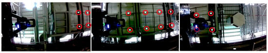
Figure 10.
Sequence of images from the point of view of the VLP device while travelling beneath the infrastructure. The red circles indicate the lights of the infrastructure. The dashed circle shows the position of a light that is not visible due to the obstruction of the AGV.
7. Data Analysis
For every test in the laboratory scenario, we store additional information related to the calculated position, such as the identifier of the lights used for the estimation. With this additional information, it was possible to perform a post-analysis and evaluate multiple conditions or scenarios beyond the one in which the test was conducted. During the post-processing, every positioning achieved with more than four lights can be recalculated using a reduced number of lights. This allows for evaluating scenarios with fewer lights, analysing the impact of light spacing, and identifying possible mispositioned lights. The groups of lights, or clusters, are depicted in the diagram shown in Figure 11, and are defined as follows:

Figure 11.
Diagram showing the nomenclature for the data analysis.
- A, B and C define the original clusters of four lights, where all the lights are separated 60 cm apart. Cluster B shares two lights with cluster A and the other two with cluster C.
- D1 and D2 also use only four lights, but the separation between them is 60 cm in one direction and 120 cm in the other. Specifically, D1 is defined by lights b01, b02, b05 and b06; D2 is defined by lights b03, b04, b07 and b08.
- Cluster E uses the edge lights (b01, b02, b07, b08). These lights are separated 60 cm in one direction and 180 cm in the other.
- Cluster AB and BC use six lights, combining the lights of two clusters.
- Cluster ABC uses eight lights, all the available lights.
Additionally, the clusters can be grouped into low-density or high-density scenarios. The results obtained by using only four lights (clusters A, B, C, D1, D2 and E) would be a low-density scenario and those using more than four lights (clusters AB, BC and ABC) correspond to a high-density scenario. From the point of view of deployment costs, a configuration where the number of lights per square metre is minimal is the most favourable one. However, there might be a compromise between the infrastructure’s density of lights and the achievable precision.
8. Results
This section presents the results from all the tests conducted. We evaluated the precision of the solution in fixed positions and with mobility. These evaluations were conducted in the laboratory and factory environments. Finally, we evaluated the dynamic precision of the device when attached to the AGV in operative conditions.
8.1. Laboratory Static Tests Results
These tests were conducted in the laboratory testbed, placing the VLP device directly on the floor. The measured grid of the laboratory allowed for measuring positioning errors in twenty spots at four different orientations. In our coordinate system, the light infrastructure formed a rectangle from [−60, 0] to [120, 60] cm, approximately. The positions tested were located as follows:
- Ten positions were at the borders of the infrastructure;
- Eight positions were outside the borders of the infrastructure, separated 60 cm in the Y-axis;
- Two positions were inside the borders of the infrastructure.
Figure 12 shows an overall image of all the tests performed across the surface of the laboratory, the opacity of the points and segments is used to visualise the distribution in the precision. The red rectangle represents the light infrastructure, which does not appear completely regular because the lights were manually fixed to the ceiling. As noted previously, there is no specific geometric requirement for the Perspective-n-Point to be solved.
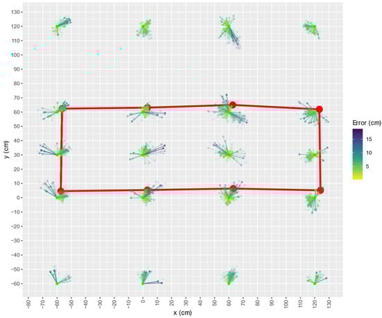
Figure 12.
Scatterplot showing the points obtained in the static tests. The green dots denote the real positions of the device. The calculated positions are connected to the real position with a line coloured by the distance to this point. The red rectangle indicates the structure of the lights.
The results obtained show that the number of lights per square metre (density) has no significant impact on the precision of the solution. As Figure 13 depicts, accuracy improves when more than four lights are used for positioning or when the spacing between lights is larger. This could indicate that increasing the separation between lights is beneficial for both coverage and accuracy.
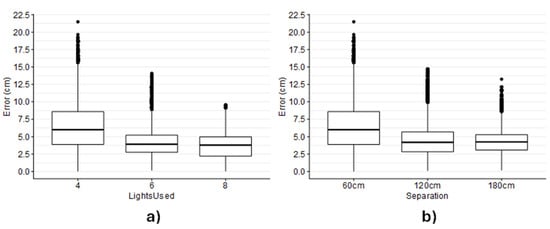
Figure 13.
Boxplots showing (a) the error by the number of lights used to position and (b) the separation between the lights (only in one of the axes) when only four lights are used to position.
8.2. Laboratory Dynamic Tests Results
These tests were carried out at the laboratory testbed, attaching the VLP device to the train with the camera installed at the centre of the train and its widest side oriented perpendicular to the direction of travel.
In this setup, no individual four-light cluster was visible from every point in the track. For this reason, we could not evaluate the precision in a low-density scenario.
Before performing dynamic tests using the train, some static measurements were performed at the junctions between train tracks to establish a baseline for the dynamic error.
8.2.1. Track Junctions Static Test Results
The train was placed on each track junction, where a static test was conducted. Figure 14 shows that there is a common absolute error on the top region of the graph, from y = 90 upwards. This error is approximately 10 cm and is directed inwards.

Figure 14.
Scatterplot showing the distribution in the error on the track’s junctions. The green dots determine the real position. The calculated positions are connected to the real position with a line coloured by the distance to this point. The red square indicates the structure of lights. The black line indicates the centre of the train track.
The LOESS (Locally Estimated Scatterplot Smoothing) curve in Figure 15 indicates that the error could be symmetrical in the axis depending on the location relative to the infrastructure of lights. A reason for this behaviour might be an inaccurate identification of the centre of the light bulbs when the camera has a distant and sided perspective.
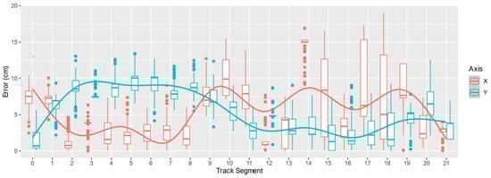
Figure 15.
Boxplot showing the error in the X and Y axis for each track junction.
8.2.2. Train Mobility Test Results
In the mobility tests, a camera fixed at the ceiling of the laboratory was used to verify the real position of the train. This camera recorded at 90 FPS at a resolution of 640 by 480 pixels. The camera was synchronised with the positioning camera on the train via Network Time Protocol (NTP) synchronisation and annotated the timestamp in every frame.
A total of three tests were conducted for each speed. The duration of the high speed (78 cm/s) tests was 60 s, and the duration of the low speed (12 cm/s) tests was 180 s. The recordings were examined manually, and we noted the timestamp at which the train’s camera passed through each of the track junction marks. We selected the first position reported by the camera’s positioning software after these timestamps.
As with the static tests, there is a clear deviation inwards of the error for points above y = 90. Additionally, Figure 16a,b show all the points computed by the positioning program. It denotes some displacement of approximately 5 cm at the transitions where the number of lights used for positioning changes.
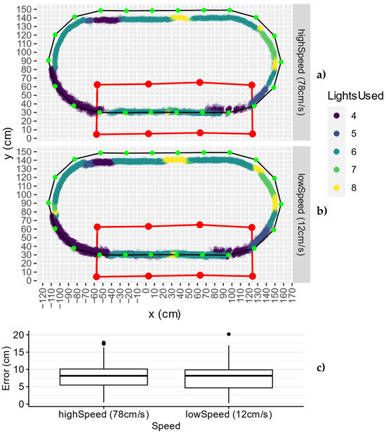
Figure 16.
Scatterplot showing the positions calculated at (a) high speed and (b) low speed. The red rectangle represents the infrastructure of lights. The black line represents the centre of the train track. The green dots are the real positions at the train track junctions. The colour of the points represents the number of lights used to calculate that position. (c) Boxplots of the errors measured in these tests by different speeds.
Figure 16c shows how the overall error is practically equal between the two speeds and that it is less than 10 cm in 75% of the occasions. This indicates that speed is most likely not detrimental to the accuracy in an actual factory deployment, where speeds of 120 cm/s could be reached.
8.3. Factory Static Test Results
In the factory deployment, static measurements were only performed in the points under each of the eight lights.
Figure 17a shows an overall image of all the static tests. The maximum error is found at the top-right corner. As observed in the laboratory scenario, Figure 17b,c show that accuracy improves with the number of lights used and the separation between them. However, despite the separation of lights is larger in the factory than in the laboratory, the results are not better. This could be explained by the difference in height, which increased from 2.2 m in the laboratory to 4.2 m in the factory.
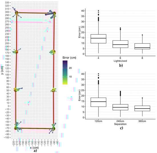
Figure 17.
(a) Scatterplot showing all of the points obtained in the static tests in the factory. The green dots define the real position. The calculated positions are connected to the real position with a line coloured by the distance to this point. Boxplots showing the error in static positioning in the factory depending on (b) the number of lights used to position and (c) the separation between the lights for 4-light positioning.
8.4. Factory Mobility Test Results
To evaluate the performance of our solution in a factory environment, we decided to conduct two tests. The first one evaluated the accuracy and performance of the solution and the second one provided a baseline that could be compared with the AGV tests.
8.4.1. Multiple Orientation Tests
To test the precision and performance with mobility, we depicted a path in the floor formed by straight lines between each light projection (see Figure 18). These tests demonstrated the capability of the system to position a device at any point inside the covered area, and its reliability and robustness, as the robot would view the scenario in different orientations, which increases the chances of receiving interference from other light sources.
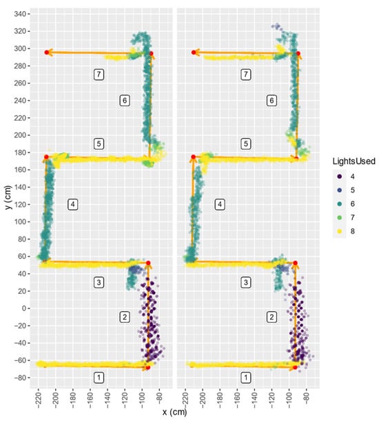
Figure 18.
Scatterplot showing the positions calculated with the line follower test. The orange arrows indicate the lines and the direction of the movement. The colours represent how many lights were used to calculate that position. The labels indicate the segment number.
Figure 18 shows the scatterplot for the tests. For reference, we name each straight line as “segment” starting with number 1 at the bottom and ending with 7 at the top. In general, both tests look very similar, which demonstrates repeatability. Though the first test shows fewer points for segment 7, this discrepancy is not related to the positioning algorithm, but to an early finalisation of the data collection service.
The 16:9 aspect ratio of the camera sensor implies a FOV that depends on the orientation of the camera; therefore, although being in the centre of the testbed (segment 4), the camera is unable to see all eight lights. Figure 19 shows the boxplots of the error in the zigzag tests with the line follower coloured by the orientation of the robot. The reason why the horizontal orientation (segments 1, 3, 5 and 7) achieves better results is because the wide side of the sensor is parallel to the testbed, and therefore is able to see all the lights. Additionally, the second segment shows a significantly higher error variation, which is explained by a slight tilt between the camera and the robot that limits the number of lights (only four) viewed from that location.
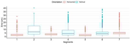
Figure 19.
Boxplot showing the error in the zigzag test with the line follower in the factory for each segment and orientation.
8.4.2. Straight Line Tests
For these tests, with the objective of simulating the trajectory of a real AGV using the line follower robot, we placed tape in a straight line on the centre of the road that spanned 8 m long.
Figure 20a shows the results for one of the tests where the line follower robot moved in a straight line. The robot was travelling from bottom to top, which explains that, as it approaches the infrastructure of lights, firstly it views only four lights, then six and finally all eight lights. The coverage of the lighting infrastructure is greater than the depicted line, but we limited the test, from Y = −350 to Y = 400, to match the area covered by the AGV tests in an operative environment. Figure 20a also depicts a regression line to evaluate how much the line follower diverted from the ground truth. The angle difference is only 1° (note that the proportions shown in the figure exaggerate the deviation). The position of the lights was verified to assure that the deviation was not caused by an imprecision in the measurement of the reference coordinates. Thus, it was concluded that this deviation must be caused by another source that is more difficult to correct, such as the difference in height between the lights or the inclination of the camera.
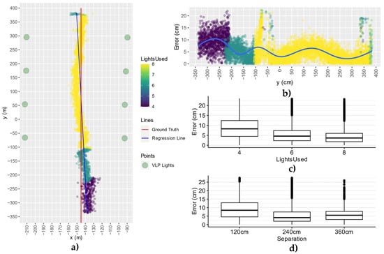
Figure 20.
(a) Scatterplot showing one trajectory with the line follower robot following a straight line. The VLP camera was oriented with the widest side parallel to the infrastructure. (b) Scatterplot showing the error in the X-axis for all the tests. Boxplots showing the error (c) depending on the number of lights used and (d) depending on the separation of the lights.
The error between the points calculated in the tests and the ground truth was measured. The results are shown in Figure 19c and Figure 20b,d. Figure 20b depicts the error analysed for every point of the Y axis, in the direction of the movement. For the points directly under the testbed (eight lights case), the error is below 6.5 cm for 75% of the measured samples. As it can be seen in Figure 20c, the error is significantly higher for four lights.
Note that the accuracy of the tests is similar to the one achieved in the horizontal segments (with eight lights) for the multiple orientation scenario.
Compared to the static tests, interestingly, the mobile scenario outperforms them in terms of accuracy, as the results show an average improvement of 5.5 cm. This indicates that a device running through the middle of the light infrastructure may achieve a more accurate position than a device on the sides of the infrastructure. This fact is relevant for deciding how to deploy the VLP infrastructure.
8.5. Real Factory Deployment
After the mobile and static tests, a VLP device was attached to an AGV, as depicted earlier in Section 6.2. (Figure 9a), that passes several times under the VLP’s light infrastructure during its common operation. Currently, we have collected data for 138 trajectories of the AGV out from 16 days of recording.
Figure 21 shows three representative examples of these trajectories captured in different days during a span of a week, to avoid any correlations based on the day of the recording. The colour of the points in the plot indicates how many lights were used to calculate the positioning. For reference, the AGV travelled in the direction bottom to top. Therefore, as the robot entered the covered region, the positioning was calculated first with four, then with six and finally with eight lights. Unfortunately, due to the visual obstruction of the lights caused by the AGV’s own structure, the time the AGV spends positioning with eight lights (and therefore, with the maximum accuracy) is reduced. This behaviour is visualised in Figure 10, as the point of view of the camera shows how the back part of the AGV blocks the light on the left side of the image. Additionally, Figure 21 denotes that the AGV can be positioned 270 cm (Y = −340) before entering the light infrastructure, but only 20 cm (Y = 340) after leaving the area beneath the light infrastructure. This is explained by a forward tilt of the camera, manually adjusted to minimise the obstruction of the AGV without compromising the accuracy.
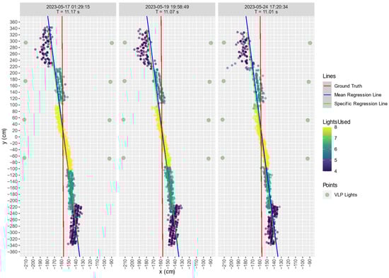
Figure 21.
Annotated scatterplot for three trajectories where the VLP device was placed on the AGV.
Additionally, Figure 21 shows three different coloured lines. The red line is denoted as ground truth and corresponds to the estimated path that the AGV is following. This path was built from measurements of a real trajectory, where the AGV was forced to stop at several points. The blue line, labelled as the mean regression line, represents the regression line obtained from all the points of all the trajectories tracked for the AGV. The green line, tightly overlapping with the blue line, is the regression line calculated only with the points of each specific trajectory.
Figure 22a shows the scatterplot for the error against the ground truth for 62 trajectories where the AGV had travelled under the infrastructure without stopping. As can be observed, the best results were achieved under eight lights and the worst at the transitory sections (using only four and six lights), especially when the robot was leaving the infrastructure (right side).
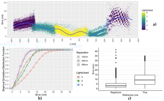
Figure 22.
(a) Scatterplot showing the error in 62 non-stopping trajectories of the AGV compared to the ground truth. (b) Empirical cumulative distribution function of the error using a different number of lights and for different light separations. (c) Boxplot showing the residuals for the AGV dataset calculated for the regression line and the ground truth.
Figure 22c shows the boxplots for the error in the same 62 trajectories. The boxplot showing the error against the mean regression line proves repeatability on the positioning of the trajectory of the AGV. The boxplot showing the error against the ground truth indicates that the positioning error in the AGV is generally less than 15 cm.
Figure 22b contains the empirical cumulative distribution functions of the error when analysing the impact of the number of lights used for the positioning and the separation between them. It shows that the best accuracy, under 10 cm in 90% of the occasions, is achieved using eight lights separated by 120 cm and also with four lights and a separation of 360 cm. Additionally, the transitory sections where not all eight lights can be seen (at the start and end of the covered area) provide an acceptable accuracy below 12 and 20 cm, for six and four lights, respectively, in 90% of the occasions.
For the AGV tests, the deviation between the average positioning trajectory and the ground truth is 3.2°, which is 2.4° more than what we would expect based on the line follower results. However, considering that the error is not correlated to the length of the testbed, this deviation falls within the expectations for the current scenario. For instance, in a worst-case scenario, error might shift by −20 cm at the beginning of the testbed and by +20 cm at the end, resulting in a 3.27° deviation angle for the current length. Nevertheless, if the error remains constant, the deviation will rectify itself for longer distances.
9. Discussion
In this work, we developed and evaluated a low-budget system designed to accurately position a moving vehicle within a factory environment. Our approach tackles the Perspective-n-Point problem by employing a novel method of identification to establish 2D–3D correspondence that, through undersampling, avoids relying on the rolling shutter effect, the size of the LED light or the distance from it.
To enhance the scalability of this new identification method, we introduced a spatial constraint, where the combinations of four locally identified lights (due to the four-point requirement to solve the Perspective-n-Point problem) were used to identify them globally. This spatial constraint took the form of a rectangle of lights in our case, but this geometry could be adapted to the existing lighting configuration in a factory.
We showed that a Raspberry Pi 4 computer connected to a pinhole camera operating at 90 FPS was able to calculate positioning at the same rate as the image influx of the camera. This feat was achieved by running custom optimised software that uses computer vision techniques to filter interferences and identify the lights. The positioning time achieved by our solution, 11 ms, is significantly faster that other similar solutions such as those reported in [17,18], which achieved 44 ms (Raspberry Pi 3) and 162 ms (Intel i5-6600), respectively.
The possibility of performing some or all the operations using edge or cloud computing can also be considered as it can offer much higher processing capability. This extra capacity can be used for higher resolution images or even running multiple positioning algorithms in real time. However, ensuring wireless communication in real time with a roundtrip time below eleven ms would pose disadvantages: firstly, it would add complexity to the solution, which implies adding points of failure; secondly, having a stable and fast internet connection at all times would depend on deploying additional Wi-Fi access points or using 5G, if available; and thirdly, the wireless communication is susceptible to radio frequency interferences, which would eliminate VLP’s advantage in environments prone to interference. Moreover, the embedded device would require a non-negligible computing power to be able to capture and to compress high-resolution images for the edge or cloud computer to process them. In other words, edge or cloud computing would not be advantageous over the locally processing solution implemented because it would impair the scalability, increase the cost and increase the complexity of the solution.
The possibility of performing some or all the operations using edge or cloud computing can also be considered as it can offer much higher processing capability. This extra capacity can be used for faster image acquisition cameras or better resolution images. However, this solution implies sending images wireless. This must be done by keeping the delay in image processing (compressing locally, transferring to the processing facility, uncompressing, processing, obtaining location and sending back this information for navigation) under the order of ms. For example, with the present settings the total roundtrip time must be under 11 ms. To this difficulty we must add the continuous wireless connectivity and the fact that the bandwidth available should be shared among the different robots moving in the premises. Connectivity can be provided, for example, by Wi-Fi or private 5G, but considering the complexity of industrial environments, this bandwidth might result difficult to achieve. In other words, edge or cloud computing probably would not reduce the cost and complexity of the locally implemented processing solution.
The achieved positioning rate of 90 Hz almost reaches the recommended positioning rate of 100 Hz for outdoor automated vehicles, making it suitable for indoor AGVs. It could also be complemented with IMUs for dead-reckoning to meet the 100 Hz positioning rate recommendation.
The novel method of identification offers flexibility, as it could use existing lighting by just installing a modulator, albeit with reduced illumination efficiency. Alternatively, additional lighting containing specific firmware could be installed. For this project, we deployed an infrastructure comprising eight COTS light bulbs running a simple firmware that flickered the light without producing visible stroboscopic effects, adhering to European recommendations [31].
The deployed infrastructure is complementary to the current lighting infrastructure of the factory, to avoid disturbing the operational environment, but also to test the coexistence of the solution with existing lightning systems, and even with visible light communication devices such as Li-Fi. The added lights are low power devices in comparison to the light used in these environments, easy to install (they only require a connection to AC), affordable (they are consumer-grade) and incorporate the light driver and the communication capabilities for its remote configuration.
The positioning system has been initially tested in a laboratory with a controlled environment and finally validated in actual deployment. This deployment had a limited extension, only eight lights. This size is perfect for analysing the effect of specific situations, such as the delay in the first identification or the loss of reference lights (e.g., temporary occlusions). At the same time, the deployment is large enough to estimate the performance of the system in a large-scale deployment, where the loss of reference lights would be infrequent.
The infrastructure, spanning 1.2 m wide and 3.6 m long, installed in an actual factory at a height of 4.2 m, delivered accurate positioning despite the presence of interference coming from other sources of light. It achieved a maximum coverage of 9.5 m on the longest axis and a typical coverage of 7 m during AGV tests (with partial FOV obstruction). From the operational AGV tests, we can conclude that we were able to consistently position from a distance in the range between 4.2 and 5.7 m, whereas the authors in [10,12] presented similar results only in the range between 0 and 3 m.
The interferences produced by the specific lighting infrastructure in the factory (skylights, fluorescents and LED) were discarded using filtering techniques based on size, shape and distribution. However, the parameters related to each of the filters are specified for each environment and would require an initial verification for each deployment. For better performance, it is recommended that the lights used at the location are similar and uniformly distributed.
We tested the accuracy and performance of the system by conducting static and mobility tests in the laboratory testbed. In 75% of the cases, static tests achieved accuracy below 6 cm, while mobility tests remained below 10 cm.
The static test results revealed that accuracy is significantly influenced by the number of lights used for positioning and the separation between the lights when employing only four of them. These factors also appeared significant in the static tests in the factory environment. However, other factors such as the vertical distance to the lights, which increased from 2.2 to 4.2 m, hampered the accuracy and explain why despite having up to six-fold separation between lights, results were worse than in the laboratory (below 14 cm in 75% of the occasions). Additionally, the camera’s location within the testbed was a minor factor affecting accuracy. Placing the VLP device at the edges or outside the infrastructure led to errors of up to 10 cm compared to positioning it directly beneath the infrastructure.
In the laboratory mobility tests, we found that the positioning accuracy of the tracked vehicle was affected neither by movement (compared to static tests) nor by different moving speeds.
Furthermore, we attached our VLP device to an AGV that operated in the factory on a daily basis and recorded dozens of trajectories in various lighting conditions (sunlight plus artificial lighting during day, artificial lighting only during night). We analysed 62 non-stopping trajectories and measured an accuracy below 7.2 cm in 75% of the occasions and below 12 cm in 95% of the occasions when eight lights were used for positioning.
We demonstrated that the same accuracy can be achieved by using only four lights separated by 360 cm in one axis. Therefore, for future and larger deployments, it would be advisable to maximise the separation between the lights to increase the solution coverage and to reduce the required infrastructure.
10. Conclusions
Indoor positioning systems have been applied to multiple scenarios, and they are crucial for the navigation of automated guided vehicles in the industry, where these vehicles present opportunities to improve the scalability and efficiency of industrial processes. A precise and reliable positioning system is crucial, not only to automate these processes, but also to ensure a safe coexistence between automated vehicles and humans, especially in environments where loud noises, distractions and radio interference could lead to dangerous interactions between automated vehicles and humans.
Automated guided vehicles usually depend on two complementary positioning systems: one for navigation across the factory and another for precise operations such as difficult manoeuvres or cargo loading. Most of the current indoor positioning systems struggle when balancing the coverage and the accuracy of the solution, and VLP is no different. However, we propose a solution that embraces the features of a VLP system to provide a two-in-one solution for navigation and precise operation, while also enhances its current coverage and scalability capabilities.
VLP stands out over other infrastructureless IPS (such as SLAM) because it requires no learning of the environment and is resilient to changes that would invalidate other systems (such as modifications on the operational layout) as long as the lighting infrastructure remains in place.
Most IS-VLP solutions rely on the combination of the rolling shutter effect and light coding schemes to identify a VLP light, which is the crucial step before calculating positioning. This method of identification has multiple flaws, such as the limited positioning distance (depending on the shape and size of the VLP lights and the camera resolution) and a scalability problem, which hampers the appeal of this technology over others to provide positioning in a factory environment.
Our work represents a significant step towards enhancing the competitiveness of VLP compared to other positioning technologies. The proposed system can reuse existing LED-based lighting (at the cost of replacing the light driver) independently of its shape, size or height. The solution is fully scalable and can fit diverse needs, from covering a small area where precise location would be needed to cover the entire factory. The proposed system is not limited to pre-defined moving paths; it can locate in 3D objects anywhere within the covered area. The positioning rate is aligned with the recommendations for moving vehicles in a factory environment. The design is robust to the presence of other sources of light not involved in the location, light reflections and sunlight coming from skylights.
A real autonomous guidance is achieved within the device that is embedded to a moving object, implemented with low-cost hardware in terms of image sensors (cameras) and processors, which demonstrates the cost-effectiveness of the solution.
In this work, we developed an indoor positioning system that achieves an accuracy of 7.2 cm when positioning an autonomous guided vehicle travelling at speeds up to 1.20 m per second, providing position updates at a rate of 90 positions per second within an actual factory environment.
Even though we covered all the identified requirements such as scalability, affordability, accuracy and reliability, we also identified the benefits of further improving the performance, facilitating the deployment and adding new functionalities.
The positioning error could be reduced by using better image sensors with improved resolutions and faster image processing, while keeping the same algorithms. Also, a higher image acquisition rate would allow for tracking faster-moving AGVs. Certainly, these improvements should be accompanied by more powerful computing to cope with these image processing requirements. Nevertheless, improving hardware capabilities is not an uncommon practice in industrial applications.
For less demanding deployments, methods to further increase the coverage without losing on accuracy could be explored, such as the optimal location or inclination of the VLP receiver on the moving vehicle to prevent occlusion, or the use of wider fisheye lenses.
Finally, as the study has focused on navigation, only 2D accuracy has been tested, despite calculating six-axis positioning, including pose and height. For asset location purposes, for example, in warehouses, the performance in the third dimension could also be considered, which could be combined with the pose to determine the direction of travel, and, for example, a more precise estimation of the alert zone volume.
Author Contributions
Conceptualisation, J.P. and M.C.; methodology, A.B.; software, A.B. and C.L.; validation, A.B. and C.L.; formal analysis, A.B.; investigation, A.B., C.L., J.P. and M.C.; data curation, A.B.; writing—original draft preparation, A.B.; writing—review and editing, J.P., M.C. and C.L.; visualisation, A.B.; supervision, J.P. All authors have read and agreed to the published version of the manuscript.
Funding
This research received funding from the Departament de Recerca de Universitats de la Generalitat de Catalunya under grant 2021 SGR 01524, from the European Union’s Horizon 2020 research and innovation programme under Grant Agreement No. 957246 (project IoT-NGIN) and from the Spanish MCIN/AEI/10.13039/501100011033 through project PID2019-106808RAI00.
Institutional Review Board Statement
Not applicable.
Informed Consent Statement
Not applicable.
Data Availability Statement
Data are contained within the article.
Acknowledgments
The authors acknowledge the technical and logistic support provided by Bosch Aranjuez staff during the deployment of the factory tests.
Conflicts of Interest
The authors declare no conflicts of interest.
References
- Trevlakis, S.E.; Boulogeorgos, A.-A.A.; Pliatsios, D.; Querol, J.; Ntontin, K.; Sarigiannidis, P.; Chatzinotas, S.; Di Renzo, M. Localization as a Key Enabler of 6G Wireless Systems: A Comprehensive Survey and an Outlook. IEEE Open J. Commun. Soc. 2023, 4, 2733–2801. [Google Scholar] [CrossRef]
- Mendoza-Silva, G.M.; Torres-Sospedra, J.; Huerta, J. A Meta-Review of Indoor Positioning Systems. Sensors 2019, 19, 4507. [Google Scholar] [CrossRef] [PubMed]
- Reid, T.G.R.; Houts, S.E.; Cammarata, R.; Mills, G.; Agarwal, S.; Vora, A.; Pandey, G. Localization Requirements for Autonomous Vehicles. arXiv 2019, arXiv:1906.01061. [Google Scholar] [CrossRef]
- Adame, T.; Igual, J.; Catalan, M. Fast Deployment of a UWB-Based IPS for Emergency Response Operations. Sensors 2023, 23, 4193. [Google Scholar] [CrossRef] [PubMed]
- Jang, B.; Kim, H.; Kim, J. Wook Survey of Landmark-Based Indoor Positioning Technologies. Inf. Fusion 2023, 89, 166–188. [Google Scholar] [CrossRef]
- Huang, J.; Junginger, S.; Liu, H.; Thurow, K. Indoor Positioning Systems of Mobile Robots: A Review. Robotics 2023, 12, 47. [Google Scholar] [CrossRef]
- European Commission Directive 2011/65/EU of the European Parliament and of the Council of 8 June 2011 on the Restriction of the Use of Certain Hazardous Substances in Electrical and Electronic Equipment (Recast) (Text with EEA Relevance). Off. J. Eur. Union OJ L 174 2011, 54, 88–110. Available online: http://data.europa.eu/eli/dir/2011/65/oj (accessed on 14 December 2023).
- Maheepala, M.; Kouzani, A.Z.; Joordens, M.A. Light-Based Indoor Positioning Systems: A Review. IEEE Sens. J. 2020, 20, 3971–3995. [Google Scholar] [CrossRef]
- Danakis, C.; Afgani, M.; Povey, G.; Underwood, I.; Haas, H. Using a CMOS Camera Sensor for Visible Light Communication. In Proceedings of the 2012 IEEE Globecom Workshops, Anaheim, CA, USA, 3–7 December 2012; IEEE: Piscataway, NJ, USA, 2012; pp. 1244–1248. [Google Scholar] [CrossRef]
- Liang, Q.; Lin, J.; Liu, M. Towards Robust Visible Light Positioning Under LED Shortage by Visual-Inertial Fusion. In Proceedings of the 2019 International Conference on Indoor Positioning and Indoor Navigation (IPIN), Pisa, Italy, 30 September–3 October 2019; IEEE: Piscataway, NJ, USA, 2019; pp. 1–8. [Google Scholar] [CrossRef]
- Kuo, Y.S.; Pannuto, P.; Hsiao, K.J.; Dutta, P. Luxapose: Indoor Positioning with Mobile Phones and Visible Light. In Proceedings of the 20th Annual International Conference on Mobile Computing and Networking, Maui, HI, USA, 7–11 September 2014; pp. 447–458. [Google Scholar] [CrossRef]
- Rahman, M.H.; Sejan, M.A.S.; Chung, W.Y. Multilateration Approach for Wide Range Visible Light Indoor Positioning System Using Mobile CMOS Image Sensor. Appl. Sci. 2021, 11, 7308. [Google Scholar] [CrossRef]
- Li, Z.; Chen, G.; Wang, A. Indoor Positioning System Using Visible Light Communication and Smartphone with Rolling Shutter Camera. Ph.D. Dissertation, UC Riverside, Riverside, CA, USA, 2016. [Google Scholar]
- Hong, C.H.; Nguyen, T.; Le, N.T.; Jang, Y.M. Modulation and Coding Scheme (MCS) for Indoor Image Sensor Communication System. Wirel. Pers. Commun. 2017, 93, 987–1003. [Google Scholar] [CrossRef]
- Ferrandiz-Lahuerta, J.; Camps-Mur, D.; Paradells-Aspas, J. A Reliable Asynchronous Protocol for VLC Communications Based on the Rolling Shutter Effect. In Proceedings of the 2015 IEEE Global Communications Conference (GLOBECOM), San Diego, CA, USA, 6–10 December 2015; IEEE: Piscataway, NJ, USA, 2015; pp. 1–6. [Google Scholar] [CrossRef]
- OpenCV Documentation. Version 4.5.5. Available online: https://docs.opencv.org/4.5.5/ (accessed on 14 December 2023).
- Lin, P.; Hu, X.; Ruan, Y.; Li, H.; Fang, J.; Zhong, Y.; Zheng, H.; Fang, J.; Jiang, Z.L.; Chen, Z. Real-Time Visible Light Positioning Supporting Fast Moving Speed. Opt. Express 2020, 28, 14503. [Google Scholar] [CrossRef] [PubMed]
- Guan, W.; Chen, X.; Huang, M.; Liu, Z.; Wu, Y.; Chen, Y. High-Speed Robust Dynamic Positioning and Tracking Method Based on Visual Visible Light Communication Using Optical Flow Detection and Bayesian Forecast. IEEE Photonics J. 2018, 10, 1–22. [Google Scholar] [CrossRef]
- Hussain, B.; Wang, Y.; Chen, R.; Yue, C.P. Camera Pose Estimation Using a VLC-Modulated Single Rectangular LED for Indoor Positioning. IEEE Trans. Instrum. Meas. 2022, 71, 1–11. [Google Scholar] [CrossRef]
- Cao, M.W.; Jia, W.; Zhao, Y.; Li, S.J.; Liu, X.P. Fast and Robust Absolute Camera Pose Estimation with Known Focal Length. Neural Comput. Appl. 2018, 29, 1383–1398. [Google Scholar] [CrossRef]
- Vakhitov, A.; Colomina, L.F.; Agudo, A.; Moreno-Noguer, F. Uncertainty-Aware Camera Pose Estimation from Points and Lines. In Proceedings of the 2021 IEEE/CVF Conference on Computer Vision and Pattern Recognition (CVPR), Nashville, TN, USA, 21–25 June 2021; IEEE: Piscataway, NJ, USA, 2021; pp. 4657–4666. [Google Scholar] [CrossRef]
- Mehralian, M.A.; Soryani, M. EKFPnP: Extended Kalman Filter for Camera Pose Estimation in a Sequence of Images. IET Image Process. 2020, 14, 3774–3780. [Google Scholar] [CrossRef]
- Lee, T.E.; Tremblay, J.; To, T.; Cheng, J.; Mosier, T.; Kroemer, O.; Fox, D.; Birchfield, S. Camera-to-Robot Pose Estimation from a Single Image. In Proceedings of the 2020 IEEE International Conference on Robotics and Automation (ICRA), Paris, France, 31 May–31 August 2020; pp. 9426–9432. [Google Scholar] [CrossRef]
- Rego, M.; Fonseca, P.; Alves, L.N. Transmitter Position Error Impact on Camera Based Visible Light Positioning Systems. In Proceedings of the 2022 4th West Asian Symposium on Optical and Millimeter-wave Wireless Communications (WASOWC), Tabriz, Iran, 12–13 May 2022; IEEE: Piscataway, NJ, USA, 2022; pp. 1–6. [Google Scholar] [CrossRef]
- Amsters, R.; Demeester, E.; Slaets, P.; Holm, D.; Joly, J.; Stevens, N. Towards Automated Calibration of Visible Light Positioning Systems. In Proceedings of the 2019 International Conference on Indoor Positioning and Indoor Navigation, IPIN 2019, Pisa, Italy, 30 September–3 October 2019; Institute of Electrical and Electronics Engineers Inc.: Piscataway, NJ, USA, 2019. [Google Scholar] [CrossRef]
- Lin, Y.T.; Yang, Y.H.; Fang, S.H. A Case Study of Indoor Positioning in an Unmodified Factory Environment. In Proceedings of the 2014 International Conference on Indoor Positioning and Indoor Navigation (IPIN), Busan, Republic of Korea, 27–30 October 2014; pp. 721–722. [Google Scholar] [CrossRef]
- Barbieri, L.; Brambilla, M.; Pitic, R.; Trabattoni, A.; Mervic, S.; Nicoli, M. UWB Real-Time Location Systems for Smart Factory: Augmentation Methods and Experiments. In Proceedings of the 2020 IEEE 31st Annual International Symposium on Personal, Indoor and Mobile Radio Communications, London, UK, 31 August–3 September 2020. [Google Scholar] [CrossRef]
- Pudu Robotics PuduBot2: Smart Delivery Robot. Available online: https://www.pudurobotics.com/product/detail/pudubot2 (accessed on 12 December 2023).
- Perz, M.; Vogels, I.; Sekulovski, D.; Wang, L.; Tu, Y.; Heynderickx, I. Modeling the Visibility of the Stroboscopic Effect Occurring in Temporally Modulated Light Systems. Light. Res. Technol. 2015, 47, 281–300. [Google Scholar] [CrossRef]
- Bullough, J.; Hickcox, K.S.; Klein, T.; Lok, A.; Narendran, N. Detection and Acceptability of Stroboscopic Effects from Flicker. Light. Res. Technol. 2012, 44, 477–483. [Google Scholar] [CrossRef]
- Commission Regulation (EU) 2019/2020 of 1 October 2019 Laying down Ecodesign Requirements for Light Sources and Separate Control Gears Pursuant to Directive 2009/125/EC of the European Parliament and of the Council and Repealing Commission Regulations (EC) No 244/2009, (EC) No 245/2009 and (EU) No 1194/2012 Text with EEA Relevance. Off. J. Eur. Union OJ L 315 2019, 209–240. Available online: http://data.europa.eu/eli/reg/2019/2020/oj (accessed on 14 December 2023).
- Perz, M. Opinion: Setting the Stroboscopic Visibility Threshold. Light. Res. Technol. 2020, 52, 322. [Google Scholar] [CrossRef]
- Raspberry Pi 4 Model B Specifications. Available online: https://www.raspberrypi.com/products/raspberry-pi-4-model-b/specifications/ (accessed on 14 December 2023).
- Raspberry Pi Camera Module 2 Specifications. Available online: https://www.raspberrypi.com/products/camera-module-v2/ (accessed on 14 December 2023).
- SONY IMX219 CMOS Image Sensor Datasheet. Available online: https://www.opensourceinstruments.com/Electronics/Data/IMX219PQ.pdf (accessed on 14 December 2023).
- Electro DH LED LightBulb 81.209/WIFI/A60. Available online: https://www.electrodh.com/catalogo/ver-item.action?id=33153&d=1 (accessed on 14 December 2023).
- ESP8266 Wi-Fi MCU Datasheet. Available online: https://www.espressif.com/sites/default/files/documentation/0a-esp8266ex_datasheet_en.pdf (accessed on 14 December 2023).
- SM2135E Five-Channel Intelligent Dimming LED High-Voltage Linear Constant Current Driver IC (Chinese). Available online: https://www.sohu.com/a/685179435_121491473 (accessed on 3 October 2023).
- jonodav SM2135-Arduino: Arduino Library for Interfacing with SM2135 LED Drivers. Version 20 July 2020. Available online: https://github.com/jonodav/SM2135-Arduino (accessed on 3 October 2023).
- Arduino IDE 2. Available online: https://docs.arduino.cc/software/ide-v2 (accessed on 29 May 2023).
- OpenMP Application Programming Interface. Version 4.5. Available online: https://www.openmp.org/wp-content/uploads/openmp-4.5.pdf (accessed on 14 December 2023).
- Brakel, J.P.G. van Robust Peak Detection Algorithm Using Z-Scores. Version 8 November 2020. Available online: https://stackoverflow.com/questions/22583391/peak-signal-detection-in-realtime-timeseries-data/22640362#22640362 (accessed on 14 December 2023).
- Banerjee, K. Stroboscopic Effect Visibility Measure Toolbox. Version 1.2.0.0. Available online: https://www.mathworks.com/matlabcentral/fileexchange/59242-stroboscopic-effect-visibility-measure-toolbox (accessed on 6 September 2023).
- IoT-NGIN. Available online: https://iot-ngin.eu/ (accessed on 25 October 2023).
- Catalan, M.; Hjeij, M.; Boixader, A.; Bonett, P.; Montagud, M.; Escrig, J.; Brugues, J.; Adame, T.; Labella, C.; Huerta, I.; et al. Towards IoT Ambient Intelligence for Industry 4.0. In Proceedings of the 2023 International Conference of Internet of Things and Cloud (FiCloud), Marrakesh, Morocco, 14–16 August 2023. [Google Scholar]
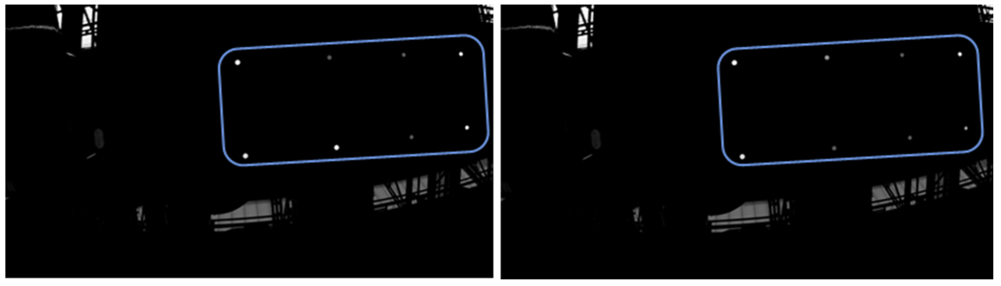
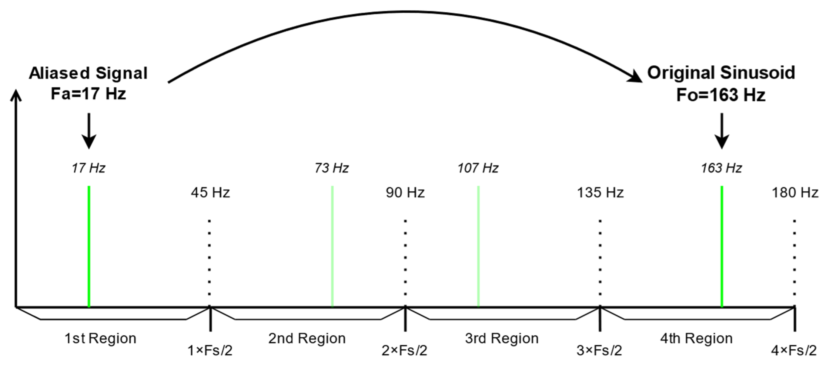
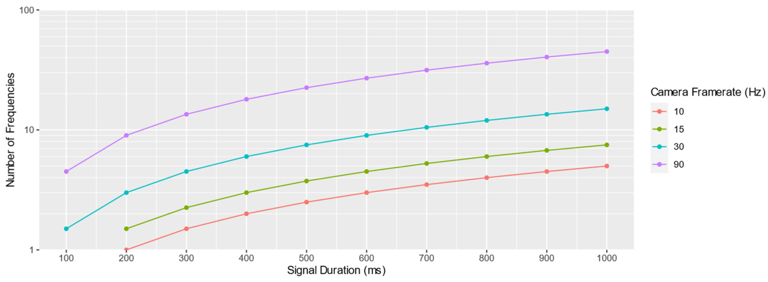
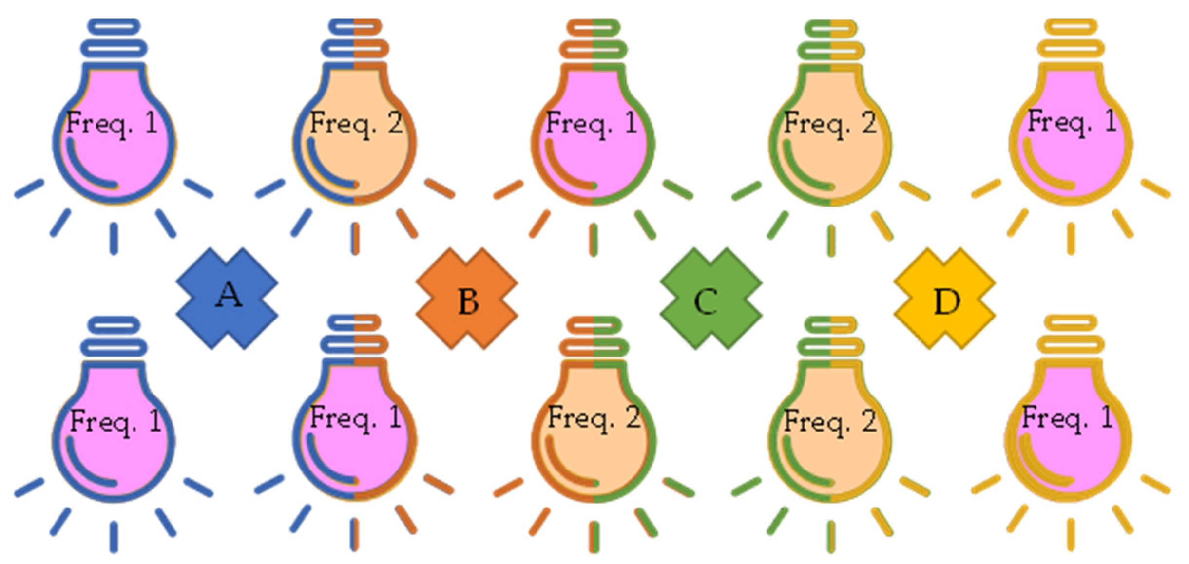
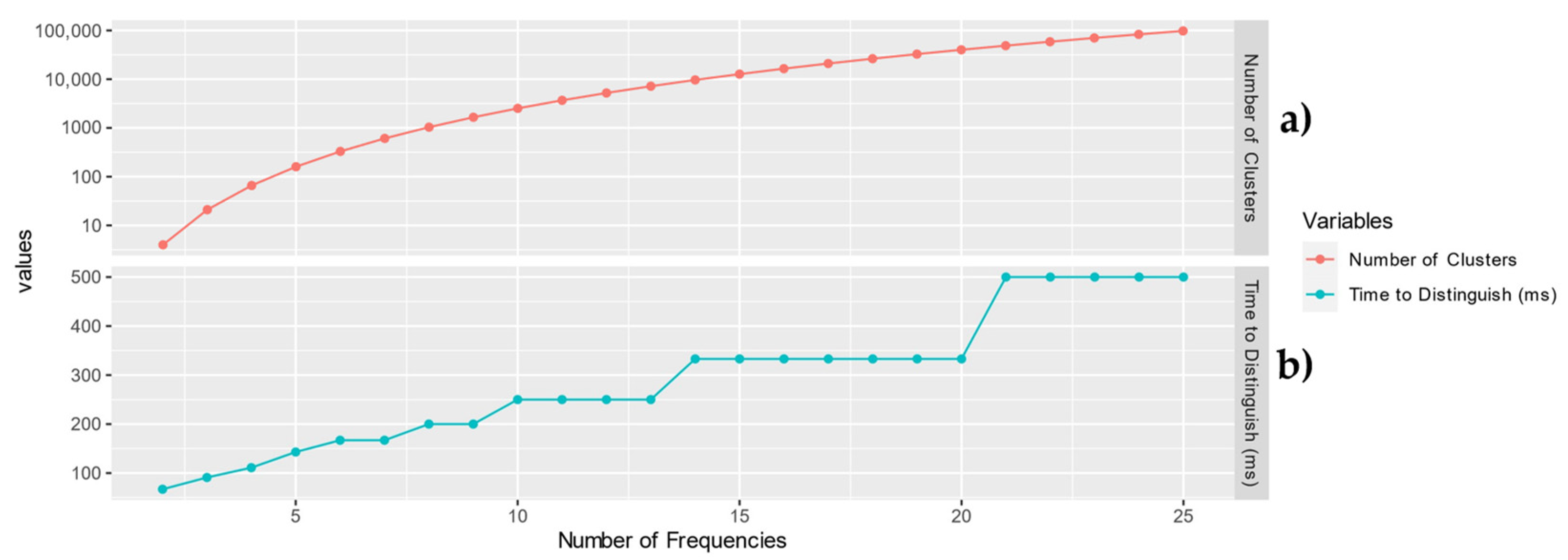

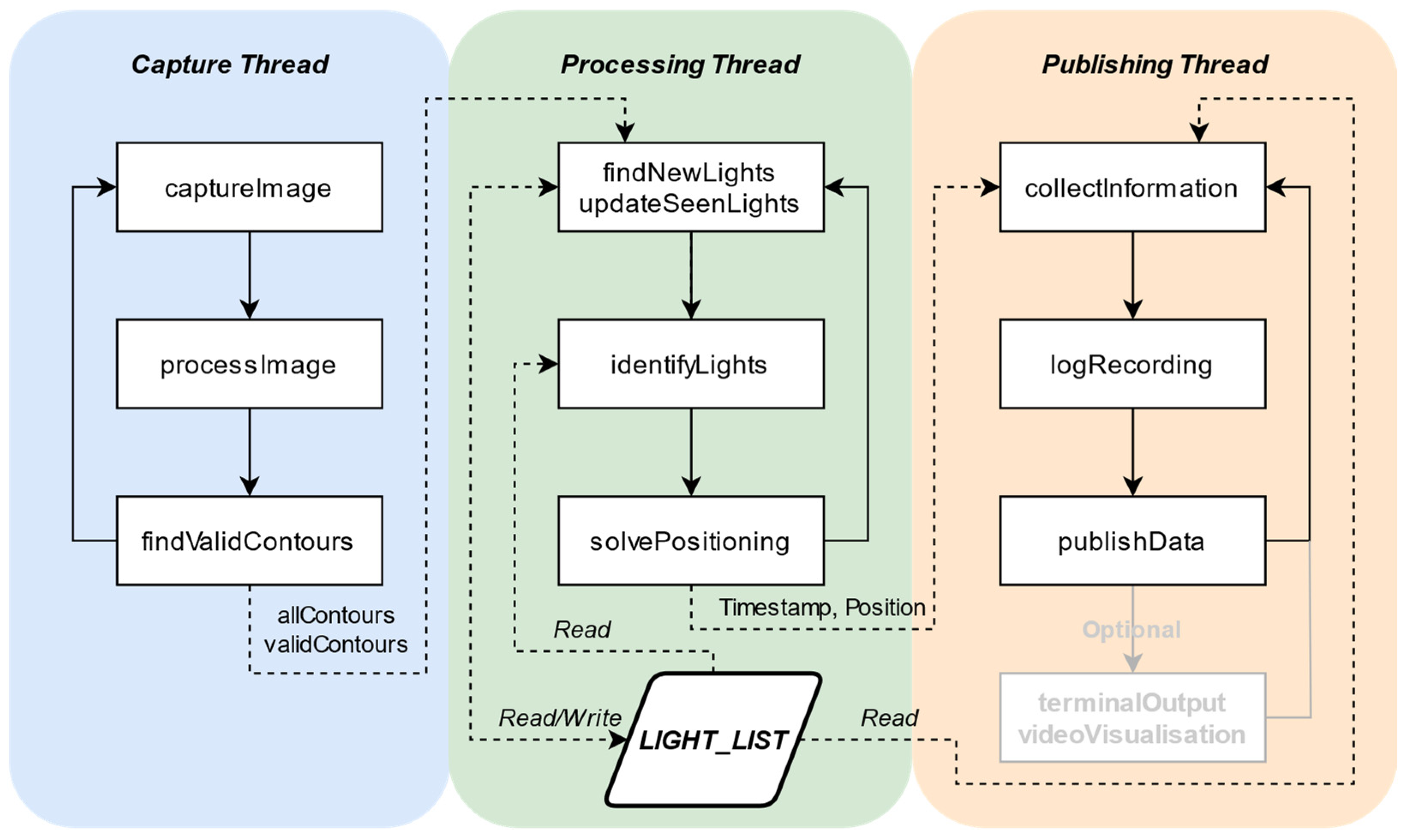
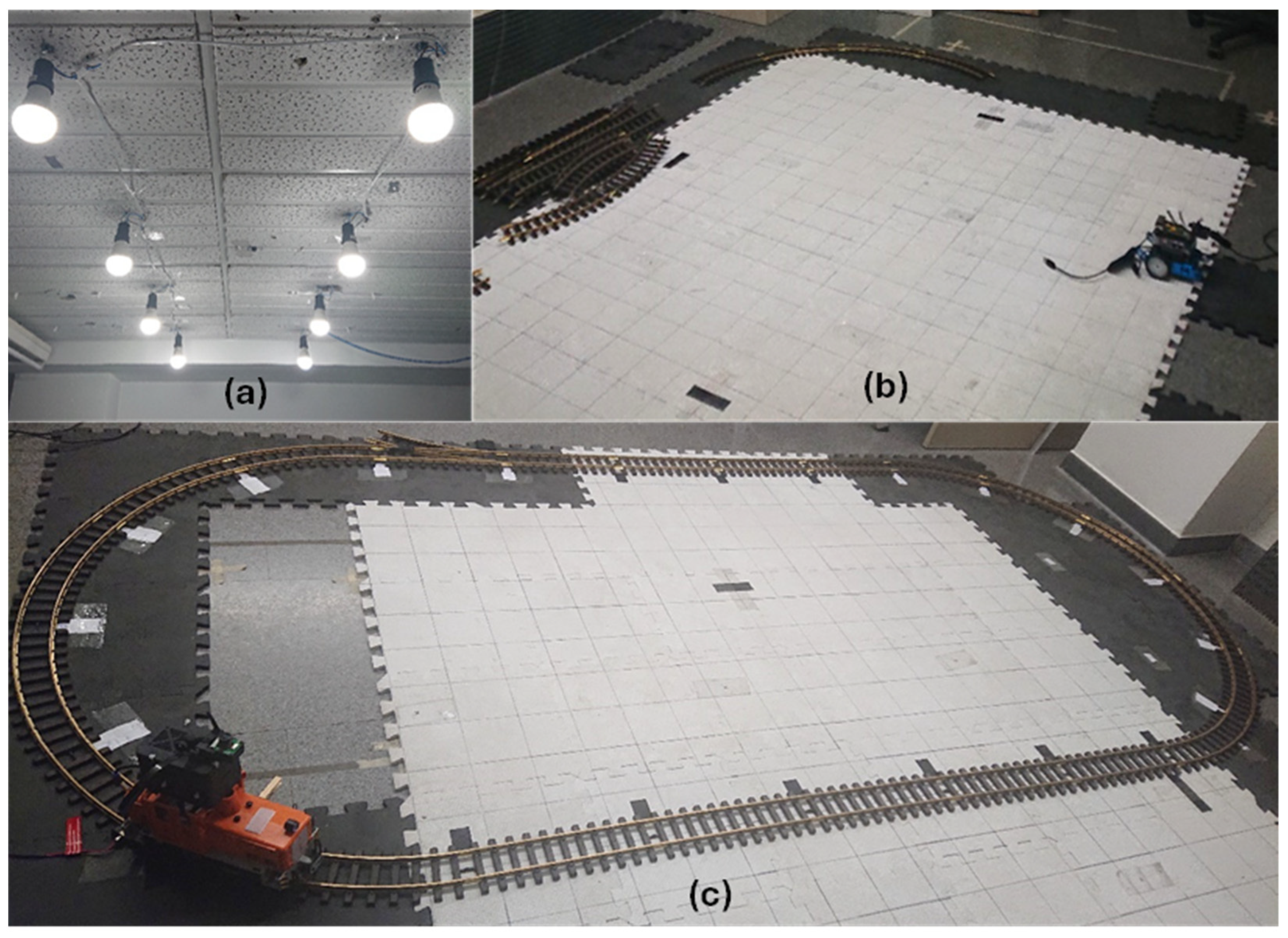
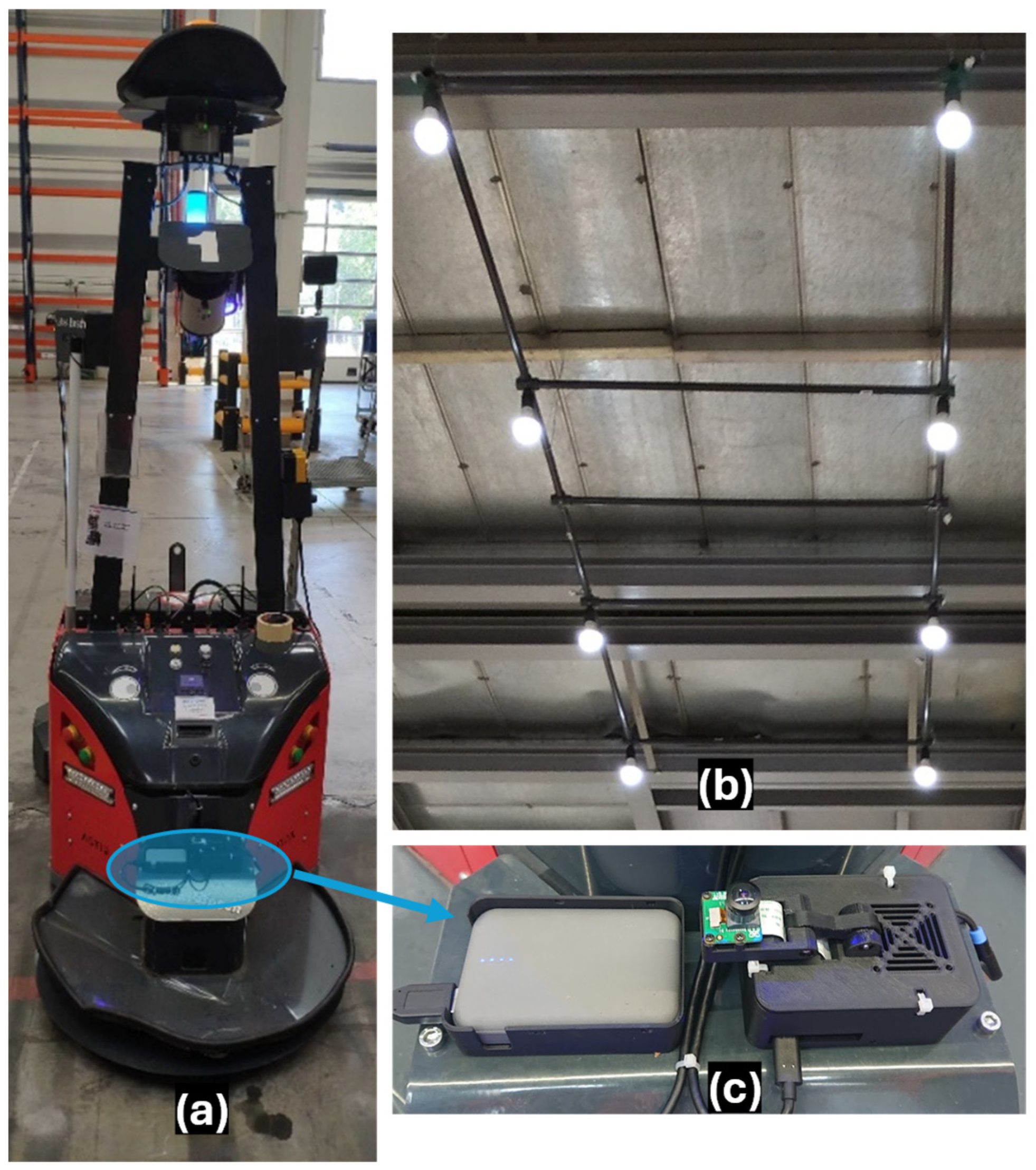
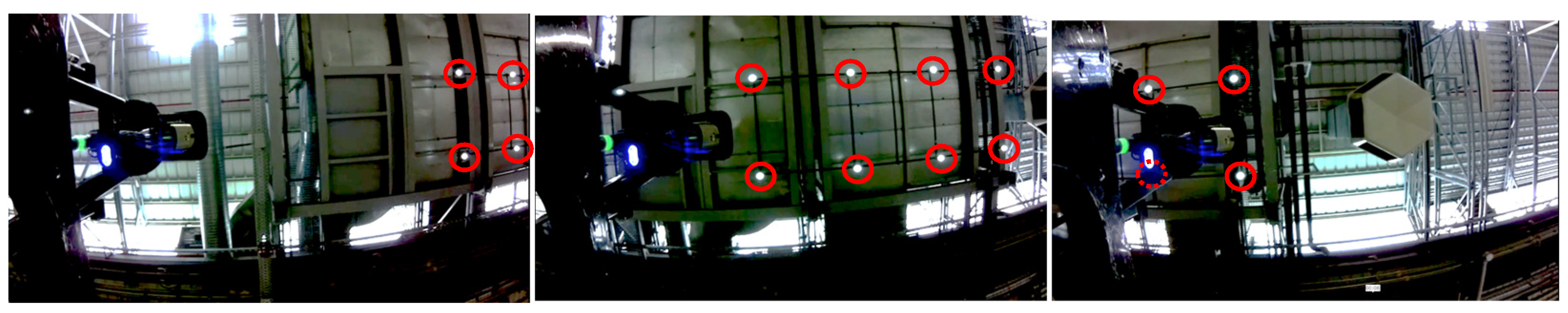
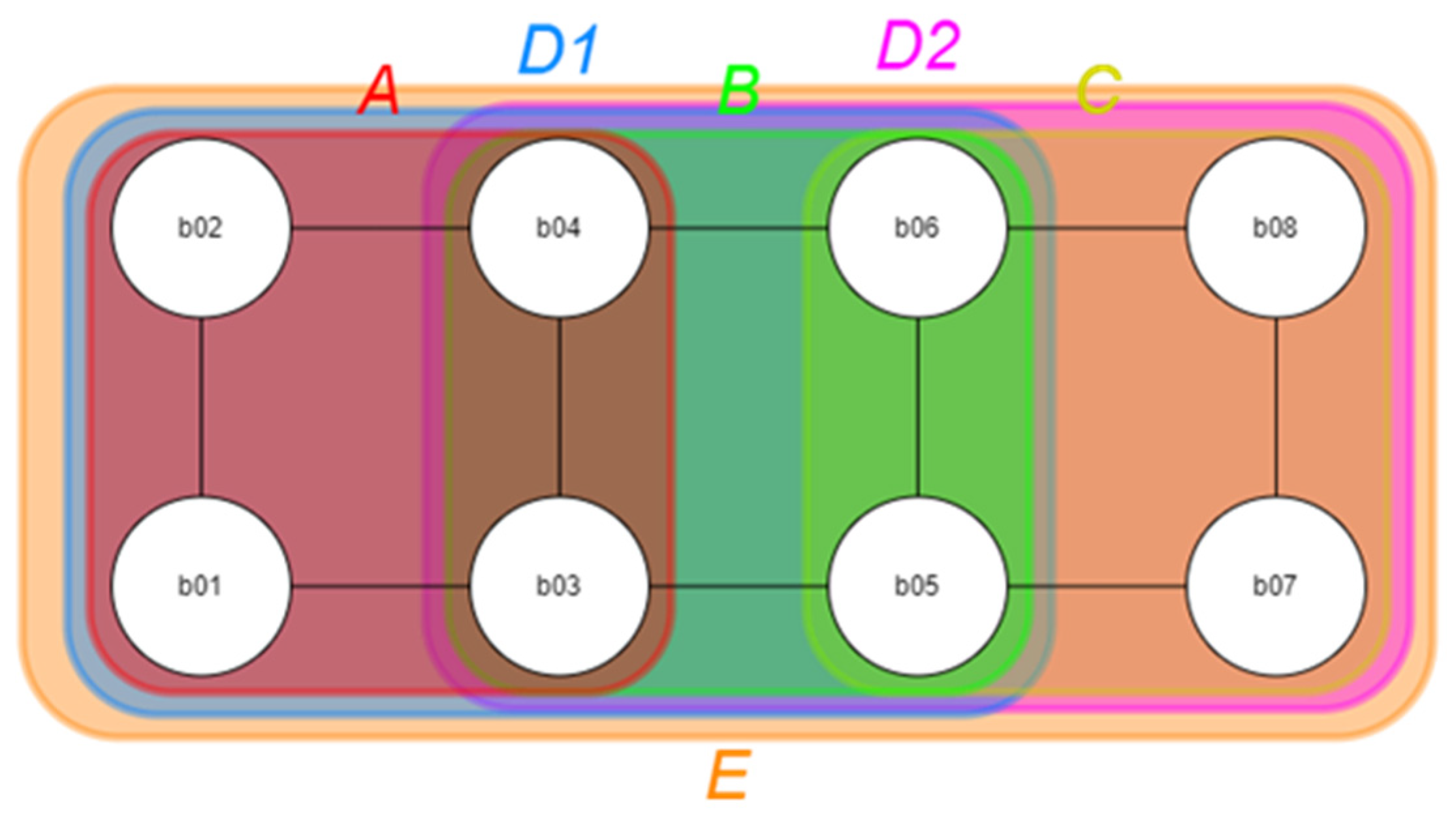
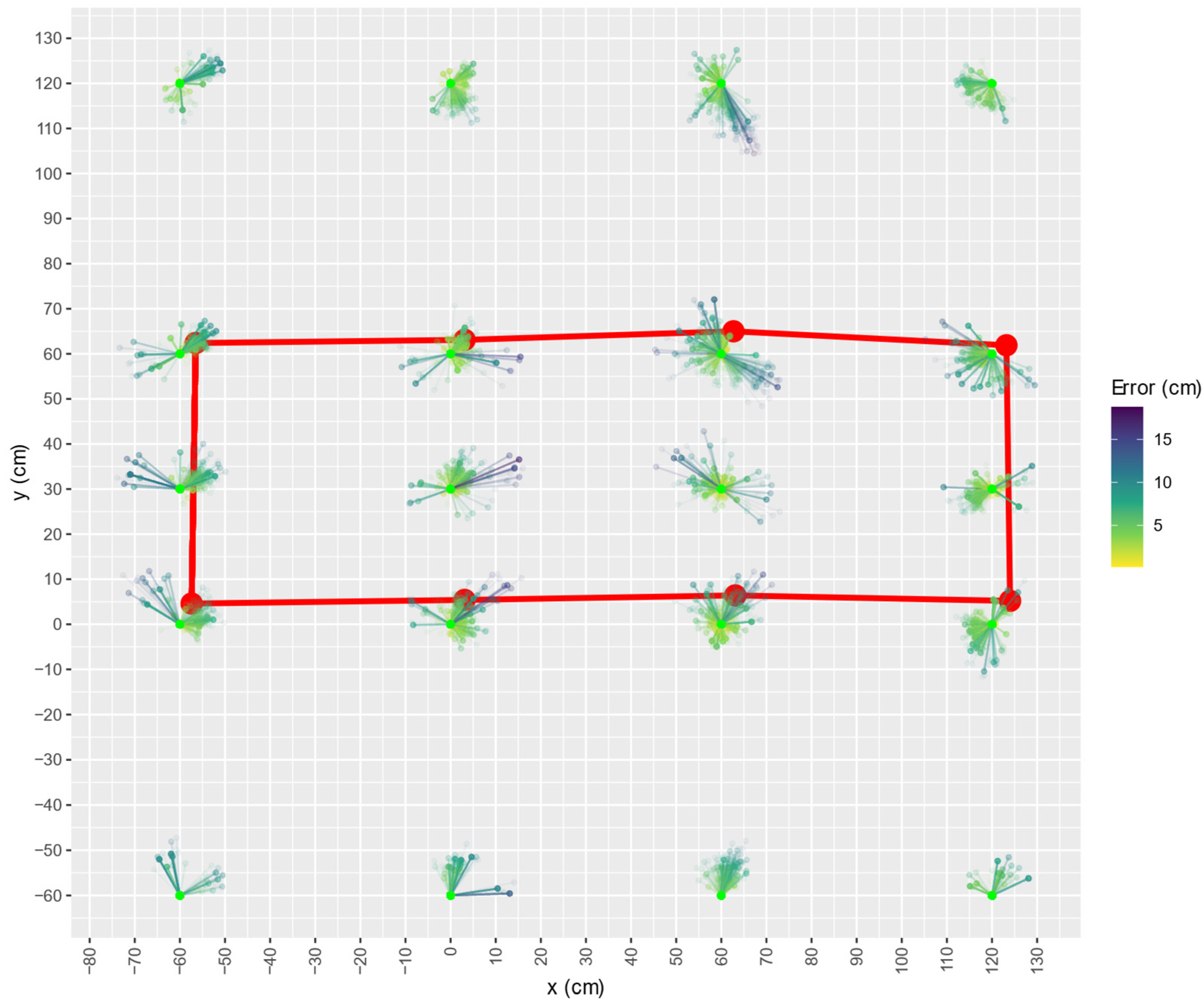
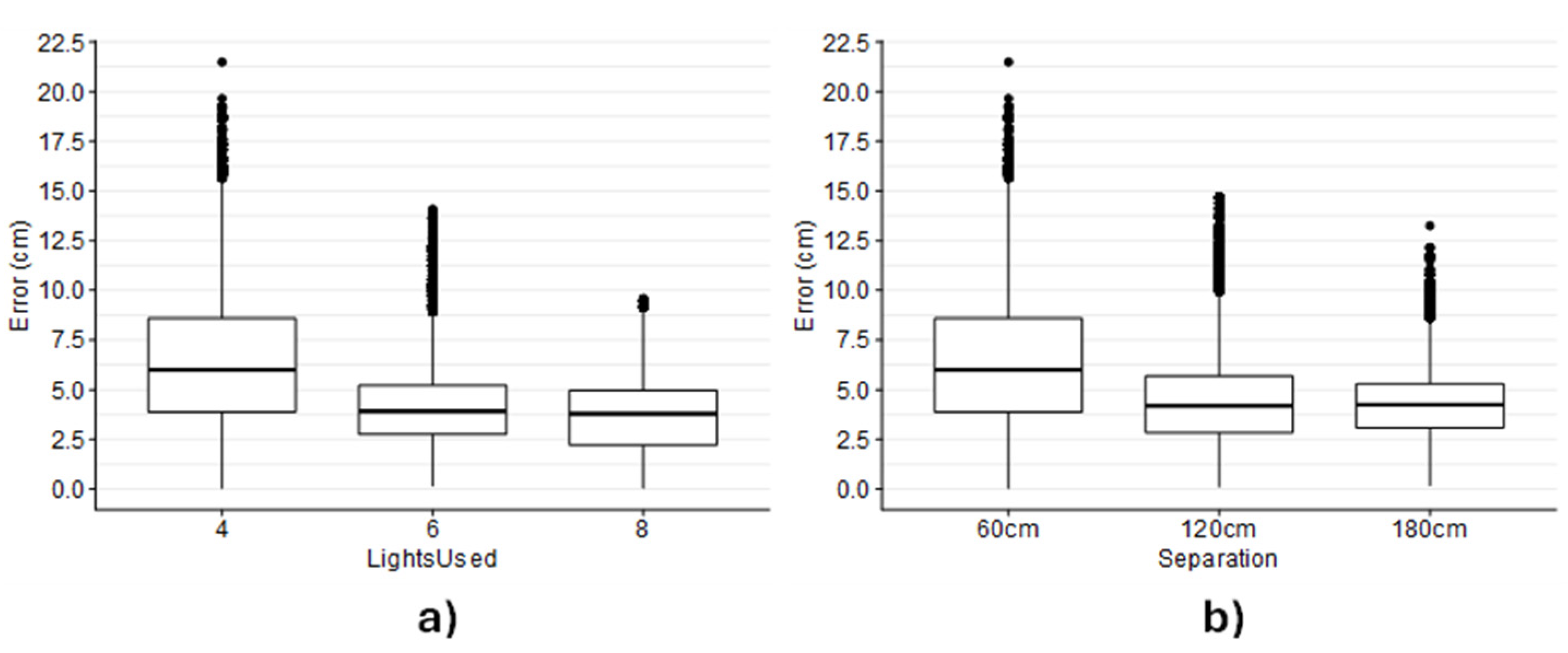
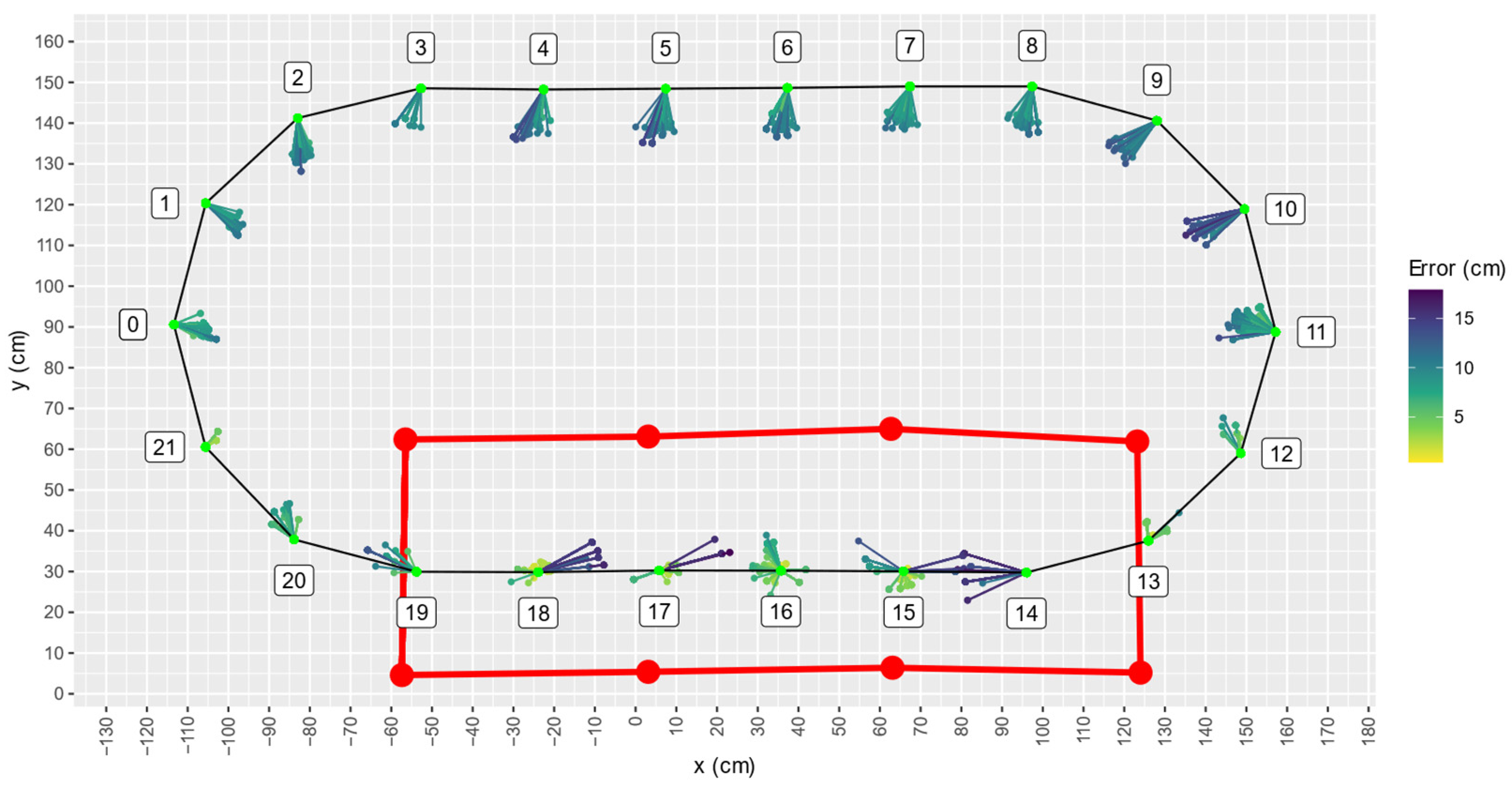
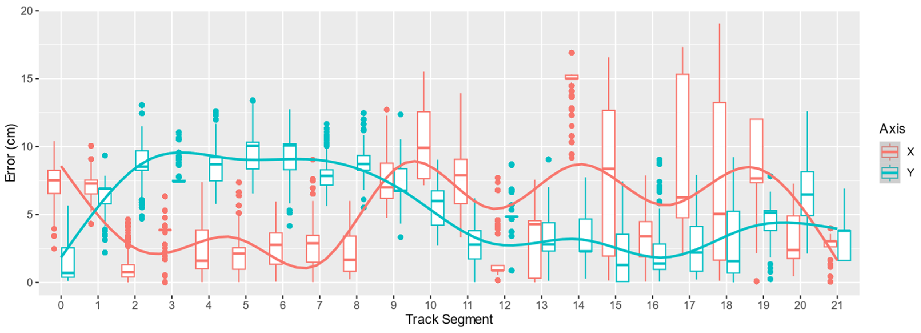
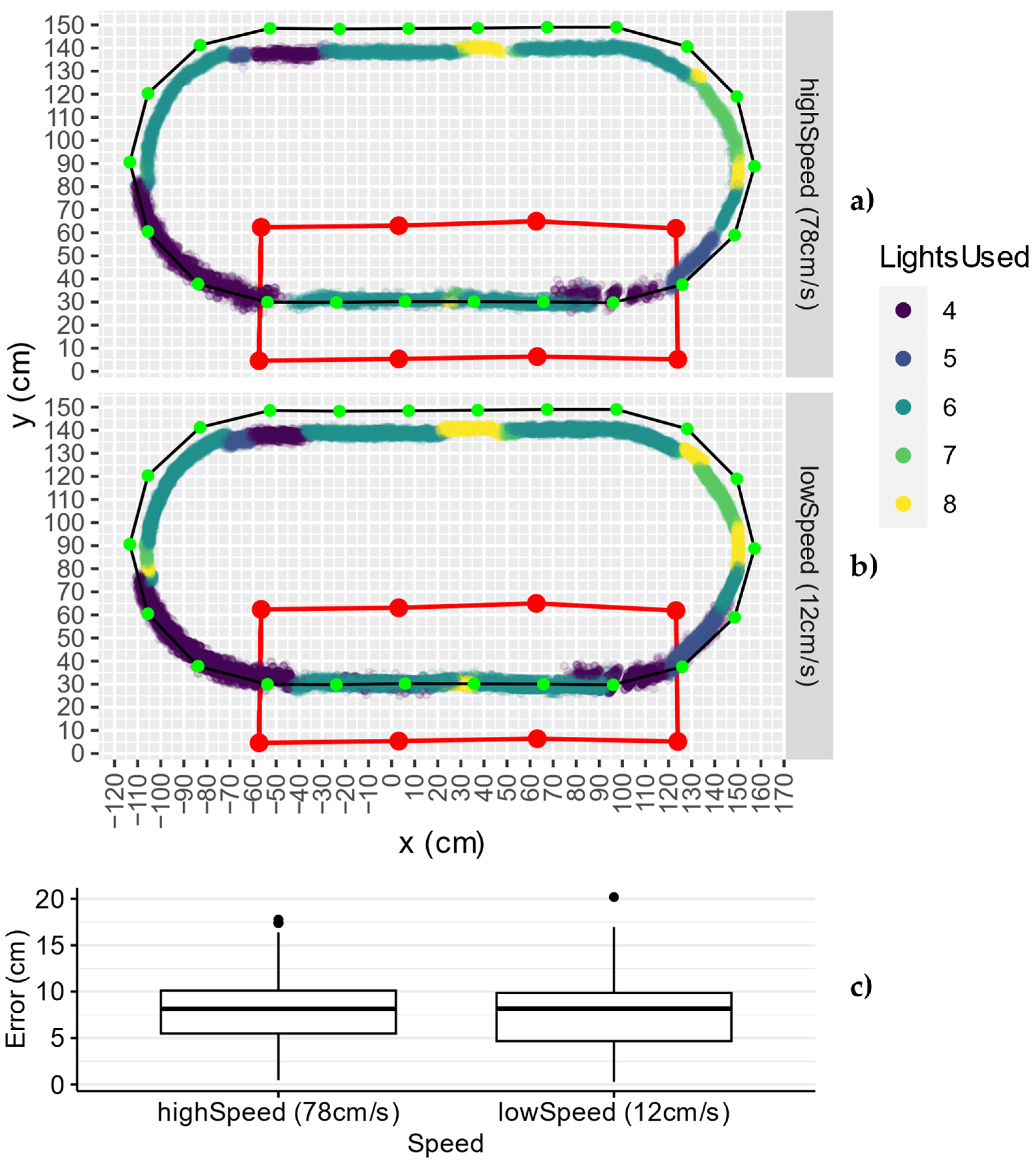
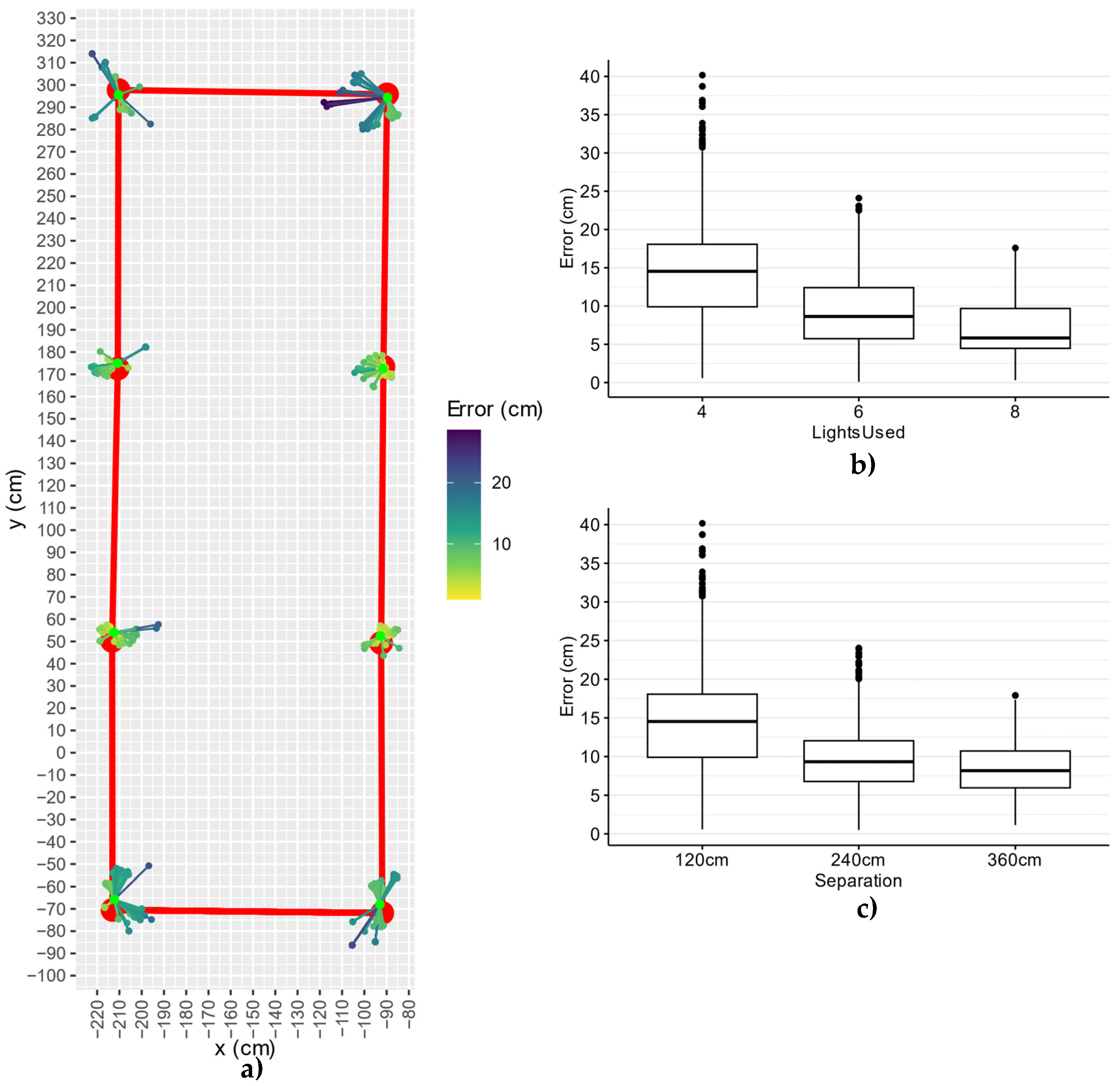
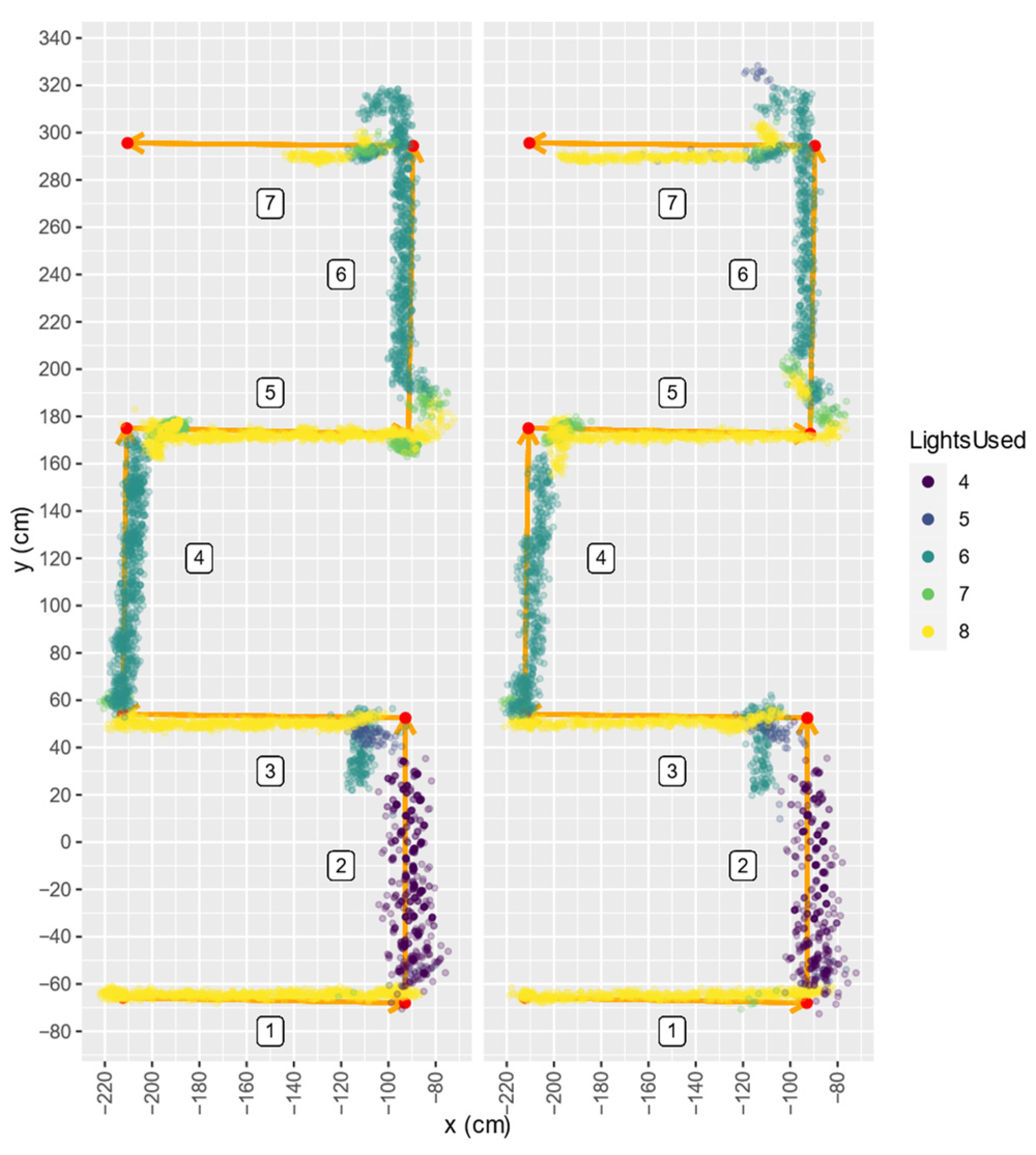
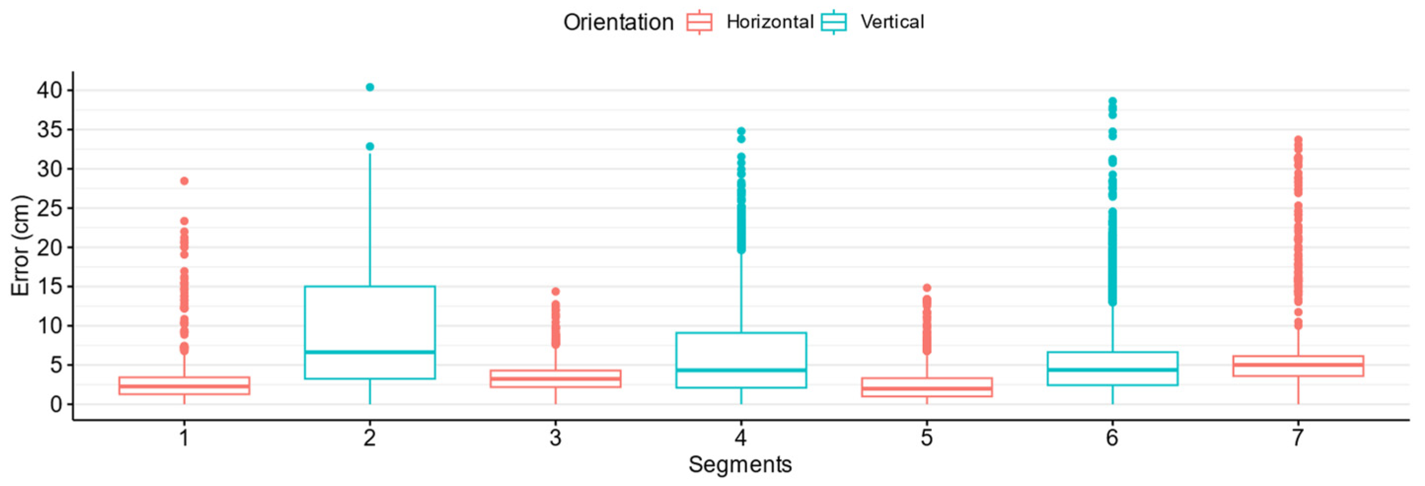

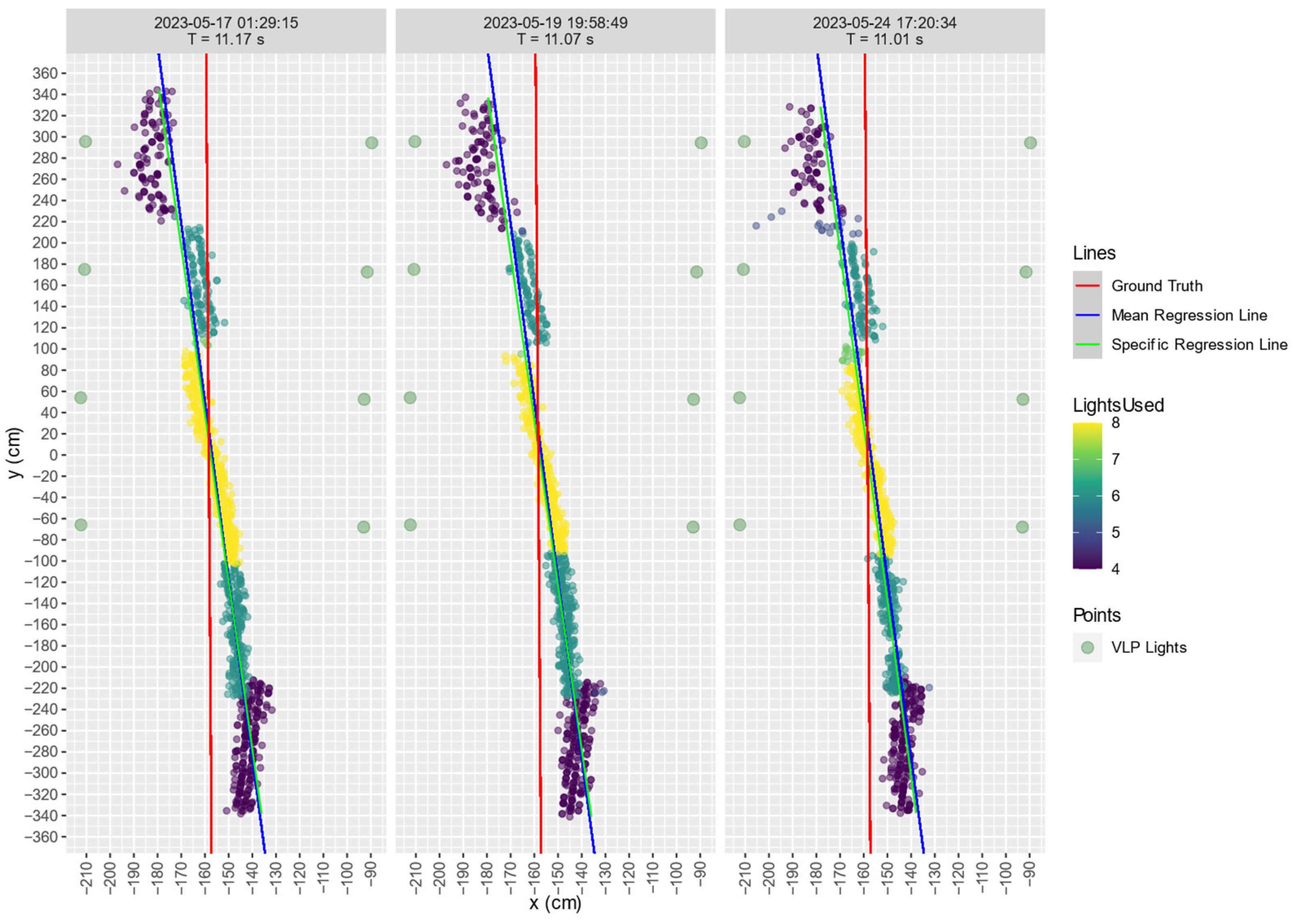
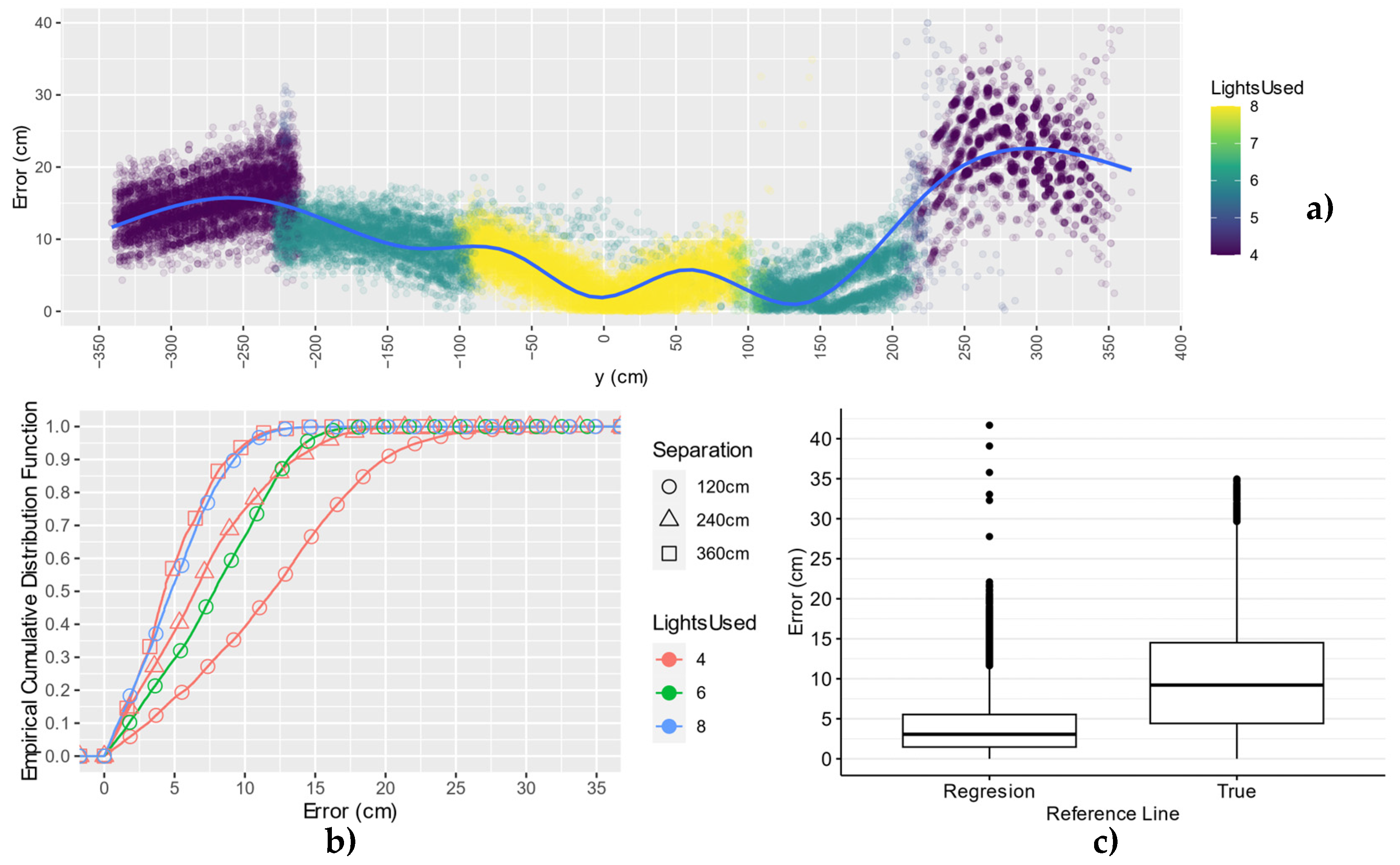
Disclaimer/Publisher’s Note: The statements, opinions and data contained in all publications are solely those of the individual author(s) and contributor(s) and not of MDPI and/or the editor(s). MDPI and/or the editor(s) disclaim responsibility for any injury to people or property resulting from any ideas, methods, instructions or products referred to in the content. |
© 2023 by the authors. Licensee MDPI, Basel, Switzerland. This article is an open access article distributed under the terms and conditions of the Creative Commons Attribution (CC BY) license (https://creativecommons.org/licenses/by/4.0/).