Abstract
The integrated circuit (IC) supply chain has become globalized, thereby inevitably introducing hardware Trojan (HT) threats during the design stage. To safeguard the integrity and security of ICs, many machine learning (ML)-based solutions have been proposed. However, most existing methods lack consideration of the integrity of HTs, thereby resulting in lower true negative rates (TNR) and true positive rate (TPRs). Therefore, to solve these problems, this paper presents a HT detection and diagnosis method for gate-level netlists (GLNs) based on ML and graph theory (GT). In this method, to address the issue of nonuniqueness in submodule partition schemes, the concept of “Maximum Single-Output Submodule (MSOS)” and a partition algorithm are introduced. In addition, to enhance the accuracy of HT diagnosis, we design an implant node search method named breadth-first comparison (BFC). With the support of the aforementioned techniques, we have completed experiments on HT detection and diagnosis. The HT implantation examples selected in this article are sourced from Trust-Hub. The experimental results demostrate the following: (1) The detection method proposed in this article, when detecting gate-level hardware trojans (GLHTs), achieves a TPR exceeding 95%, a TNR exceeding 37%, and F1 values exceeding 97%. Compared to existing methods, this method has improved the TNR for GLHTs by at least 25%. (2) The TPR for diagnosing GLHTs is consistently above 93%, and the TNR is 100%. Compared to existing methods, this method has achieved approximately a 4% improvement in the TPR and a 15% improvement in the TNR for GLHT diagnosis.
1. Introduction
Nowadays, the globalization of the integrated circuit (IC) industry chain has led to increased convenience, but it has also introduced vulnerabilities. These vulnerabilities can be exploited by attackers to implant a malicious module known as a hardware Trojan (HT) into an IC module [1,2]. Security attacks on the IC industry pose serious threats to people’s privacy and national security. Therefore, it is crucial to address this issue to ensure the continued reliability, security, and privacy protection of ICs.
The concept of HTs was first introduced in 2007 by Agrawal et al. [3]. In 2009, Jin et al. [4] specified the definition and composition of HTs. Subsequently, a series of HT detection methods have been presented one after another, such as side-channel analysis (SCA) [3,5,6,7], logic testing (LT) [8,9,10,11], formal verification (FV) [12,13,14], and gate-level feature extraction (GLFE) [15,16,17,18,19,20,21,22,23,24,25,26,27]. However, existing methods have several limitations. (1) GLFE needs golden GLN designs as reference. (2) SCA fails to detect small HTs because they are vulnerable to process variations and environmental noise. (3) LT requires a significant amount of time for design or enumeration. (4) For complex circuits, building an FV model is very challenging. Taking everything into account, we choose GLFE as the detection method and gate-level hardware trojan (GLHT) as the test HT. Firstly, GLFE tends to incorporate machine learning (ML) and has achieved good results. Secondly, GLHTs can be diagnosed through changes in the structure of the circuit diagram. However, most of the existing GLFE methods detect each node in the netlist directly, which can directly complete the diagnosis, but lack consideration for the integrity of the HTs, thus leading to the following problems: (1) Easily misjudging non-HT nodes with features similar to HT nodes, thereby resulting in low true negative rates (TNRs). (2) Easily missing HTs that only show relevant features on the whole, thereby resulting in low true positive rates (TPRs). (3) Some methods may partition submodules differently, thereby resulting in a decrease in the detection accuracy of the entire netlist.
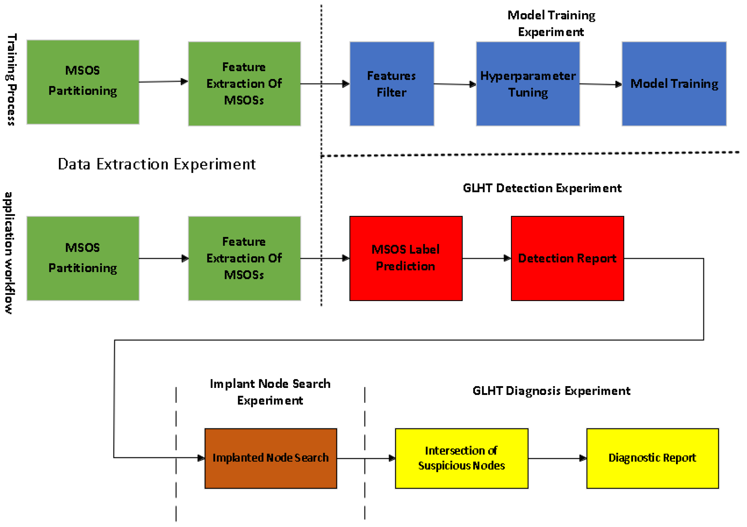
Based on the issues summarized above, this paper presents an HT detection and diagnosis method for gate-level netlists (GLNs) based on ML and graph theory (GT). The main process is as shown in Figure 1. Firstly, we partition the circuit diagram of a netlist into several maximum single-output submodules (MSOSs) and extract 24 HT-related features. Then, the chi-square tests and variance filtering methods are utilized to filter the features of each MSOS and adjust the hyperparameters until achieving the best balanced accuracy. We repeat this process for the sample to construct a specific supervised learning model. After that, we can use this learning model to make label predictions and obtain a detection report. Subsequently, by comparing the circuit diagram structures of the target netlist and the GLN, the additional nodes implanted in the target netlist can be accurately identified. Finally, we take the intersection of the nodes detected using ML and the additional implanted nodes found in the previous step to obtain the diagnosis report.
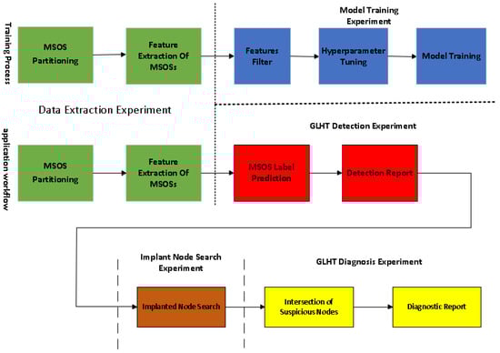
Figure 1.
Flow of the proposed HT detection and diagnosis method.
The contributions of this paper are summarized as follows:
- (1)
- An HT detection and diagnosis method for GLN based on ML and GT is proposed.
- (2)
- This paper, for the first time, proposes the concept and partition algorithm of MSOS to address the issue of nonunique submodule partition.
- (3)
- A total of 24 HT-related features are selected and extracted, including circuit diagram structure and static circuit attribute features.
- (4)
- We present a GT-based GLHT diagnosis method, which takes into account the comprehensiveness of HTs to fine-grain discover their locations.
- (5)
- In the implanted node search experiment, we propose the breadth-first comparison (BFC) algorithm, thereby increasing the diagnosis success rate.
The structure of this article is arranged as follows: Section 2 discusses the related work on GLFE. Section 3 elaborates on the research of GLHT detection methods based on ML. Section 4 presents the GT-based diagnosis method for GLHT. Section 5 presents the experimental process and analyzes the results. Section 6 makes a conclusion of this paper.
2. Related Work
GLFE is a type of method to complete nondestructive HT detection. Early GLFE methods directly compared the features with HT-related feature thresholds to complete HT detection. Waksman et al. [15] proposed a method for the functional analysis of HT structures by quantifying and evaluating the impact of inputs on outputs. Building on the study of Waksman et al., Fyrbiak et al. [16] proposed a reverse engineering (RE)-based method by introducing Boolean functions and graph structure neighborhood analysis. This approach reduced the detection error rate, but could only handle some less-frequent types of time-based HTs. Oya et al. [17] proposed a method to distinguish HTs by comparing scores calculated from HT templates and circuit simulation. This method could identify combinational or time-based HTs with relatively high accuracy. However, it was time-consuming due to the need for circuit simulation.
In recent years, there has been a trend to incorporate GLFE-based methods with ML to achieve better detection effects [22]. Hasegawa et al. [18,19,20] have successively employed supervised learning models such as the support vector machine (SVM) and random forest (RF) for GLHT detection. They have attempted various approaches to optimize supervised learning models with multiple HT features, thereby achieving high detection accuracy. However, the applicable GLHT types are too limited. Salmani et al. [21] applied unsupervised learning models within GLHT detection and proposed controllability and observability for hardware Trojan detection (COTD) method. This method, in conjunction with K-means and density-based spatial clustering of applications with noise (DBSCAN) algorithms, can effectively reconstruct and eliminate the entire HT module. Yan et al. [24] proposed a feature expansion algorithm based on the nearest neighbor unbalanced data classification algorithm, which improved the detection accuracy by increasing the sample feature set. Zhang et al. [25] proposed a mixed mode GLHT detection method based on the XGBoost algorithm. For the first time, the static and dynamic features were combined for multilevel HT detection, which effectively improved the detection accuracy. Li et al. [26] proposed an idea of using natural language processing to solve the problem of complex netlist structures that are difficult to analyze. They combined the netlist analysis methods of XGBoost, then converted the netlist into a sequence of logical structures and classified each logical structure according to its vector form, thus simplifying the detection process of GLHTs. Shi et al. [27] proposed a GLHT detection method based on a graph neural network. They used the graph sampling aggregation algorithm to learn the high-dimensional graph features and corresponding node features in the netlist, and they realized GLHT detection without using the golden netlist as a reference.
The combination of ML and GLFE can improve the accuracy and efficiency of HT detection, but it cannot diagnose HTs directly. At present, the diagnosis of HTs has gradually become the mainstream trend. Based on the study of Hasegawa et al., Du et al. [23] proposed an HT detection and diagnosis method based on “cone partition”, K-nearest neighbor (KNN), naive Bayes, and other supervised learning models. By changing the classification object from node to cone, the differences in the structures of centralized and distributed GLHTs were additionally considered. They partitioned the circuit into multiple cones and extracted the HT feature values of that method, and they then diagnosed the location of the HT circuits. Huang et al. [28] presented an HT detection and diagnosis method for GLNs based on different ML models. They classified all the circuit cones of the target GLN using different ML models; they then determined whether each circuit cone was HT-implanted through the label. This method had a good detection effect, but it could only roughly diagnose the location of the HT implantation.
With regard to detecting GLHTs, compared to earlier methods, current methods have achieved higher accuracy and broader applicability in both detection and diagnosis. However, most existing methods directly detect each node in the netlist. While this allows for direct diagnosis, it lacks a holistic consideration of HTs, thereby resulting in lower TPRs and TNRs. Additionally, certain methods may face the issue of nonuniqueness in the partition of the submodule, thereby affecting the overall detection accuracy of the entire netlist. The method we propose addresses these two issues, thereby leading to improved effectiveness in GLHT detection and diagnosis.
3. HT Detection Method for GLN Based on ML
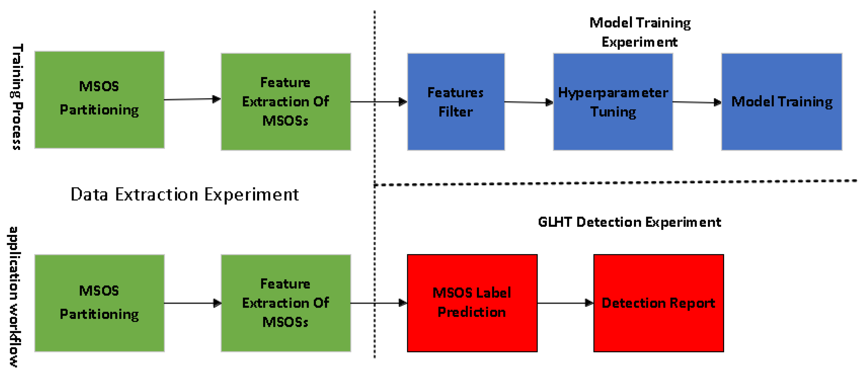
Aiming at the problem that the submodule partition scheme of the netlist is not unique, this paper proposes the concept and partition algorithm of the MSOS. A total of 24 HT-related features were chosen and extracted, including a circuit diagram structure and static circuit attribute features. On this basis, this paper studied an HT detection for GLNs based on ML models, and the main steps are shown in Figure 2:

Figure 2.
ML-based GLHT detection method.
- (1)
- MSOS partition: We partitioned the circuit diagram of the gate-level netlist into several MSOSs.
- (2)
- Feature extraction of MSOSs: We calculated and collected node information, and we then extracted HT-related features from the MSOSs.
- (3)
- Feature filter: We used chi-square tests and variance filtering methods to filter features of the MSOSs.
- (4)
- Model training: We trained a specific supervised learning model with optimized hyperparameters.
- (5)
- MSOS label prediction: We input the filtered features extracted from the MSOS into a specific supervised learning model for prediction.
- (6)
- Detection report: We reported whether the gate-level netlist contains an HT based on the labels.
3.1. MSOS Partition
In essence, the MSOS is a subcircuit diagram composed of several nodes and their corresponding units in the netlist. Specifically, considering the situation when the netlist contains or does not contain a ring structure, the MSOS is composed of several strongly connected components (SCCs) of nodes and their corresponding units.
Algorithm 1 is designed for the partition of each MSOS of the gate-level netlist. The search rule in step 10 can ensure that the MSOS has convergence, as well as a single-output and maximization at the same time. A simple example of MSOS partition is shown in Figure 3, in which the content in each rectangle box (because there is no ring structure, and one node corresponds to one SCC) is an MSOS.
| Algorithm 1: MSOS partition. |
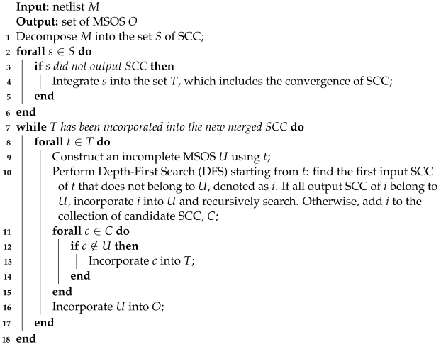 |
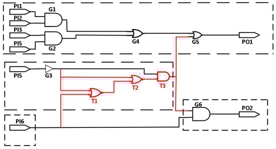
Figure 3.
Example of MSOS partition.
According to Figure 3 and Algorithm 1, it is not difficult to deduce that the partitioning of the MSOSs is similar to performing a DFS on all the SCCs. The only difference lies in step 10, where a single-output property check is required to add the input SCC (which can be achieved with the help of an SCC marking array). Therefore, the time complexity to partition MSOSs is proportional to the sum of the total number of SCCs, which is the total fan-in of the SCCs and the total fan-out of the SCCs. This is similar to O() in GT. Since the partitioning mainly involves creating independent marking arrays for each SCC, its space complexity is proportional to the square of the total number of SCCs, which is similar to O() in GT.
The GLHT detection method based on ML studied in this paper needs to solve the problem that the submodule partition scheme is not unique. At the same time, the MSOS partition is exactly unique, because there is only one scheme for any netlist to partition the MSOS. This is equivalent to there being no common SCC between any two different MSOSs. The partition of the MSOS is unique, which can be avoided when both submodules contain HT nodes. However, the influence of the HT nodes on the features is different, thereby resulting in a submodule being judged as “with” or “without” HTs. In addition, the feature extraction process of each MSOS will not affect each other, and this can be executed in parallel to improve efficiency.
3.2. Feature Extraction of MSOS
According to the analysis of other GLHT detection methods based on ML, the selection of HT-related features directly affects the detection accuracy. The relevant features of HTs selected by existing methods can be mainly partitioned into the following categories: circuit diagram structure, static circuit attributes, and dynamic circuit attributes.
For the MSOS, this paper selected 24 HT-related features of the circuit diagram structure and the static circuit attribute at the same time, and these features were mostly the maximum, minimum, average, and other statistical indicators. On the one hand, the changes in circuit structure features can show that additional modules are implanted in the MSOS, and the static circuit attribute features can further confirm whether the additional module contains HT nodes. On the other hand, the circuit structure- and static circuit attribute-related features can be obtained only using static analysis of the netlist, which takes less time. However, dynamic feature extraction requires providing specific test vectors, which is time-consuming and only effective for explicit HTs. Moreover, of all the circuit structure-related features, the 24 ones we selected have significant impacts on the feature values when an HT is implanted. Even with a slight modification to the MSOS, the values of the 24 HT-related feature will vary greatly in comparison to other features. Thus, we chose the 24 HT-related features from the circuit diagram structure and static circuit attributes, as shown in Table 1.

Table 1.
The 24 HT-related features.
3.2.1. Structure Class Features of Circuit Diagram
For each MSOS, the structure features of the 12 specific circuit diagrams selected in this paper are as follows:
- Node fan-in indicator: the maximum, minimum, and average value of the number of nodes entered by a node.
- Node fan-out indicator: the maximum, minimum, and average value of the number of nodes output by a node.
- SCC size indicator: the maximum, minimum, and average value of the number of nodes contained in the SCC to which the node belongs.
- Module fan-in: the number of input nodes when the entire MSOS is regarded as a single node.
- Module fan-out: the number of output nodes when the entire MSOS is regarded as a single node.
- Total number of nodes: the number of nodes contained in the MSOS.
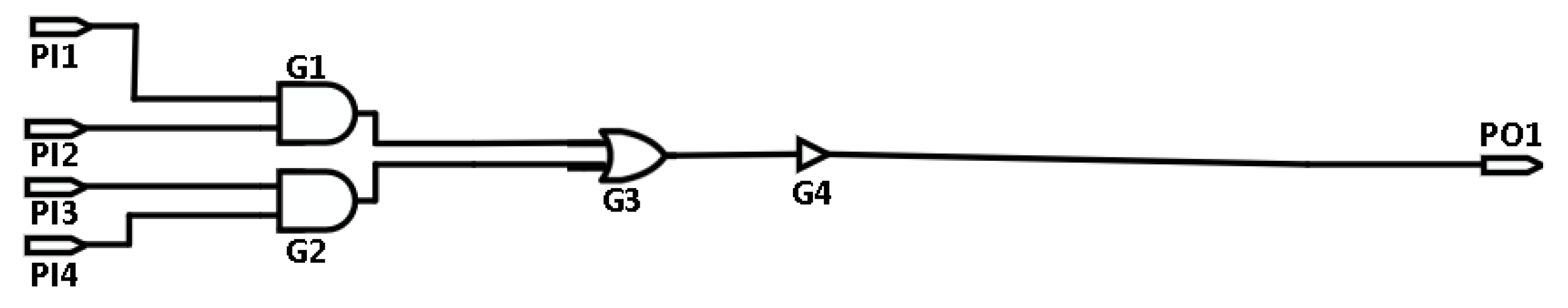
Figure 4 is an example of the MSOS without an HT implanted.
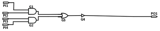
Figure 4.
An example of the MSOS without HT implanted.
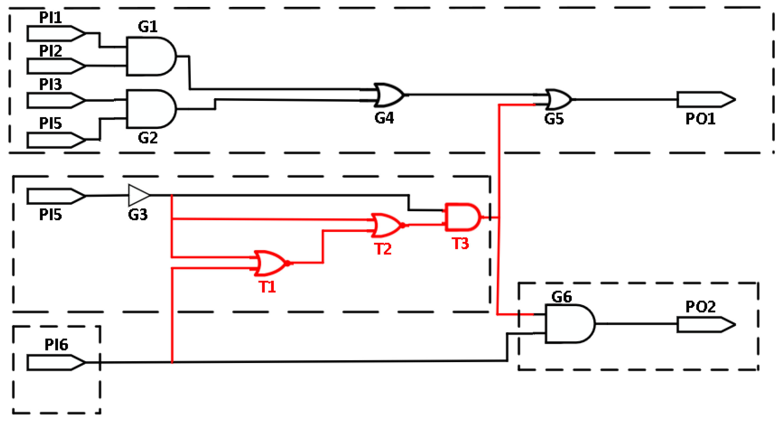
Figure 5 is an example of the entire HT implanted in an MSOS. The red portion is where the HT is implanted. The circuit diagram structure features underwent significant changes, such as average node fan-in and maximum node fan-out.
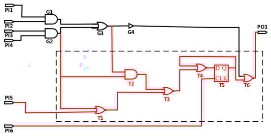
Figure 5.
An example of an HT with the complete implantation of an MSOS.
Because the circuit diagram structure features of Figure 4 were determined after parsing the netlist into the circuit diagram, it was only necessary to traverse all the nodes in the MSOS and produce statistics according to the corresponding conditions during extraction. The SCC size index needed to decompose the netlist circuit diagram first, and all the nodes in the same SCC needed to have the same SCC size; the module fan-in and module fan-out counted the number of input and output nodes, not the number of MSOSs of the input and output.
3.2.2. Attribute Class Features of Static Circuit
For each MSOS, the features of the 12 specific static circuit attributes selected in this paper are as follows:
- Combinational 0-controllability (CC0) index: the maximum, minimum, and average value of node CC0.
- Combinational 1-controllability (CC1) index of node combination 1: the maximum value, minimum value, and average value of node CC1.
- Combinational controllability (CC) index: the maximum, minimum, and average value of node CC.
- Combinational observability (CO) index of the nodes: the maximum, minimum, and average of node CO.
Compared with the circuit diagram structure feature, the static circuit attribute feature itself is more closely related to the HT, and it can be directly used to determine the existence of the HT. To extract the above static circuit attribute features, it is necessary to calculate the CC0, CC1, CC, and CO of all the nodes in the netlist in advance, and then count the CC0, CC1, CC, and CO of all the nodes in the MSOS.
3.3. Model Training and Label Prediction
After MSOS partitioning and feature extraction, variance filtering and chi-square tests were performed on the data set of the netlist to complete the feature selection. Then, the data texts of all the gate-level netlists were merged into the final data set. After that, we divided the final data set into a training data set and a testing data set. Hyperparameter tuning of the model was also performed using a crossvalidated grid parameter search method on the training data set. Finally, the ML models (i.e., KNN, RF, and the SVM) were obtained on the training data set using the selected hyperparameters.
The hyperparameter tuning results for the KNN, RF, and the SVM models are presented in Table 2, Table 3, and Table 4, respectively. The balanced accuracy (i.e., the arithmetic means of the TPRs and TNRs) serves as the metric for evaluating the predictive performance during crossvalidation. From these results, it can be observed that, with the optimal hyperparameters selected, the KNN, RF, and SVM models achieved balanced accuracies exceeding 80% on the training dataset.
Table 2.
The hyperparameter tuning results for the KNN model.
Table 3.
The hyperparameter tuning results for the RF model.
Table 4.
The hyperparameter tuning results for the SVM model.
After completing the training of the ML models, we used the testing data set to verify the trained KNN, RF, and SVM models to predict the label of each data set (corresponding to an MSOS).
4. HT Diagnosis Method for GLN Based on GT
The existing GLHT diagnosis methods are relatively small in number, and the diagnosis was generally completed by detecting the HT nodes in the netlist. The main drawback was still a lack of consideration for the overall HTs, thereby resulting in a low diagnosis accuracy problem. On this basis, this article studied a GLHT diagnosis method based on GT. As shown in Figure 6, the main steps are summarized as follows:
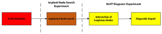
Figure 6.
GLHT diagnosis method based on GT.
- (1)
- GLHT detection: We used the GLHT detection method based on the ML models studied in this article.
- (2)
- Implanted node search: By comparing the circuit diagram structure of the target netlist and the GLN, we identified additional implanted nodes in the target netlist relative to the GLN.
- (3)
- Intersection of suspicious nodes (i.e., HT node localization): We intersected the nodes contained in the MSOS of the “HT” detected in step (1) and the nodes obtained from the implanted node search.
- (4)
- Diagnosis report: We reported the obtained node intersection as an HT node set.
Essentially, the netlist is a circuit diagram consisting of nodes and their corresponding cells. A netlist diagram can be further abstracted as a weighted directed graph: nodes are vertices, cells are edges, and the type of cells is the weight of the edge.
After abstracting the netlist circuit diagram into a weighted directed graph, the diagnosis of HTs at the gate-level can be transformed into a vertex search problem: finding the vertices in the graph that satisfy the features of the HTs. Compared with existing methods based on HT libraries and subgraph isomorphism, the GLHT diagnosis method studied in this paper avoids the need for further HT verification by intersecting the implanted node with an MSOS that has been detected as an “HT”.
4.1. Implanted Node Search Based on BFC
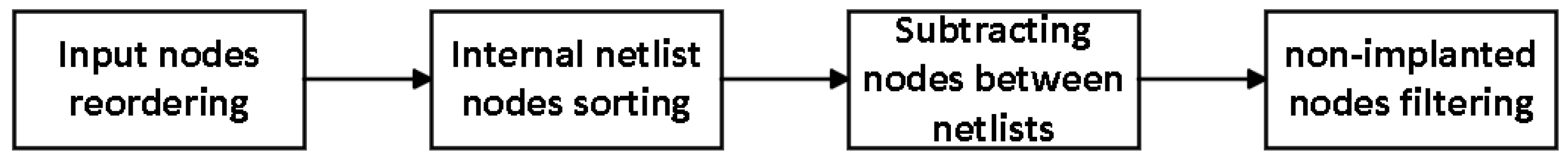
Firstly, we designed an algorithm that is independent of the specific circuit and compares the size relationship between any two nodes. Then, the node comparison algorithm was applied to sort and subtract the nodes in the target netlist and GLN to obtain candidate implantation nodes. Finally, we filtered out nonimplanted nodes from the candidate implanted nodes. Based on the above ideas, we designed an input-side BFC method and implemented an implanted node search algorithm based on the BFC method. As shown in Figure 7, the steps are summarized as follows:

Figure 7.
Implanted node search method based on BFC method.
- (1)
- Input nodes reordering: We determined the size relationships between nodes using an input-side BFC algorithm, and we then sorted the input nodes of all the nodes in the target netlist and GLN.
- (2)
- Internal netlist nodes sorting: We sorted the nodes of the target netlist and GLN.
- (3)
- Subtracting nodes between netlists: Sequentially, we compared the nodes in the target netlist and GLN to identify all the differing nodes, which were considered as candidate implanted points.
- (4)
- Nonimplanted nodes filtering: We filtered the nonimplanted nodes among the candidate implanted nodes based on the structure features and implantation ways of the GLHTs.
4.1.1. Input-Side BFC Algorithm
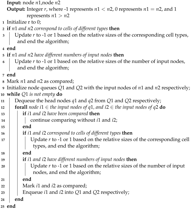
In a netlist, two nodes may be identical (requiring the same type of corresponding unit, number of input nodes, and number of output nodes), but the sequence of input-side BFC nodes and output-side BFC nodes of two nodes cannot be completely identical (requiring the nodes in both sequences to be exactly the same in dictionary order). Therefore, this article determined the size relationship of the nodes by comparing their input-side BFC node sequences, as shown in Algorithm 2.
This algorithm performs a BFC on the nodes. The number of iterations in the loop depends on the size of the queue and the comparisons between nodes. The overall time complexity reaches O() in the worst case, where N is the total number of input nodes. The overall space complexity of the algorithm is O(N) in the worst case, where N is the total number of input nodes.
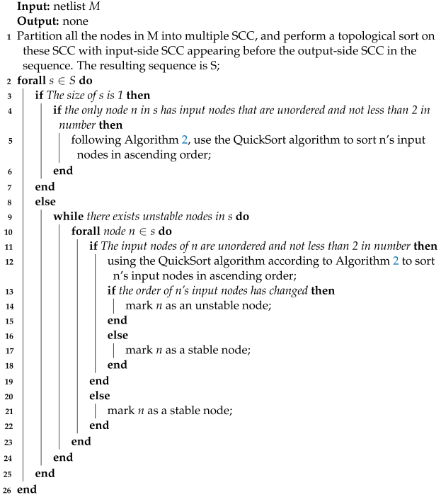
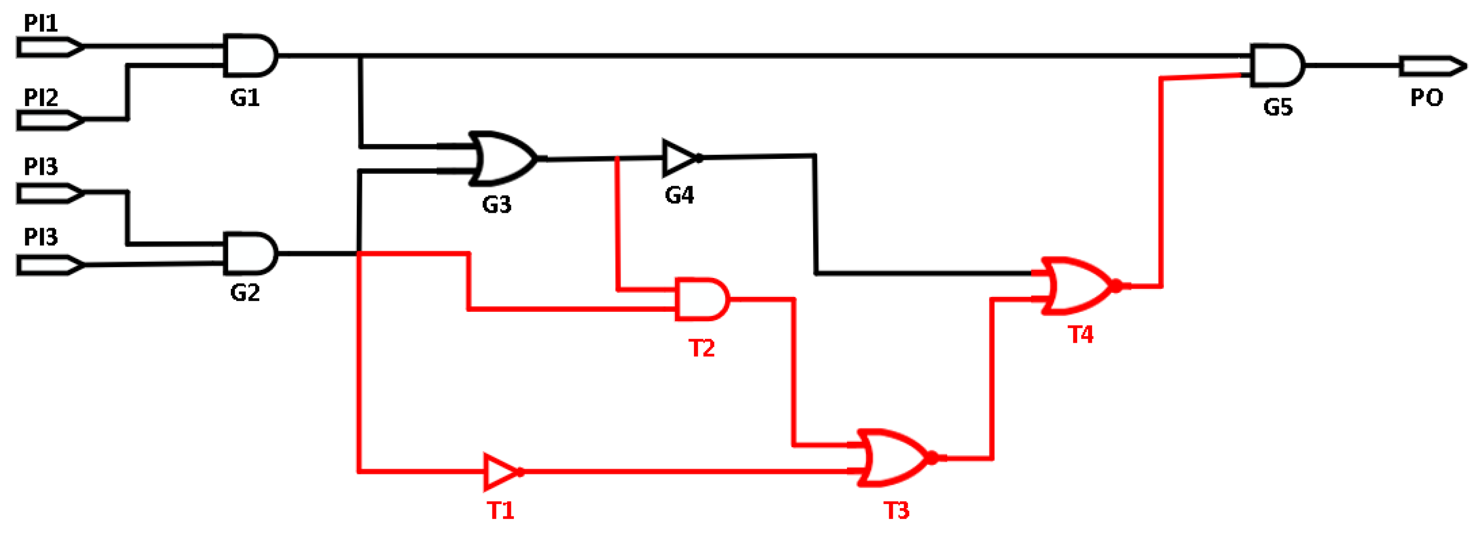
Figure 8 compares the nodes corresponding to the G1 and G6 units according to Algorithm 2. The nodes that have been compared in this figure are colored: green represents the same, while red or blue represents those that are different. It can be seen that, according to the breadth-first rule, when comparing the nodes corresponding to the G5 and G9 units, the nodes corresponding to the G1 unit were smaller because the former had a smaller number of input nodes.
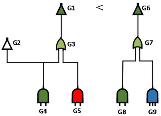
Figure 8.
An example of BFC on the input side.
4.1.2. Nonimplanted Node Filtering Algorithm
After using the input-side BFC algorithm for node sorting and subtraction, there were still some nonimplanted nodes among the candidate implanted nodes obtained. In order to filter out these nonimplanted nodes, this article mainly utilized the feature wherein the HTs only had a single load node (which was common in the HT implantation samples selected in this article, while the HTs in other samples could be split into sub-HTs of multiple single load nodes), as shown in Algorithm 3. This algorithm has a loop that runs for () iterations in the worst case. Each topological sorting iteration takes O) time, so the overall time complexity is O(). The space complexity is O().
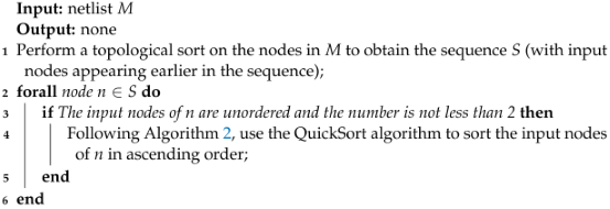
4.1.3. Input Node Reordering Algorithm
When comparing nodes, there may be an issue of input node disorder; in order to prevent the disorder of input nodes from interfering with node comparison, it is necessary to reorder the input nodes of all the nodes in the target netlist and GLN, as shown in Algorithm 4. In this algorithm, the time complexity of topological sorting is O(). The ‘for’ loop runs V times, and the time complexity of Algorithm 2 is O(). Therefore, the overall time complexity of the Algorithm 4 is O( + ). The space complexity is O(). However, topological sorting is only applicable to a directed acyclic graph, and there may be cyclic structures in the netlist circuit diagrams. Therefore, this article designed another input node reordering algorithm for the netlist containing circular structures, as shown in Algorithm 5. After analysis, the time complexity was determined to be O(), where V is the number of nodes in the netlist, E is the number of edges, and K is the number of SCCs. The space complexity is O().
| Algorithm 2: Input-side BFC algorithm. |
 |
4.2. Intersection of Suspicious Nodes
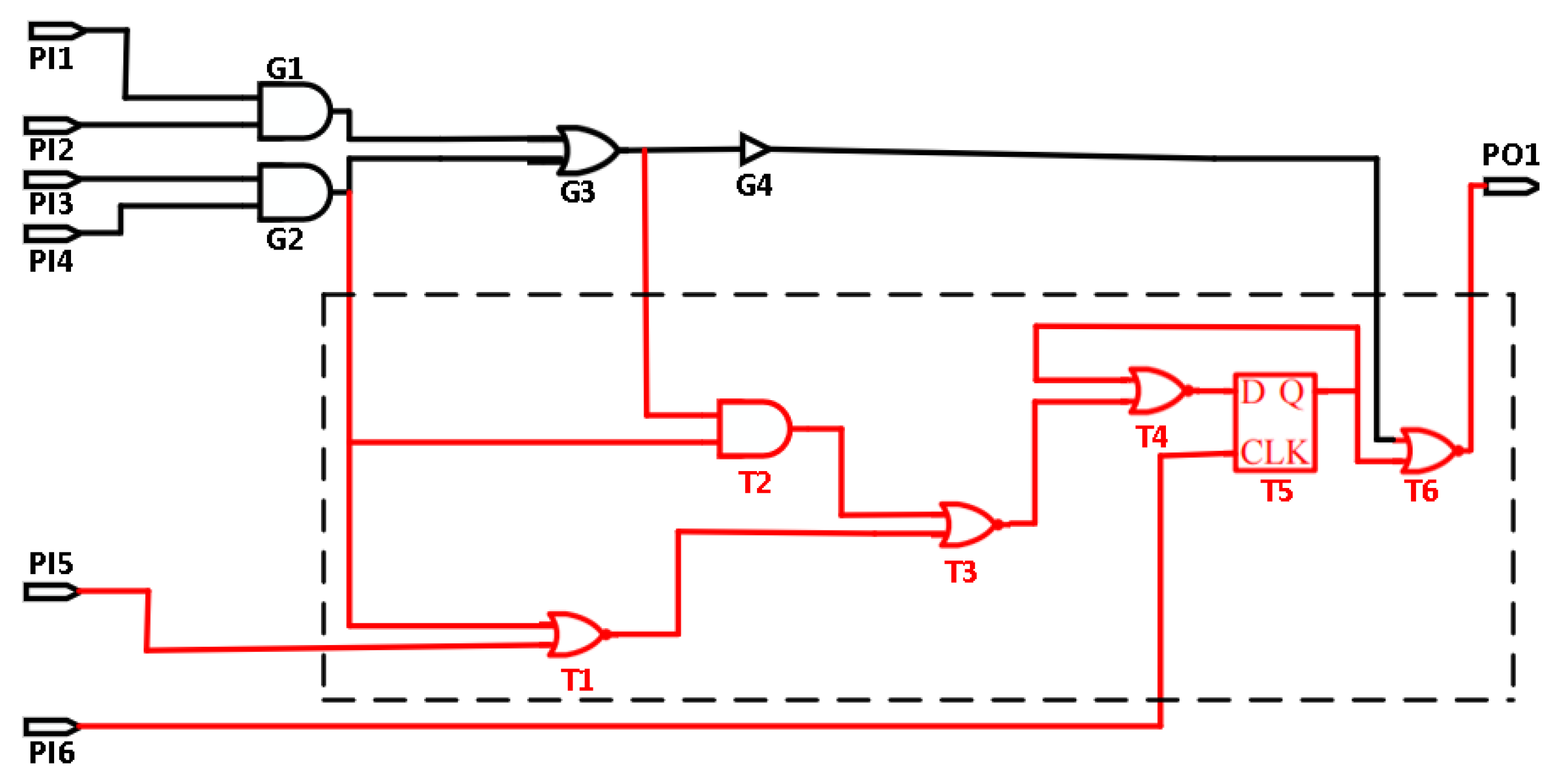
After the implant node search, we obtained the suspicious nodes (possibly HT nodes). Then, the intersection between the suspicious node and all the nodes of the MSOS detected in step (1) of Figure 6 was computed. At this point, we obtained the HT node set. It is necessary to know that if the target netlist is detected to contain HTs, then the nodes additionally implanted relative to the golden netlist must inherently contain nodes of the HTs. Therefore, the method described in this article searched for the nodes implanted in the target netlist relative to the golden netlist, and it then intersected them with the nodes in the MSOS. This process can avoid the requirement for further HT validation. Figure 9 presents an example of a netlist circuit diagram with a GLHT implanted. In particular, the red color represents the HT nodes obtained after the intersection.
| Algorithm 3: Filtering of nonimplant nodes. |
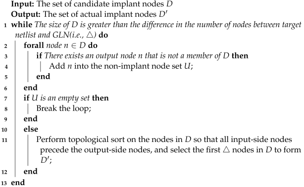 |
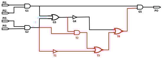
Figure 9.
Netlist circuit diagram with a GLHT implanted example.
| Algorithm 4: Filtering of nonimplant nodes. |
 |
| Algorithm 5: Filtering of nonimplant nodes. |
 |
5. Experiments and Results
This section describes the experimental procedure, results, and comparative analysis of our presented method.
5.1. Evaluation Measures
GLHT detection was used to determine whether there were HTs in the netlist. GLHT diagnosis was used to identify the HT nodes in the netlist. Therefore, the essence of GLHT detection and diagnosis is a binary classification problem, and they can be evaluated using relevant assessment metrics. The evaluation metrics for binary classification problems can be computed using the confusion matrix shown in Table 5. Several commonly used metrics are presented in Table 6.
Table 5.
Confusion matrix for binary classification.
Table 6.
Common binary classification evaluation metrics.
5.2. HT in GLN Detection Experiment
The CPU used in this experiment is the AMD Ryzen 5 3600, and the main frequency is 3.6 GHz. The memory is 16G DDR4, and the frequency is 3.2 GHz. In this paper, modern C++ was employed to construct and analyze the circuit netlist structure through independently designed graph structures and algorithms. To enhance the research efficiency, Python 3 was utilized, coupled with the open-source ML library “scikit-learn”, to implement the training and application of the supervised learning models.
The GLHT implantation example selected in this paper is from Trust-Hub and was generated using automated methods by the authors’ team mentioned in [29]. By varying the number of HTs, their functionalities, etc., a total of 914 GLHTs implantation instances were generated. According to whether the HT is a sequential circuit or a combinational circuit, these examples can be partitioned into two series: trit_tc series and trit_ts series. In this study, all the netlists were initially grouped based on their original design names and the number of HT instances. Then, within each group, the netlists were randomly split in a 7:3 ratio for training and testing purposes. Firstly, each netlist was partitioned into several MSOSs, and then 24 HT-related features corresponding to the MSOSs were extracted. Subsequently, these features were input into the ML models for label prediction. Here, we only selectively display the labels (as shown in Table 7), circuit structure-related features (as shown in Table 8), and static circuit attribute-related features (as shown in Table 9) of all the MSOSs in the s1423 and s1423_T002 netlists. The part marked in red means that the HT has been implanted.
Table 7.
Labels of all the MSOSs in the netlist of s1423 and s1423_T002.
Table 8.
Circuit structure features of all MSOSs in the s1423 and s1423_T002 netlists.
Table 9.
Static circuit attribute features of all MSOSs in the s1423 and s1423_T002 netlists.
The “number” refers to a specific MSOS. Based on the tables above, it can be concluded that, compared to the s1423 netlist, the fifth MSOS of the s1423_T002 netlist experienced changes in some features because it contained the entire HT implant. On the other hand, the other MSOSs, which were not implanted with any HT nodes, had all of their features remain unchanged. This proves the effectiveness of our method.
For all the testing data set, the detection results of the HTs in the MSOSs are shown in Table 10. According to the analysis of these results, the detection effects of the KNN, RF, and SVM models were good enough, the RF model was the best, and the KNN model was the second best. In terms of HT detection in the netlist, all the models had TPRs over 95%, TNRs over 37%, and F1 scores over 97%.
Table 10.
Detection results of HTs in MSOSs.
The comparative object selected in this article was the method studied in [23]. Compared with the other GLHT detection-based ML methods, this method not only had better detection performance, but was also closer to the method studied in this article. The GLHT detection results of the method in [23] are shown in Table 11.
Table 11.
Comparison of hardware Trojan detection results.
By analyzing Table 11, we can obtain the comparison results of the GLHT detection performance outcomes between the method proposed in this paper and the method proposed in [23] when using the KNN, RF, and SVM models. Although the method described in this paper took more time for detection (on the one hand, the number of MSOSs in the same netlist was generally much greater than the number of cones; on the other hand, the feature dimension of the MSOS was three times that of the cone), the overall detection performance was better, especially with a TNR improvement of at least 25%.
For another comparative experiment, we chose [28], which implemented GLHT detection using ML with different models and achieved good results. Table 12 shows the comparative detection results; it is evident that, although the TNR in this article was lower compared to [28], the F1 score generally tended to be higher than that of [28]. The results suggest that the model has a good trade-off between correctly identifying positive instances (precision) and capturing all positive instances (recall).
Table 12.
The GLHT detection results in this article and [28].
5.3. HT in GLN Diagnosis Experiment
The results of the GLHT diagnosis for all test netlists are shown in Table 13. It can be seen from the analysis of the results that using the KNN, RF, or SVM models, coupled with the implanted node search method based on BFC, could achieve average TPRs exceeding 93% and average TNRs of 100% in diagnosing HT nodes in the netlists.
Table 13.
Results of GLHT diagnosis.
For comparison with the GLHT diagnosis results, this study selected a method proposed in [30], which uses adversarial learning (called “R-HTDetector”). Compared to the other methods, this method is not only the latest research achievement of the pioneering team that applied ML models to GLHT detection and diagnosis, but it also achieves significant improvements in accuracy and applicability by conducting adversarial learning on automatically generated GLHT variants. For the testing netlists selected by the R-HTDetector method, the GLHT diagnosis results using the R-HTDetector method and the method proposed in this article are shown in Table 14. From the analysis of Table 14, it can be observed that, compared with the R-HTDetector method, the method proposed in this paper achieved an improvement of approximately 4% and 15% in the average TPR and TNR values of the GLHT diagnosis, respectively.
Table 14.
GLHT diagnosis results of R-HTDetector and the method described in this article.
For another comparative experiment, we chose [23,28], as shown in Table 15. In [23], the authors partitioned the circuit into multiple sectors and extracted the HT feature values of those sectors to complete the diagnosis. In [28], the authors completed the diagnosis by obtaining the primary output of the netlist. Although they could complete the diagnosis, it was not accurate enough. Our method accurately located the location of the HT by searching each node.
Table 15.
Comparison of GLHT diagnostic results.
6. Conclusions
This paper focused on an HT detection and diagnosis method for GLN based on ML and GT. To address the issue of nonunique submodule partition schemes in netlists, we proposed the concept and partition algorithm of the MSOS, and we extracted 24 HT-related features based on the circuit structure and static circuit attributes of the MSOS. We conducted data extraction, model training, and GLHT detection experiments on the trit_tc and trit_ts series of the GLHT implantation examples. Table 11 and Table 12 show that our method has good detection performance in GLHT detection, and this was improved significantly compared to the existing methods. In additional, to improve the accuracy of GLHT diagnosis, we proposed an implant node search method based on BFC. Table 14 and Table 15 also show that our proposed approach has good diagnosis performance for GLHTs and this was improved significantly compared to the existing methods. However, there are some drawbacks to our method, such as the inability to avoid the reference to golden GLN designs. We will try to solve this problem in the future work.
Author Contributions
Conceptualization, Z.L., L.X. and Z.H.; methodology, J.W., G.Z., Z.H., C.X. and X.L.; software, J.W., H.G., G.Z., C.X., Z.H. and X.L.; validation, J.W., Z.H., Z.L., H.G. and X.L.; writing—original draft preparation, J.W., L.X., G.Z. and Z.H.; writing—review and editing, J.W., Z.H., Z.L., X.L. and L.X.; supervision, Z.H., L.X. and H.G.; project administration, Z.H., L.X., X.L. and H.G.; funding acquisition, Z.H., L.X., X.L. and H.G. All authors have read and agreed to the published version of the manuscript.
Funding
This work was supported in part by the National Natural Science Foundation of China under Grant 61972302, in part by the Guangzhou Municipal Science and Technology Project under Grant SL2022A04J00404, in part by the Fundamental Research Funds for the Central Universities under Grant XJS220306, in part by the Natural Science Basic Research Program of Shaanxi under Grant 2022JQ-680, and in part by the Key Laboratory of Smart Human Computer Interaction and Wearable Technology of Shaanxi Province. Research project on Integrated Real Security System of sea, land, air and space: 2022-KY-0031.
Data Availability Statement
Data is unavailable due to privacy or ethical restrictions.
Acknowledgments
The authors would like to thank the editors and reviewers for their contributions to our manuscript.
Conflicts of Interest
Author Junjie Wang and Lihui Xu was employed by the company CNNC Intelligent Security Technology Co., Ltd. Author Changjian Xie was employed by the company Zhejiang Raina Tech. Inc. The remaining authors declare that the research was conducted in the absence of any commercial or financial relationships that could be construed as a potential conflict of interest.
References
- Huang, Z.; Wang, Q.; Chen, Y.; Jiang, X. A survey on machine learning against hardware Trojan attacks: Recent advances and challenges. IEEE Access 2020, 8, 10796–10826. [Google Scholar] [CrossRef]
- Salmani, H.; Tehranipoor, M. Digital Circuit Vulnerabilities to Hardware Trojans. In Hardware IP Security and Trust; Mishra, P., Bhunia, S., Tehranipoor, M., Eds.; Springer: Cham, Sitzerland, 2017. [Google Scholar]
- Agrawal, D.; Baktir, S.; Karakoyunlu, D.; Rohatgi, P. Trojan detection using IC fingerprinting. In Proceedings of the 2007 IEEE Symposium on Security and Privacy (SP ’07), Berkeley, CA, USA, 20–23 May 2007; pp. 296–310. [Google Scholar]
- Jin, Y.; Kupp, N.; Makris, Y. Experiences in hardware trojan design and implementation. In Proceedings of the 2009 IEEE International Workshop on Hardware-Oriented Security and Trust, San Francisco, CA, USA, 27–27 July 2009; pp. 50–57. [Google Scholar]
- Salmani, H.; Tehranipoor, M.; Plusquellic, J. A novel technique for improving hardware trojan detection and reducing trojan activation time. IEEE Trans. Very Large Scale Integr. (Vlsi) Syst. 2012, 20, 112–125. [Google Scholar] [CrossRef]
- He, J.; Zhao, Y.; Guo, X.; Jin, Y. Hardware trojan detection through chip-free electromagnetic side-channel statistical analysis. IEEE Trans. Very Large Scale Integr. (Vlsi) Syst. 2017, 25, 2939–2948. [Google Scholar] [CrossRef]
- Faezi, S.; Yasaei, R.; Barua, A.; Al Faruque, M.A. Brain-inspired golden chip free hardware trojan detection. IEEE Trans. Inf. Forensics Secur. 2017, 16, 2697–2708. [Google Scholar] [CrossRef]
- Dupuis, S.; Flottes, M.-L.; Di Natale, G.; Rouzeyre, B. Protection against hardware trojans with logic testing: Proposed solutions and challenges ahead. IEEE Des. Test 2018, 35, 73–90. [Google Scholar] [CrossRef]
- Wolff, F.; Papachristou, C.; Bhunia, S.; Chakraborty, R.S. Towards trojan-free trusted ICs: Problem analysis and detection scheme. In Proceedings of the 2008 Design, Automation and Test in Europe, Munich, Germany, 10–14 March 2008; pp. 1362–1365. [Google Scholar]
- Saha, S.; Chakraborty, R.S.; Nuthakki, S.S.; Anshul; Mukhopadhyay, D. Improved test pattern generation for hardware trojan detection using genetic algorithm and boolean satisfiability. In Proceedings of the Cryptographic Hardware and Embedded Systems–CHES 2015, Saint-Malo, France, 13–16 September 2015; Springer: Berlin/Heidelberg, Germany, 2015; pp. 577–596. [Google Scholar]
- Kampel, L.; Kitsos, P.; Simos, D.E. Locating hardware trojans using combinatorial testing for cryptographic circuits. IEEE Access 2022, 10, 18787–18806. [Google Scholar] [CrossRef]
- Zhang, X.; Tehranipoor, M. Case study: Detecting hardware trojans in third-party digital IP cores. In Proceedings of the 2011 IEEE International Symposium on Hardware-Oriented Security and Trust, San Diego, CA, USA, 5–6 June 2011; pp. 67–70. [Google Scholar]
- He, J.; Guo, X.; Meade, T.; Dutta, R.G.; Zhao, Y.; Jin, Y. SoC interconnection protection through formal verification. Integration 2019, 64, 143–151. [Google Scholar] [CrossRef]
- Qin, M.; Hu, W.; Wang, X.; Mu, D.; Mao, B. Theorem proof based gate-level information flow tracking for hardware security verification. Comput. Secur. 2019, 85, 225–239. [Google Scholar] [CrossRef]
- Waksman, A.; Suozzo, M.; Sethumadhavan, S. FANCI: Identification of stealthy malicious logic using boolean functional analysis. In Proceedings of the ACM SIGSAC Conference on Computer & Communications Security, Berlin, Germany, 4–8 November 2013. [Google Scholar]
- Fyrbiak, M.; Wallat, S.; Swierczynski, P.; Hoffmann, M.; Hoppach, S.; Wilhelm, M.; Weidlich, T.; Tessier, R.; Paar, C. HAL–The missing piece of the puzzle for hardware reverse engineering, trojan detection and insertion. IEEE Trans. Dependable Secur. Comput. 2019, 16, 498–510. [Google Scholar] [CrossRef]
- Oya, M.; Shi, Y.; Yanagisawa, M.; Togawa, N. A score-based classification method for identifying hardware trojans at gate-level netlists. In Proceedings of the Design, Automation & Test in Europe Conference & Exhibition (DATE), Grenoble, France, 9–13 March 2015; pp. 465–470. [Google Scholar]
- Hasegawa, K.; Oya, M.; Yanagisawa, M.; Togawa, N. Hardware trojans classification for gate-level netlists based on machine learning. In In Proceedings of the IEEE 22nd International Symposium on On-Line Testing and Robust System Design (IOLTS), Sant Feliu de Guixols, Spain, 4–6 July 2016; pp. 203–206. [Google Scholar]
- Hasegawa, K.; Yanagisawa, M.; Togawa, N. Hardware trojans classification for gate-level netlists using multi-layer neural networks. In Proceedings of the IEEE 23rd International Symposium on On-Line Testing and Robust System Design (IOLTS), Thessaloniki, Greece, 3–5 July 2017; pp. 227–232. [Google Scholar]
- Hasegawa, K.; Yanagisawa, M.; Togawa, N. Trojan-feature extraction at gate-level netlists and its application to hardware-trojan detection using random forest classifier. In Proceedings of the IEEE International Symposium on Circuits and Systems (ISCAS), Baltimore, MD, USA, 28–31 May 2017; pp. 1–4. [Google Scholar]
- Salmani, H. Cotd: Reference-free hardware trojan detection and recovery based on controllability and observability in gate-level netlist. IEEE Trans. Inf. Forensics Secur. 2017, 12, 338–350. [Google Scholar] [CrossRef]
- Zhao, J.; Shi, G. Survey on the research progress of hardware trojans. J. Inf. Secur. 2017, 2, 17. [Google Scholar]
- Du, M. A HT Detection and Diagnosis Method for Gate-level Netlists based on Machine Learning. Ph.D. Dissertation, Xi’an University of Electronic Science and Technology, Xi’an, China, 2021. [Google Scholar]
- Yanjian, Y.; Conghui, Z.; Yanjiang, L. Hardware Trojan Detection Technology Based on Multidimensional Structural Features. J. Electron. Inf. Technol. 2021, 43, 2128. [Google Scholar]
- Ma, S.; Liu, Y.; Wu, Y.; Zhang, S.; Zhang, Y.; Wang, D. Hybrid Mode Gate-Level Hardware Trojan Detection Method Based on XGBoost. J. Electron. Inf. Technol. 2021, 43, 3050. [Google Scholar]
- Xin, L.; Haiming, L.; Jian, M. Hardware Trojan Detection Based on Circuit Structure Analysis Using Integrated Model. Microelectron. Comput. 2021, 38, 80–86. [Google Scholar]
- Shi, J.; Wen, C.; Liu, H.; Wang, Z.; Zhang, S.; Ma, P.; Li, K. Hardware Trojan Detection for Gate-level Netlists Based on Graph Neural Network. J. Electron. Inf. Technol. 2023, 45, 3253–3262. [Google Scholar]
- Huang, Z.; Xie, C.J.; Li, Z.Y.; Du, M.F.; Wang, Q. A hardware trojan detection and diagnosis method for gate-level netlists based on different machine learning algorithms. J. Circuits Syst. Comput. 2022, 31, 2250135:1–2250135:25. [Google Scholar] [CrossRef]
- Cruz, J.; Huang, Y.; Mishra, P.; Bhunia, S. An automated configurable trojan insertion framework for dynamic trust benchmarks. In Proceedings of the Design, Automation & Test in Europe Conference & Exhibition (DATE), Dresden, Germany, 19–23 March 2018; pp. 1598–1603. [Google Scholar]
- Hasegawa, K.; Hidano, S.; Nozawa, K.; Kiyomoto, S.; Togawa, N. R-htdetector: Robust hardware-trojan detection based on adversarial training. IEEE Trans. Comput. 2023, 72, 333–345. [Google Scholar] [CrossRef]


Disclaimer/Publisher’s Note: The statements, opinions and data contained in all publications are solely those of the individual author(s) and contributor(s) and not of MDPI and/or the editor(s). MDPI and/or the editor(s) disclaim responsibility for any injury to people or property resulting from any ideas, methods, instructions or products referred to in the content. |
© 2023 by the authors. Licensee MDPI, Basel, Switzerland. This article is an open access article distributed under the terms and conditions of the Creative Commons Attribution (CC BY) license (https://creativecommons.org/licenses/by/4.0/).