Abstract
Clustering is an important means to solve the poor scalability of aeronautical ad hoc networks (AANET). To improve the stability and performance of AANET and avoid unnecessary waste of resources caused by civil aircraft in communication, we proposed a zero-overhead clustering algorithm according to the real-time position of the aircraft based on the known trajectory. Firstly, the route and trajectory models are used to obtain geographical coordinates by the aircraft positioning algorithm. On this basis, the geographical cluster and cluster head region are divided in order to complete the cluster setting. Considering the aircraft maintenance cluster generation time updates, we use the communication sub-cluster generation algorithm to control the size of the cluster, and also, the flexibility of cluster hops is guaranteed by the subsidiary cluster members. The continuity of communication and the scalability of the cluster are maintained by the gateway node, thereby forming a network structure and increasing the stability of clusters. Finally, the actual route data are used to simulate the performance of the algorithm. The experimental and analytical results show that clustering and maintenance of the algorithm have zero overhead. Additionally, compared with the traditional algorithm, our proposed method can maintain a reasonable number of clusters, reduce the frequency of cluster head replacement, reduce the number of cluster members entering and leaving the cluster and avoid the loss of control of cluster heads to cluster members. So, it has important application value in the field of civil aviation.
1. Introduction
Aviation ad hoc networks (AANET) involve the expansion and application of a mobile ad hoc network in the aviation field. The establishment of AANET by civil aircraft can realize direct communication between aircraft, allowing them to send real-time status information and air perception information to each other so as to improve flight safety, facilitate traffic control, share information, provide Internet services for passengers and other purposes [1]. However, the establishment of AANET will pose new difficulties for routing protocol [2], Qos guarantee [3] and scalability; in addition, the connectivity problem of the aviation ad hoc network will also affect the networking mode and route selection [4]. To solve these problems, researchers proposed a way to divide the network into groups, namely, using clustering algorithms. The use of a clustering structure can greatly improve routing performance and solve problems such as a limited network scale, thereby improving network performance and efficiency [5].
Traditional clustering algorithms such as minimum ID [6] and maximum connectivity [7] have studied the establishment of clusters from multiple perspectives such as energy saving and weight setting. Vatambeti [8] proposes a new method of creating nodes using star topology, which can effectively predict link obstacles in a network and improve the lifetime of nodes. Bilen [9] proposes a customized K-means algorithm, which takes into account the location (latitude and longitude), direction, angle, altitude and other information in the clustering process to achieve AANET cluster stability. Based on the density clustering algorithm, Shahbazi [10] proposes a new AANET adaptive cluster head selection algorithm, which improves the stability of air-to-air links, increases the lifetime of cluster heads and reduces the rate of change. However, the influence of external environmental factors such as turbulence were not taken into account. Wang [11] selects cluster heads from the perspective of minimizing the energy consumption of the network and the algorithm better balances the energy consumption and improves the energy efficiency, thus prolonging the lifetime of the network. But this algorithm is only suitable for fixed networks. Chang [12] proposes an algorithm for selecting cluster heads and allocating remaining nodes based on node distribution density, which realizes rapid selection of cluster heads and rapid division of clusters. However, the time complexity and time-consuming nature of this algorithm are relatively high. Ahmad [13] proposes a clustering algorithm that can adapt to the dynamic and rapid changes of topology and can form equilibrium and stable clusters. However, whether it can be applied to an aviation ad hoc network environment still needs further research. Zhang [14] uses an analytic hierarchy process to select super cluster heads from cluster heads by integrating node energy, node centrality, node degree and other factors. However, civil aircraft do not need to consider the residual energy, power level and other parameters.
The civil aviation ad hoc network has the following characteristics which are different from conventional ad hoc networks:
- (a)
- The predictability of movement. The takeoff and landing of civil aircraft or even the flight trajectory, flight direction and speed are strictly implemented in accordance with regulations, and the flight path of the same route is basically unchanged.
- (b)
- The high speed of aircraft motion. The speed of aircraft is usually 500–1000 km/h, and the high-speed movement of nodes will cause rapid changes in network topology, which directly affects the performance of MAC protocol, routing protocol and others.
- (c)
- Large-scale distribution of scenes. The geographical range of aircraft distribution is wide, such as the ocean, continent, desert and other areas without ground transfer stations.
- (d)
- Unlimited energy of node. The flight time is usually a few hours, and the aircraft will provide enough energy for communication, so the effect of node energy is ignored.
The design goal of the clustering algorithm should consider the specific practical demand. However, the traditional clustering algorithm does not consider the characteristics of civil aviation, so it may cause unnecessary communication overhead and resource waste, or even lead to network paralysis. Although some algorithms combine the characteristics of civil aviation, Ergenç [15] proposes a new clustering algorithm based on reliability, that is, it focuses on the reliability of the whole cluster, rather than only considering a single node to maintain the cluster structure, but the core of its algorithm is still the traditional clustering algorithm. In view of the problems such as fast node speed and unstable links in the network, Zhou [16] proposes a clustering algorithm for ad hoc networks that can adapt to high dynamic changes from the perspective of improving stability, but it still requires related clustering costs and cluster maintenance costs.
However, at present, the United States, the European Union and China have proposed to jointly build the next generation air traffic transportation system centered on aircraft track management, which makes the study of track prediction more important. For example, based on a variety of commonly used trajectory prediction methods, Zhou [17] proposed a hybrid prediction model reconstructed based on these methods to forecast the track by extracting the best prediction methods of different forecast time spans. Griner [18] simulates different realistic air traffic models and predicts trajectory models through modeling and simulation, thereby discovering and solving air traffic conflicts in time. Ma [19] proposes a novel four-dimensional trajectory prediction hybrid architecture based on deep learning. By combining convolutional neural network (CNN) and long short-term memory (LSTM), this architecture uses one-dimensional convolution to extract the spatial dimension features of the trajectory and uses LSTM to mine the temporal dimension features of the trajectory, so as to realize the high-precision prediction of the 4D trajectory. Xu [20] proposed a multi-aircraft trajectory collaborative prediction model based on S-LSTM to establish a network for each aircraft and capture the correlation effect, so as to predict the flight path of multiple aircraft. With the deepening of research, the simulation prediction of aircraft flight paths will become more and more accurate [21,22,23,24,25,26], but establishing a high effect and adaptive clustering algorithm with zero overhead is still a challenging task. Therefore, we present a novel zero-overhead clustering algorithm for aviation ad hoc network based on known flight trajectories. The algorithm is based on the known geographical location of an aircraft to cluster in advance, and the aircraft only needs to store the relevant cluster information according to its own flight location and time to automatically establish and update the cluster, thus greatly improving the efficiency and quality of clustering. In this paper, Section 2 describes the aircraft location algorithm, and Section 3 introduces the clustering algorithm aspects of geographic cluster and geographic cluster head region division, communication subcluster formation, gateway generation, etc. Section 4 carries out theoretical analysis of the algorithm, Section 5 verifies each of its performances through simulation, Section 6 is for discussion of the results and Section 7 gives our conclusions.
In this paper, we propose a new clustering algorithm that addresses the limitations of traditional clustering algorithms by considering civil aviation. The new algorithm is the civil AANET zero-overhead clustering algorithm, which is based on real-time position information of aircraft. It offers the distinct advantage of zero cluster formation overhead and zero cluster maintenance overhead, thereby avoiding unnecessary resource waste during communication and enhancing energy efficiency. Furthermore, compared to traditional methods, this algorithm significantly improves clustering performance, achieving overall stability in the cluster structure. This study holds practical significance for challenges in the air transport environment, filling the gap where traditional clustering algorithms struggle to be effectively applied in aviation communication.
2. Determination of Aircraft Node Location
2.1. Route Model
According to the characteristics of route distribution, this paper refers to the route distribution structure with a large number of routes and intercrossing routes as the route network and establishes a route distribution model accordingly. The establishment process is as follows:
- ➀
- Determine the study airspace G;
- ➁
- According to the relevant information such as civil aircraft flight tables in airspace G, a city set with aircraft take off and landing is established;
- ➂
- The route set L(line) is constructed by cities with take-off and landing relationships. For example, cities with take-off and landing relationships are: , then the route set is . Among them, the elements in the set include the take-off and landing city of the route, the information of each waypoint and others;
- ➃
- The adjacency matrix M(G) is established by combining the take-off and landing city set V(city) and the route set L(line):
Therefore, according to the established route model, the aircraft can store the routes and information related to the route in advance.
2.2. Flight Path Model
- (1)
- Basic flight profile
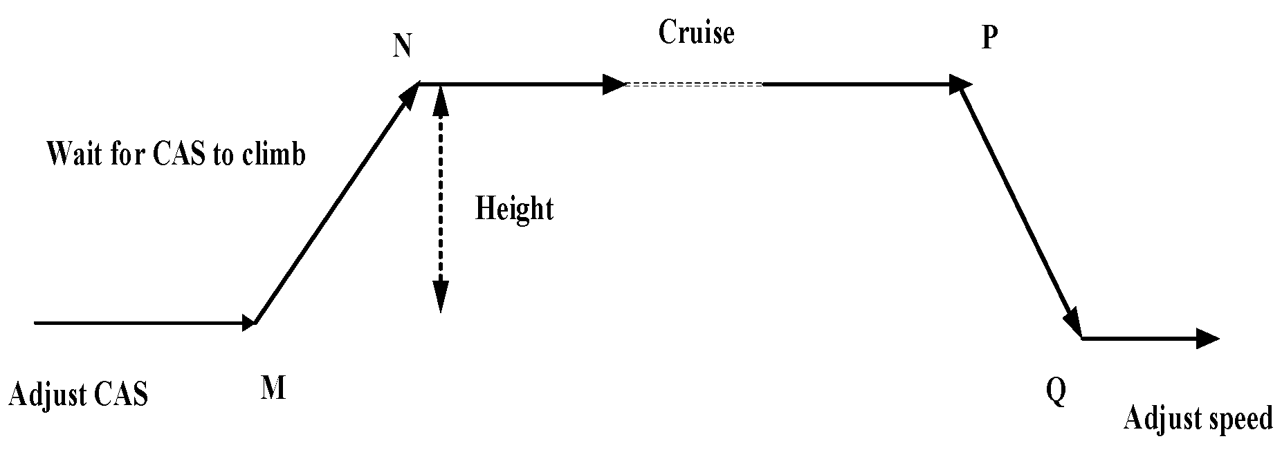
The basic aircraft profile in the flight path of civil aircraft is composed of equal speed level flight, equal calibrated airspeed climb (CAS), equal Mach climb, equal CAS descent, equal Mach descent, equal altitude deceleration, etc., as shown in Figure 1. In it, the cruise flight stage is the main flight mode and the main body of ad hoc network communication. Therefore, the influence of motion change on the communication network when the aircraft adjusts its altitude is ignored.

Figure 1.
Basic flight profile.
This is because the several other stages of the flight are very short in duration and soon switch to a horizontal mode of flight. The calculated value of the horizontal position of the aircraft in the ascending stage will be slightly ahead of the actual position of the aircraft, and the calculated value of the horizontal position of the aircraft in the descending stage will also be slightly ahead of the actual position of the aircraft. These problems need to be combined with the actual flight altitude, flight speed, transmission delay and other parameters in the actual flight to slightly correct the aircraft position.
- (2)
- Flight level track
From a typical horizontal flight path, it can be known that aircraft usually follow a straight line from one waypoint to another or near that point, turn and take a new course, and fly in a straight line again. Horizontal flight routes are all composed of linear flight segments and arc flight segments. The aircraft speed and direction remain unchanged in the linear flight segment, while inscribed turn is most commonly used in the arc flight segment (as shown in Figure 2). Vi and Vj in the figure are take-off and landing cities, P1 and P2 are waypoints, route segment ViP1 is the straight flight segment, and the route segment is the arc flight segment. The flight path of the straight section can be described as:
where is the coordinate position at time t, v is the velocity and is the direction of motion.
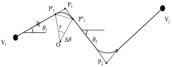
Figure 2.
Horizontal flight path diagram.
The turning problem of the arc flight segment can be described as follows: given the coordinates of the waypoints, the position of the initial point and the end point of the turn can be solved. As the coordinates of waypoints Vi, P1 and P2 in Figure 2 are known, the coordinate calculation process of the turning starting points P′1 and P″1 is as follows:
That is, the magnitude and direction of the turning angle can be expressed as:
In Formula (4):
Then, , that is: ; therefore, the coordinates of the starting point of the turn are:
In addition, the flight path or speed direction of the aircraft during the turning process can be considered as a uniform angle change. Therefore, the flight path of the arc segment can be described as:
where is the angle formed between the aircraft i and the center of the turning circle at moment t − 1, and is the variation of the turning angle per unit of time.
2.3. Aircraft Location Algorithm
In order to facilitate the research, the position of the aircraft during flight is located on the basis of the known aircraft flight path in this paper.
Through the implementation of Algorithm 1, it can accurately calculate the time when the aircraft reaches a certain point, and it can also know the position of the aircraft at any time, thereby completing the basic work before clustering.
| Algorithm 1 Aircraft location algorithm |
|
3. Clustering
In order to facilitate the research and analysis of the clustering algorithm of civil aircraft, let us make the following assumptions:
- (1)
- The perception radius of all aircraft nodes is equal to the propagation radius, that is, the communication radius;
- (2)
- The flight path of the aircraft is known and flown in strict accordance with the plan, that is, through Algorithm 1, the information such as the position coordinates of the aircraft can be calculated at any time.
The main difference between the clustering algorithm based on the known trajectory and the traditional algorithm is that the clustering deployment has been completed before the aircraft flight, and the aircraft needs to store the clustering information and identity information list related to its own routes and flights. After the aircraft takes off, according to the pre-planned clustering situation, the geographical location information is obtained by GPS and the identity identifier is changed accordingly (such as the identification of the cluster, the status in the cluster, whether it is a gateway, etc.) and the clustering work is automatically completed, thereby reducing the additional overhead such as forming clusters.
3.1. Division of Geographic Clusters
Definition 1.
Geographic cluster: cluster divided by geographic region.
The aircraft communication in the geographic cluster must be forwarded by the cluster head and the geographic inter-cluster relies on the gateway for communication, so the geographic cluster is a plane cluster structure.
Theorem 1.
A circle with a communication radius of R makes communication coverage for the area with its inner regular hexagon, and loophole-free coverage with minimal repetitive coverage can be obtained.
Proof.
If the angles of several congruent regular polygons are placed at a point, then they can satisfy the loop-free coverage, that is:
where is the inner angle of the regular n-polygon, and to ensure that x is a positive integer, the values of n are 3, 4 and 6. Let us assume that the area of the circle with communication radius R is Sc and the area of its inner regular n-polygon is Sp, then the repeated coverage area Sd of a node circle region after the loop-free coverage is:
It is easy to know from Equation (10) that when n = 6, the repeated coverage area is the smallest. Therefore, a circle with a communication radius of R can obtain loophole-free coverage with minimal repetitive coverage and the most ideal cluster structure by making communication coverage for the area with its inner regular hexagon. □
Through Algorithm 2, we can understand how to divide geographic clusters.
| Algorithm 2 Geographic cluster partitioning algorithm |
|

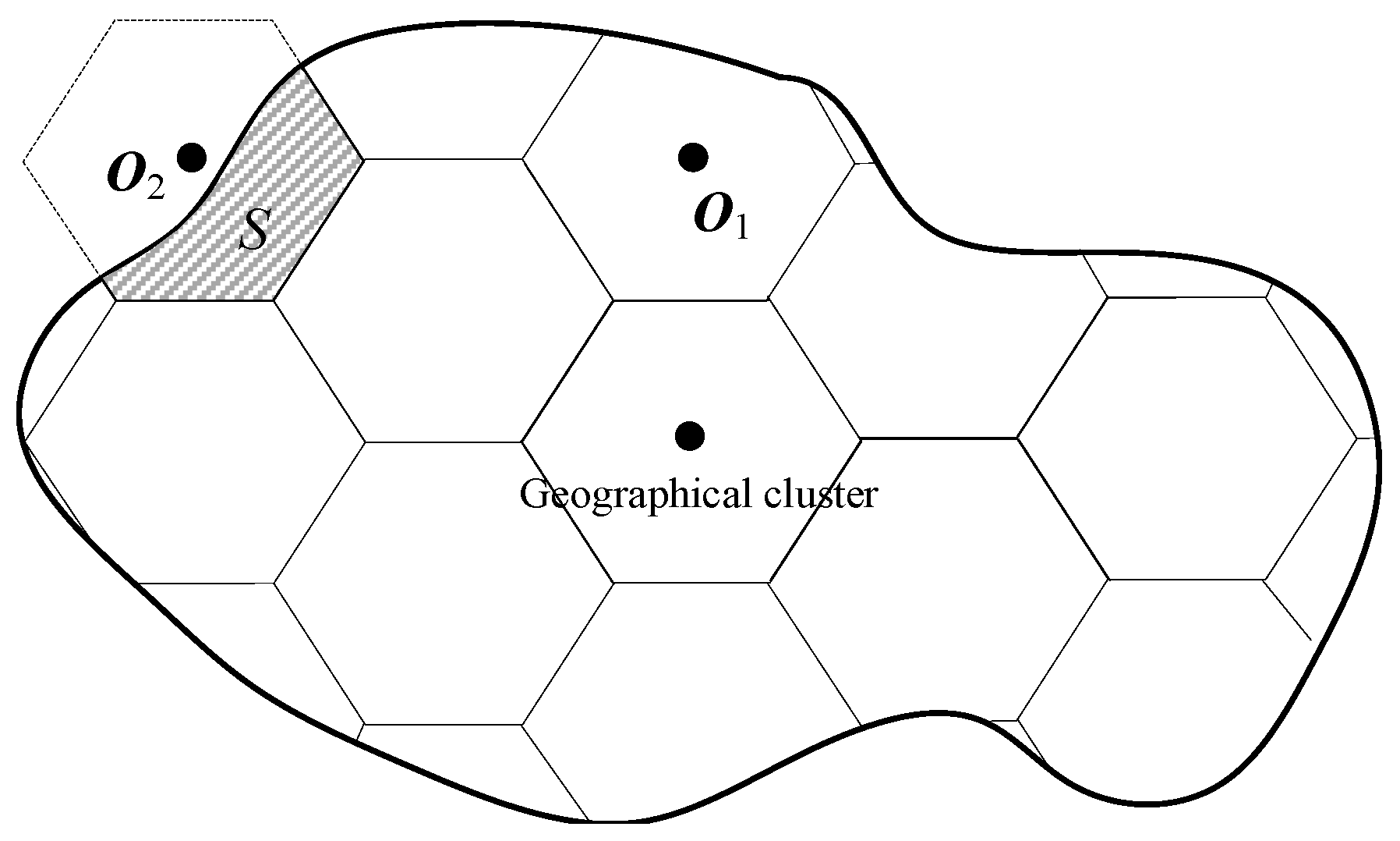
Figure 3.
Diagram of geographic cluster partitioning algorithm.
Figure 3.
Diagram of geographic cluster partitioning algorithm.
Theorem 2.
When dividing geographical clusters, if the center of a hexagon is outside the boundary of the aircraft region, ignoring the region will not affect the communication of the aircraft within it.
Proof.
Since the flight boundary is determined by the take-off and landing cities and route distribution, when the center of a hexagon is outside the boundary of the aircraft area (O2 in Figure 3), it means that there must be take-off and landing cities in the area S and the communication range of the airport can cover S. Therefore, ignoring the aircraft in this area, communication will not be affected by clustering. □
Theorem 3.
When an aircraft belongs to a geographic cluster, it can maintain communication with other cluster members in the cluster.
Proof.
Saivichit C. et al. [27] came to the conclusion that the distribution of aircraft on the route has the characteristics of Poisson distribution after analyzing the actual data. Suppose that aircraft A has just flown into a geographic cluster, then if there is another aircraft in the geographic cluster and the aircraft is within the communication range of A, it can be demonstrated that it can communicate with other cluster members in the cluster. □
Let us set the aircraft density be , then the probability of n aircraft in airspace D follows the Poisson distribution:
In Formula (11), SD is the area of airspace D, so the probability P that the aircraft can communicate with other cluster members is:
where SD meets the requirement of R = 300 km. According to statistics, between 8:00 and 24:00 every day, the density of aircraft is , then:
Therefore, the theorem holds.
According to Theorem 3, the communication between cluster heads and cluster members can be guaranteed by establishing geographic clusters in the above method through Algorithm 2.
3.2. Geographical Cluster Head Region Division
Definition 2.
Geographical cluster head region: in a geographical cluster, when an aircraft reaches a certain airspace in the cluster, it can become the cluster head if the corresponding conditions are met, and this area is called the geographical cluster head area.
Geographical cluster head region division method: take the center of the geographical cluster as the center of the circle, select the radius R/2 as the radius of the geographical cluster head region, and the circular region formed accordingly is the geographical cluster head region, as shown in Figure 4.
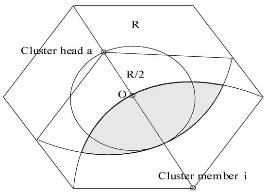
Figure 4.
Communication diagram between cluster head and cluster member 2.
Theorem 4.
Any plane in the geographic cluster will not reach the cluster head more than two hops.
Proof.
Take aircraft i, if there is an aircraft that can communicate with both aircraft i and the cluster head, it can be proven that any aircraft will not exceed two hops to the cluster head. Assuming that cluster head a just flew into the geographic cluster head region and became the cluster head, then the distance between any aircraft in the geographic cluster and a is no more than 3R/2. Let us place aircraft i furthest from the cluster head. If there is an aircraft in the shaded region as shown in Figure 4, then the aircraft can communicate with aircraft a and i simultaneously. □
It is easy to know from mathematical knowledge that , according to the proof process of Theorem 1; similarly, the probability P that there is an aircraft in this region is:
Therefore, any aircraft in the geographic cluster will not reach the cluster head more than two hops, which ensures the effectiveness of the cluster head communication coverage and avoids the situation of communication instability caused by excessive hops.
Definition 3.
Affiliated cluster member: a node that can communicate directly with the cluster member but cannot communicate directly with the cluster head due to the limited communication distance.
The affiliated cluster member has certain flexibility and can communicate with other nodes through the cluster member, thus avoiding the generation of isolated communication nodes. Because there are cluster members in the geographic cluster which are not within the range of one hop of the cluster head, in order to avoid the interruption of the connection with the cluster head, it can be forwarded by other cluster members within one hop. The setting of the affiliated cluster members increases the flexibility of the cluster and ensures the coverage of the geographic cluster on the nodes.
Definition 4.
Initial cluster head: the cluster head formed when a certain aircraft first flies to the geographical cluster head area.
The initial cluster head is usually the first aircraft of the route in a day, which is a prerequisite for the formation of the initial cluster, mainly satisfying the information forwarding within the initial cluster, and it is then replaced by a new cluster head.
3.3. Segmentation of Geographical Clusters
Due to the limited communication range of aircraft, the different geographical cluster heads cannot communicate directly, that is, the geographical clusters formed are plane clusters and the geographical clusters are connected through gateways. However, when the number of aircraft in a geographic cluster is too large, the burden of the cluster head and the overhead within the cluster will increase sharply. In order to reduce the overhead of cluster heads and reduce the message forwarding delay, geographical clusters need to be divided to form small clusters that are convenient for communication, and the heads of small clusters can communicate directly to form hierarchical structure clusters. Therefore, a cluster structure is formed with the whole network angle being a planar cluster and the local area angle being a hierarchical cluster.
Definition 5.
Geographic cluster threshold Nmax: when the number of cluster members of a geographic cluster exceeds a certain value, it needs to be divided into clusters, and this value is called the geographic cluster threshold.
The setting of a geographic cluster threshold reduces the communication burden of cluster heads, and avoids cluster head load aggravation or even communication blockage due to an excessive number of nodes in the cluster.
Definition 6.
Communication subcluster: a small cluster formed by segmentation of geographic clusters according to a certain algorithm (Algorithm 3) to facilitate communication.
| Algorithm 3 Generation algorithm of communication subclusters |
|
Definition 7.
Advanced cluster: a cluster with the geographic cluster head as the cluster head, and the communication subcluster head as the cluster member is formed in the geographic cluster head region.
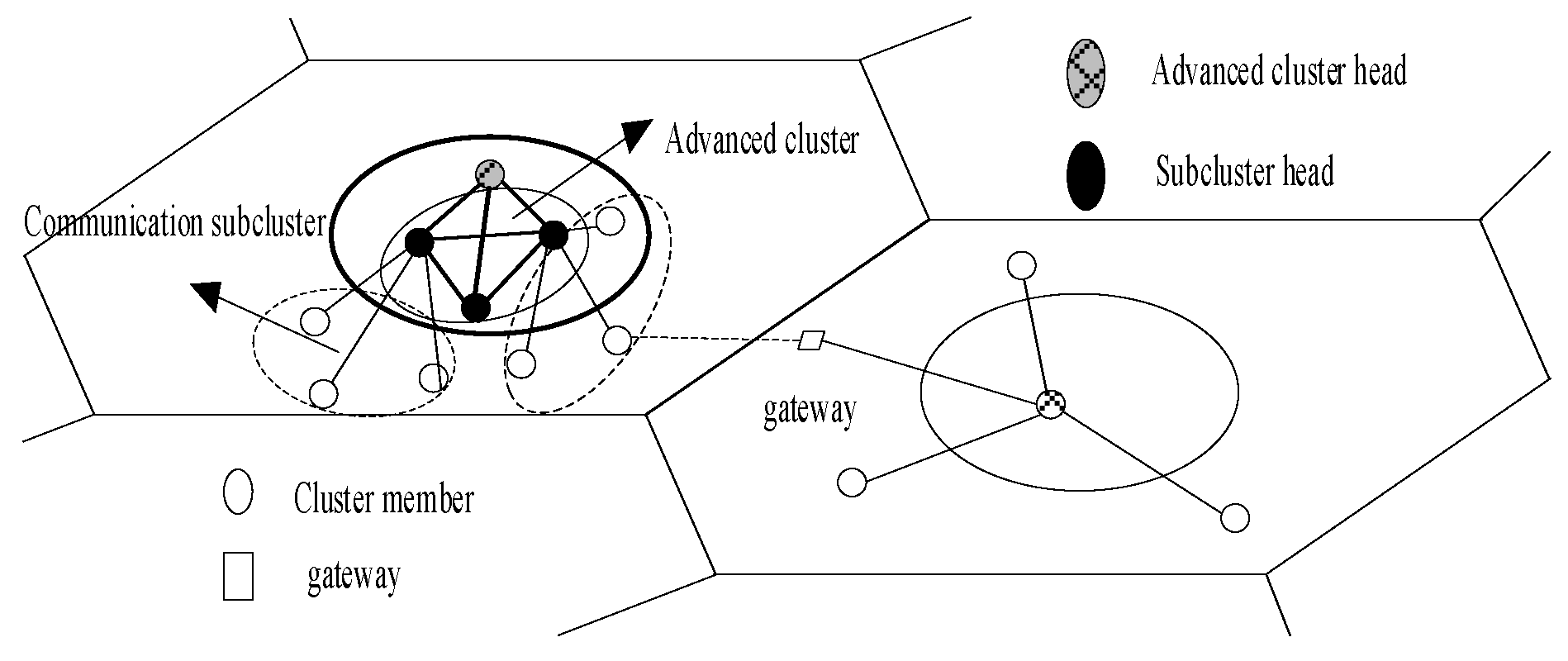
In order to control the scale of geographical clusters, if the number of cluster members in a cluster exceeds the threshold of geographical clusters, it is necessary to divide the communication subclusters. The original geographical cluster head acts as the head of the advanced cluster and the cluster head of the formed communication subcluster is the cluster member of the advanced cluster. The communication subclusters of the same geographic cluster communicate with each other through advanced clusters, while the communication between different geographic clusters is carried out through gateway nodes. Different from geographical clusters, in order to reduce the number of forwarding times, cluster members in advanced clusters can communicate directly with each other. The network structure is shown in Figure 5.
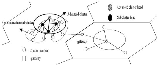
Figure 5.
Network topology.
Definition 8.
Cluster capacity Ncapacity: the number of cluster members when the cluster is in optimal state.
Theorem 5.
In an ideal state, for a network with n nodes, the optimal number of clusters is, and the number of cluster members in the cluster is also.
Proof.
According to Qi [28], the whole network can be divided into m clusters. In order to ensure the traffic balance of the whole network, the traffic bandwidth of the whole network B2 is equally distributed to each subnet, namely . The transmission traffic S of each node, the transmission traffic of a node within a subnet Ssubnet and the traffic of the cluster head node Sbackbone are, respectively, , , where B represents the channel bandwidth and is the coefficient factor. In the ideal case, , thereby obtaining the cluster number Since the total traffic of nodes in the subnet is the traffic of the cluster head of the subnet in the backbone network, ; therefore, , and thus, . □
If the total number of aircraft in the network at a certain time is n, assuming that all geographical clusters are hierarchical clusters, then it is known from Theorem 5 that the optimal number of clusters is and the cluster capacity is . In addition, according to Definition 5, when the number of cluster members exceeds the geographical cluster threshold, it is necessary to divide them. Since the number of communication subclusters divided is at least two, the geographical cluster threshold is set at . In practice, aircraft density is associated with geographical location, so the division of geographical clusters needs to combine the number of ideal clusters, cluster capacity, regional aircraft density and other factors. The generation algorithm of communication subclusters is as Algorithm 3.
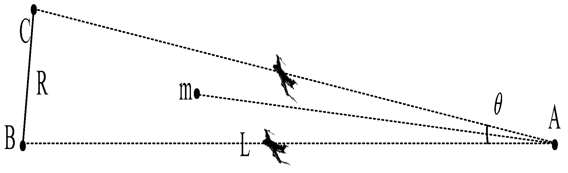
Among them, the number of communication subclusters in step 2 is . In step 4, the communication subclusters are divided according to the angle, that is, the aircraft with similar route angles are divided into a subcluster. This method maintains the stability of the formed subclusters. As shown in Figure 6, let the route angle formed by route AB and AC be . If two aircraft a and b take off from route AB and AC at point A at the same time, respectively, the conditions for them to maintain communication are as follows: the distance from aircraft a to b is not greater than the communication radius R. Therefore, the distance for which the two aircraft can maintain communication state while flying is: .

Figure 6.
Diagram of route AB and AC course angles.
Let R = 300 km and when , L = 1728 km. Therefore, when the route angle of the two routes is very small, the relative motion between the aircraft is very small, and the communication remains very stable. If the aircraft can communicate with each other at some time, the communication state will be maintained for a long time. Therefore, in this algorithm, nodes with similar route angles and small relative motion are divided into the same subcluster to reduce the amount of cluster recombination.
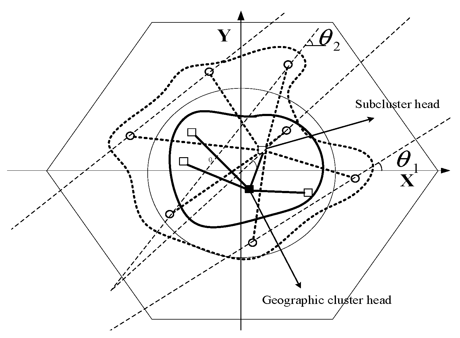
According to Step 5, it can be known that the aircraft in the geographic cluster head area and on the route closest to the geographic cluster center can serve as the subcluster head for a relatively long time, and the cluster head is convenient to form advanced clusters. In particular, the cluster members of the formed advanced clusters are all within the communication range of the cluster head, thus facilitating the formation of hierarchical structures. The communication subcluster structure diagram is shown in Figure 7.
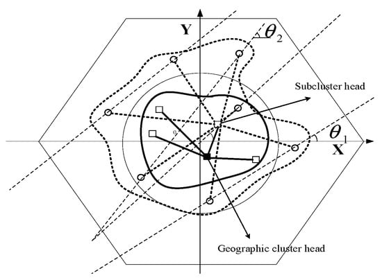
Figure 7.
Communication subcluster of . The outer dashed circles indicate geographic clusters, the inner thick solid circles indicate high-level clusters, and the middle thin circles indicate ideal communication subclusters.
3.4. Gateway Selection
The communication between geographical clusters cannot rely on the cluster heads to communicate with each other, so the concept of gateway needs to be introduced.
The gateway generation algorithm is relatively simple, that is, when an aircraft leaves the original geographic cluster and flies to a new geographic cluster, it can act as a gateway node because the aircraft maintains a communication relationship with the original geographic cluster and can also maintain communication with the new cluster. Only one gateway node needs to exist between two adjacent geographic clusters. When the original gateway node flies out of the communication range of the original geographic cluster member, the gateway identity is automatically cancelled and the new aircraft takes over. On the one hand, the existence of gateway can enhance the communication between geographical clusters and facilitate the formation of network topology. On the other hand, the turbulence of cluster structure is reduced. When an aircraft becomes a gateway, it still maintains a link connection with the original cluster member in a certain period of time, communication interruption caused by updating clusters is avoided and communication continuity is increased.
3.5. Clustering Algorithm Process
Algorithm 4 shows the clustering method we implement.
| Algorithm 4 Clustering algorithm |
|
4. Performance Analysis
4.1. The Formation of Clusters
- (1)
- Clustering overhead
Because this algorithm (Algorithm 4) uses the knowledge of the flight track to complete the clustering by predicting the position distribution of aircraft, the whole clustering process is completed before the aircraft takes off and the aircraft only needs to store the information related to itself. When the aircraft flies to the relevant position, the cluster identification is automatically changed and the communication is directly through the cluster structure. Therefore, no clustering overhead is required during the clustering process.
- (2)
- Intra-cluster maintenance overhead
The update of the maintenance stage of the cluster is still automatically completed by the aircraft according to its own position and combined with the flight time, so the cluster maintenance cost is also not required; especially when the number of aircraft is large, its advantage is more obvious. However, the aircraft increases the storage cost.
4.2. About the Cluster Itself
- (1)
- Number of cluster heads
Since this algorithm is based on geographic clusters, the clusters formed are planar structures from the perspective of the whole network, and the cluster scale is reasonably controlled by introducing the method of geographic cluster region, so that the number of clusters will be kept at a low level. From the perspective of geographical clusters, in order to prevent too many cluster members within a cluster, the threshold of geographical cluster is used as the standard for whether to divide communication subclusters and after dividing subclusters, and different channels are adopted for intra-cluster and inter-cluster, so as to ensure the stable work of the network after clustering and that the traffic between subclusters is balanced as far as possible. Through the above methods, the number of cluster heads and the scale of clusters can be maintained in the best state.
- (2)
- Cluster stability
Algorithm 4 adopts three ways to ensure the stability of the cluster:
- ➀
- From the perspective of cluster heads, the division of the geographic cluster head region makes the location of cluster heads have centrality in both the geographic cluster and the communication subcluster. In particular, the selection criteria of cluster head of communication subclusters are based on proximity to the geographic cluster center and survival time in the cluster head region, which also ensures the stability of cluster heads.
- ➁
- From the perspective of cluster members, the communication subcluster divides aircraft on the routes with similar flight angles into the same cluster, which avoids the existence of relatively large moving aircraft in the same subcluster, thus ensuring the stability of cluster members.
- ➂
- From the perspective of gateway, the establishment of gateway ensures the continuity of cluster communication and avoids network turbulence caused by aircraft leaving the original geographic cluster. At the same time, it can maintain contact with multiple cluster heads to be responsible for information forwarding and other works, thus completing the network structure of the cluster and increasing the stability of the cluster structure.
- (3)
- Load balancing
The load of a cluster head depends on the number of nodes it supports. Maintenance of cluster structure and inter-cluster routes all need to consume certain resources of cluster heads. Therefore, we do not want the situation of some cluster heads being overloaded and some cluster heads being idle to exist.
In Algorithm 4, load balancing is improved in three ways:
- ➀
- Due to the dynamic change in the geographical cluster head, aircraft can act as cluster heads as long as the conditions are met and the election of cluster heads is fairer. With a large geographical cluster coverage, the extreme situation of too many and too few aircraft in the geographic cluster will not occur, so the load balance of the geographical cluster head in the whole network is guaranteed.
- ➁
- When there are too many cluster members in the cluster head, in order to avoid excessive load, the partitioning algorithm of communication subclusters is used to achieve load balancing of the cluster head within the communication subclusters.
- ➂
- Through the cluster member, the information of the affiliated cluster member is forwarded, which reduces the communication burden of the cluster head and keeps a good load balance.
5. Simulation Verification
5.1. Experimental Environment
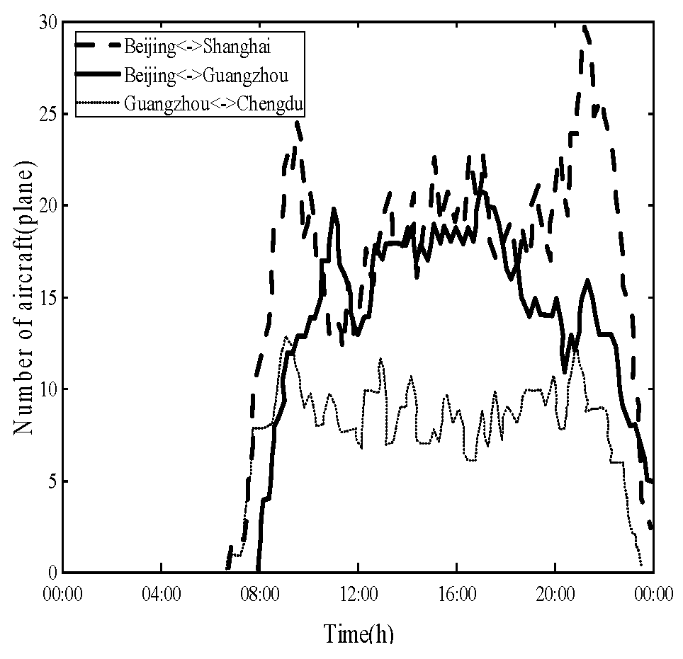
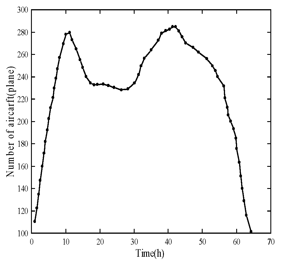
In order to verify the performance of the clustering algorithm in the actual environment, based on the flight information of the routes between Beijing, Shanghai, Guangzhou, Chengdu, Kunming and other important cities, the distribution and flight situation of the actual routes are constructed. According to the take-off and landing time, location and flight route of all flights throughout the day, the flight process is calculated using Matlab. The distribution of the city locations and some routes is shown in Figure 8. The number of aircraft on some important routes and the statistical results of the total number of aircraft on the above-mentioned routes are shown in Figure 9 and Figure 10.
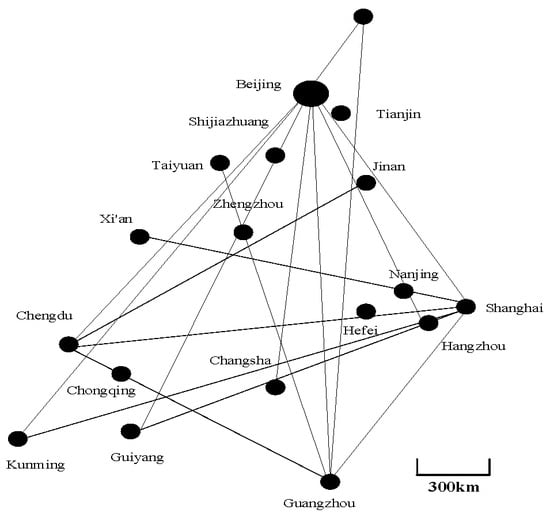
Figure 8.
City location and distribution of some routes.
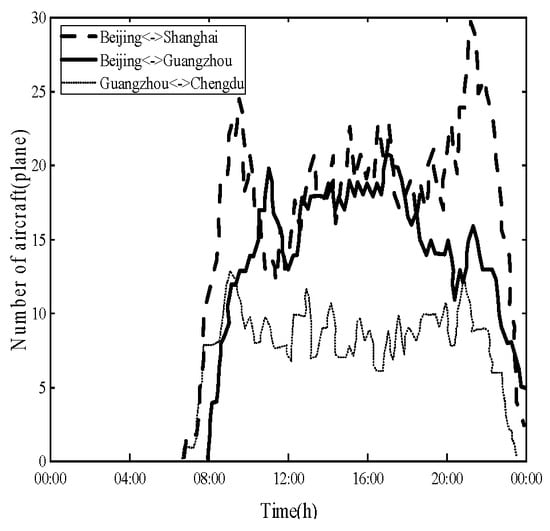
Figure 9.
Chart of the number of aircraft on some important routes changes over time.
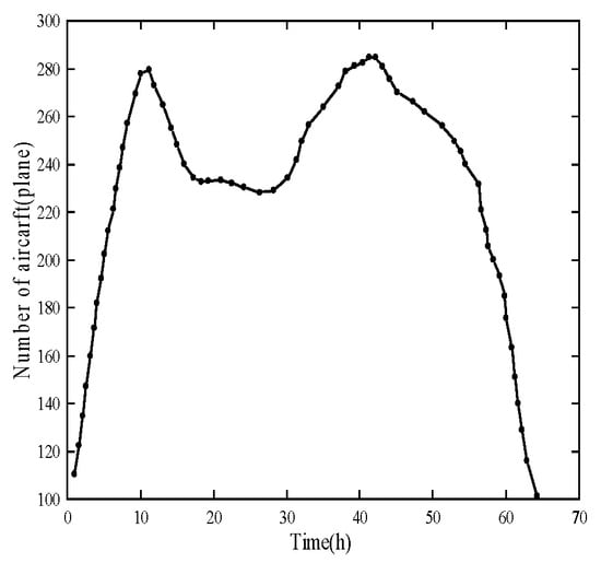
Figure 10.
Chart of the total number of aircraft on some routes changes over time.
It can be seen from Figure 9 and Figure 10, during 00:00 to 6:00, the number of flights on China’s main routes is small, while during 8:00 to 24:00, the number of planes on the routes is large, and the density of planes in the air is large and stable, which meets the conditions for the formation of aviation ad hoc network. Therefore, when comparing and verifying the clustering performance, the simulation is mainly carried out between 8:00 and 24:00. In this paper, the actual data such as the above-mentioned routes and flight distribution are used as the conditions and parameters of the clustering performance simulation experiment, and the experimental environment is built accordingly.
5.2. Performance Analysis
Since the Lowest-ID and Max-Degree are classical clustering algorithms, this paper will compare with them to verify the performance of the algorithm proposed in this paper.
- (1)
- Clustering structure
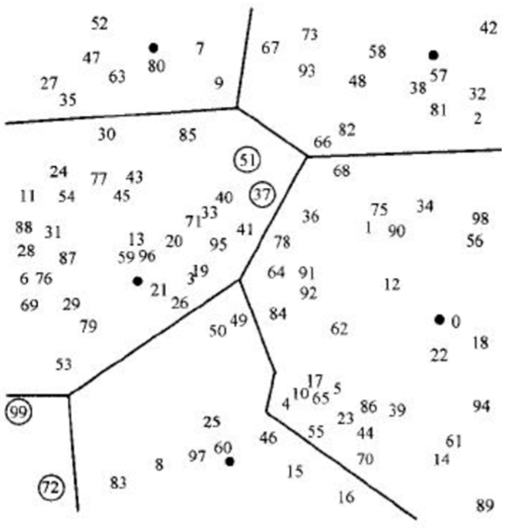
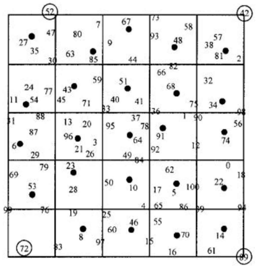
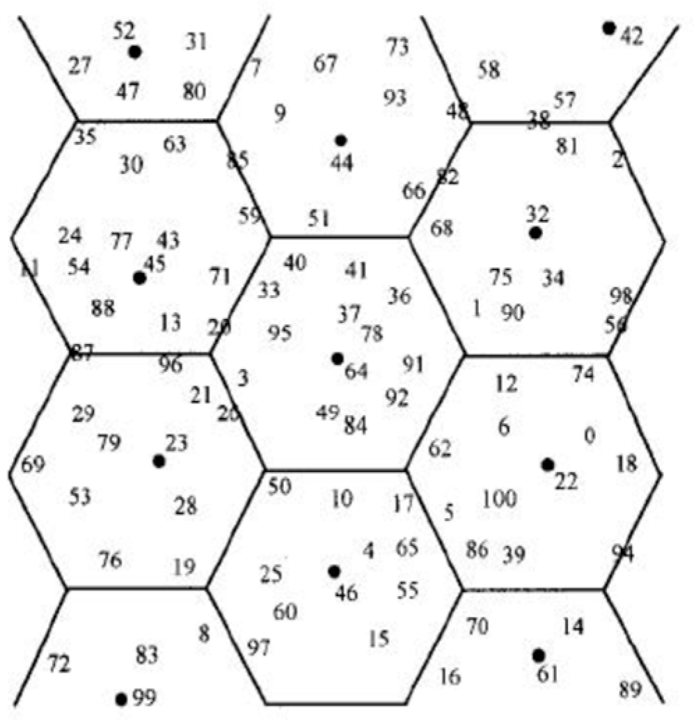
Figure 11, Figure 12 and Figure 13, respectively, show the clustering structures formed by the Lowest-ID algorithm, Max-Degree algorithm and the proposed method. Among them, the solid black dot represents the cluster head. It can be seen from the figures that in both Lowest-ID and Max-Degree algorithms, there are clusters composed of one or two nodes and the number of formed clusters is large, and the number of nodes in the clusters is not uniform.

Figure 11.
Clustering structure of Lowest-ID algorithm.

Figure 12.
Clustering structure of Max-Degree algorithm.

Figure 13.
Clustering structure of the proposed method.
- (2)
- Number of formed clusters
Test 1 The number of formed clusters from the perspective of the whole network
In order to compare the performance of the three algorithms in the number of formed clusters from the perspective of the whole network, according to the above experimental environment, the communication radius is set to 300 km and the statistical results of the number of formed clusters between 6:00 and 24:00 are shown in Figure 14.
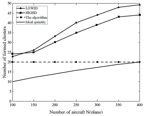
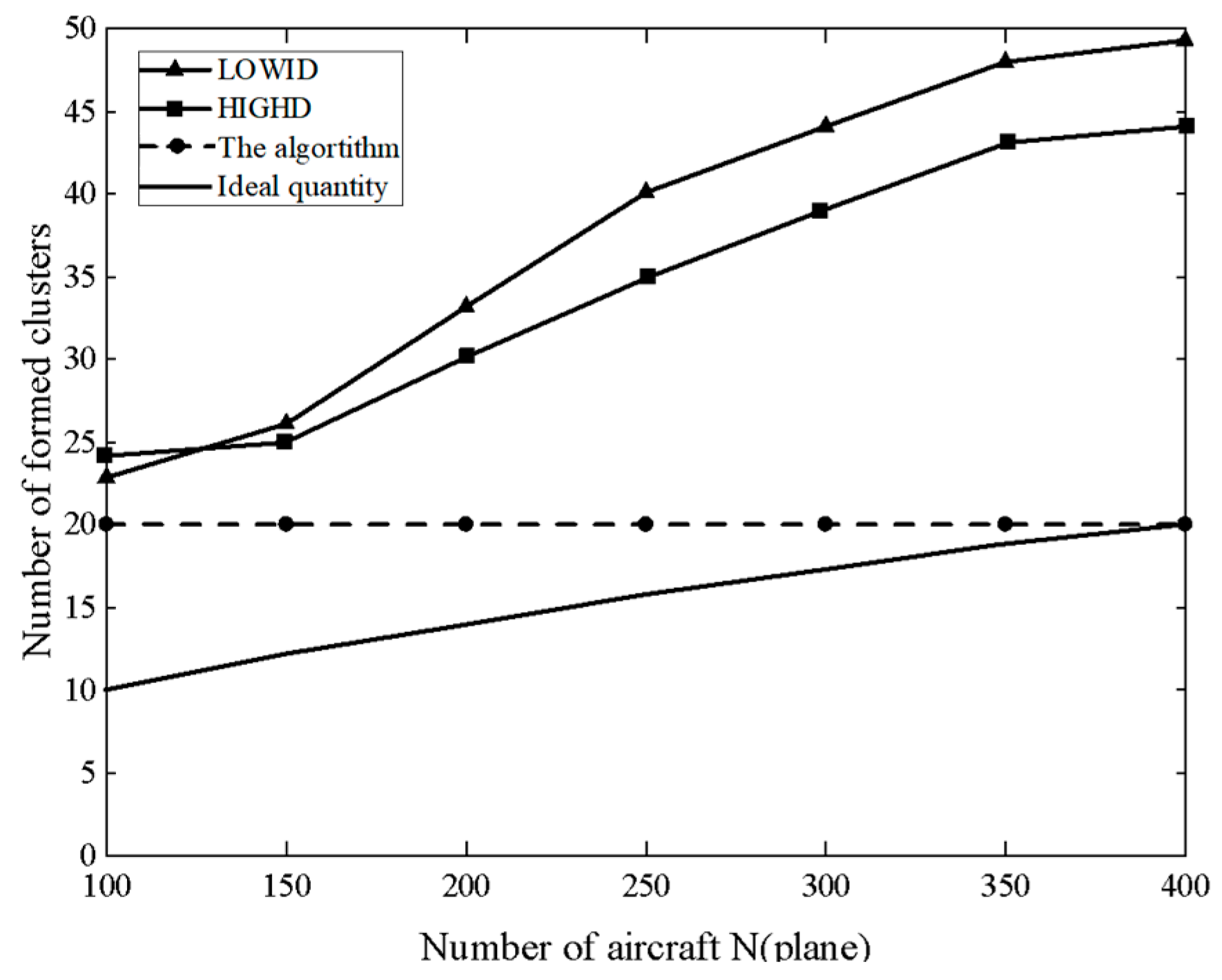
Figure 14.
Number of formed clusters from the perspective of whole network.
Test 1 Result analysis:
Since it is in a cluster of planar structure, for inter-cluster communication carried out through the gateway, the smaller the number of cluster heads, the smaller the number of hops between nodes and the better the performance of the network. It can be seen from Figure 14 that the number of clusters formed by this algorithm is the lowest and remains unchanged. This is because when the number of clusters is counted from the perspective of the whole network, the algorithm takes the geographical cluster as the unit, which has a large coverage area, so the number of formed clusters is minimum. In the other two algorithms, the number of formed clusters is affected by the number and density of aircraft in the network, so the volatility is high. In addition, combined with the cluster structure, it is easy to know that the number of clusters between any two aircraft in the whole network is no more than five, which effectively improves the route forwarding efficiency.
Test 2 The number of formed clusters from the angle of geographic cluster
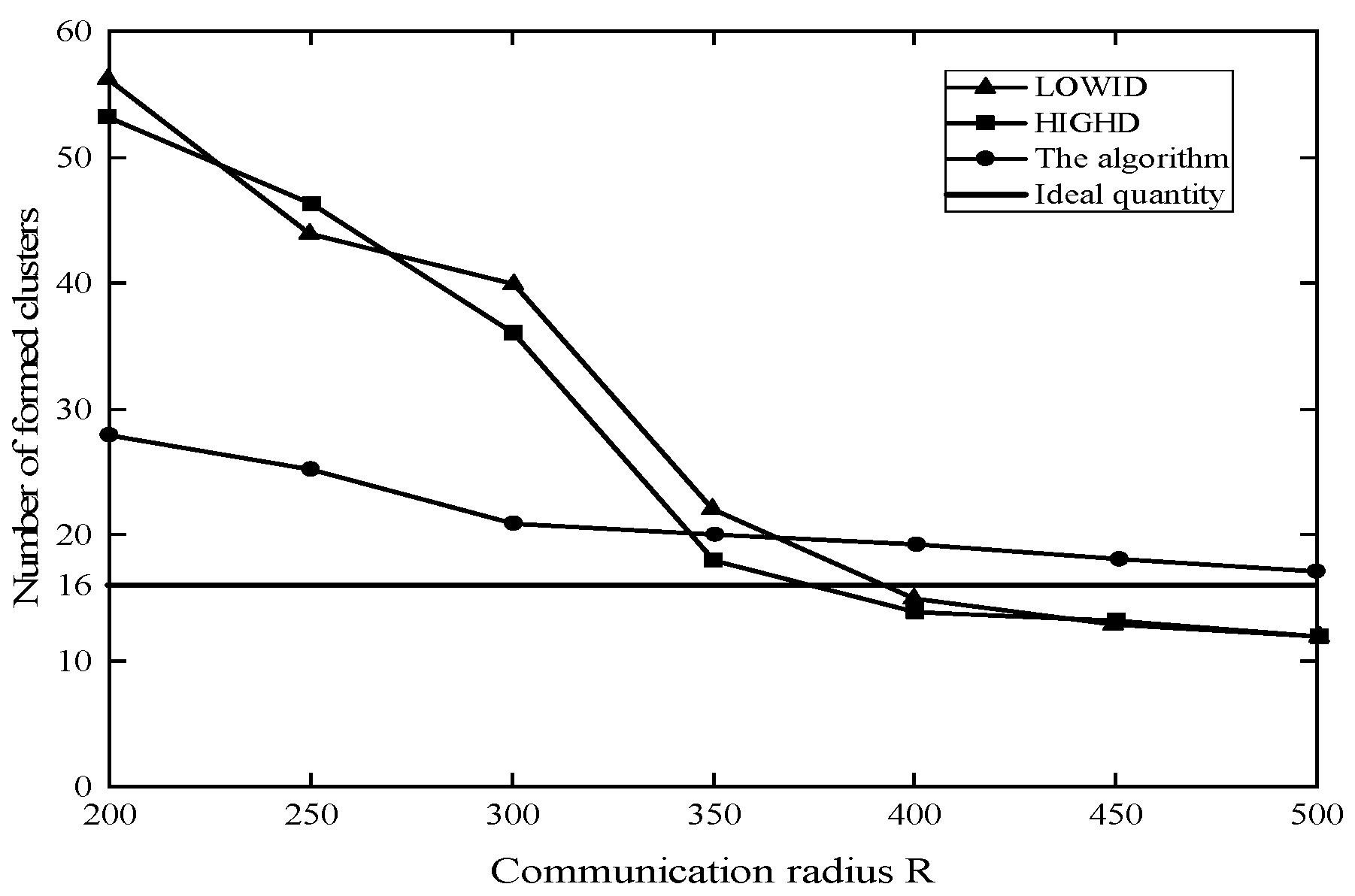
According to the analysis in Section 3.3, when the density of aircraft in a certain area is high, if the number of clusters is unreasonable, the burden of cluster heads will be too large and even the communication will be blocked. Therefore, the regular hexagonal region centered in Nanjing was selected as the research scope in this test and the statistical results of the number of formed clusters within it are shown in Figure 15.

Figure 15.
Number of formed clusters from the perspective of geographical cluster.
Test 2 Result analysis:
This algorithm is closest to the number of ideal formed clusters. When the density of aircraft is high, the minimum ID and maximum connectivity algorithms do not limit the number and scale of clusters, which results in a large cluster scale and a large burden on the cluster head. However, this algorithm calculates the number of formed ideal clusters, takes the ideal number as the standard in the clustering process and makes adjustments within the range of one cluster difference, so it is the closest to the ideal formed cluster number.
- (3)
- Cluster stability
Test 3 Cluster head change frequency
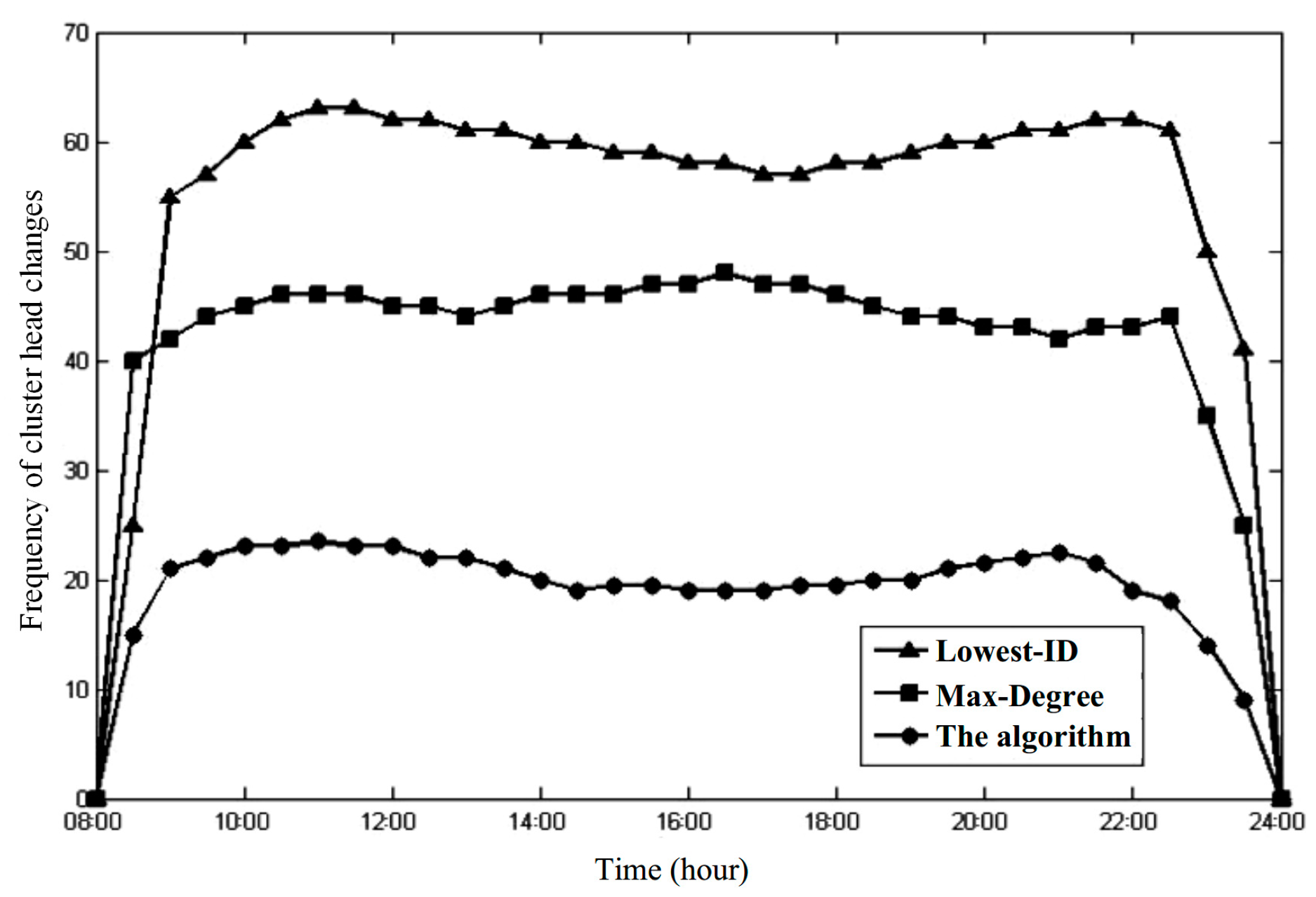
The change frequency of cluster heads is the number of cluster head changes per unit of time. The less the cluster node changes, the more stable the cluster structure is. The experiment was selected between 8:00 and 24:00, with 30 min as the unit time; the communication radius was 300 km and the experimental results of the cluster head change frequency are shown in Figure 16.
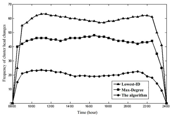
Figure 16.
Cluster head change frequency.
Test 3 Result analysis:
Under the same conditions, the number of cluster head changes in this algorithm is relatively lower. It can be seen from Figure 16 that the number of cluster head changes in the algorithm is slightly large between 8:00 and 8:30. This is because the initial cluster head first flies into the geographic cluster head region during this period and is not screened by the cluster head survival time, so its change frequency is slightly higher. In addition, during the peak flight periods of 9:00–11:00 and 18:00–20:00, the change frequency of cluster heads did not increase. The reason for this is that when the aircraft density is high, the survival time of the selected cluster heads in the geographical cluster head region will be longer; therefore, the change frequency of cluster heads will decrease.
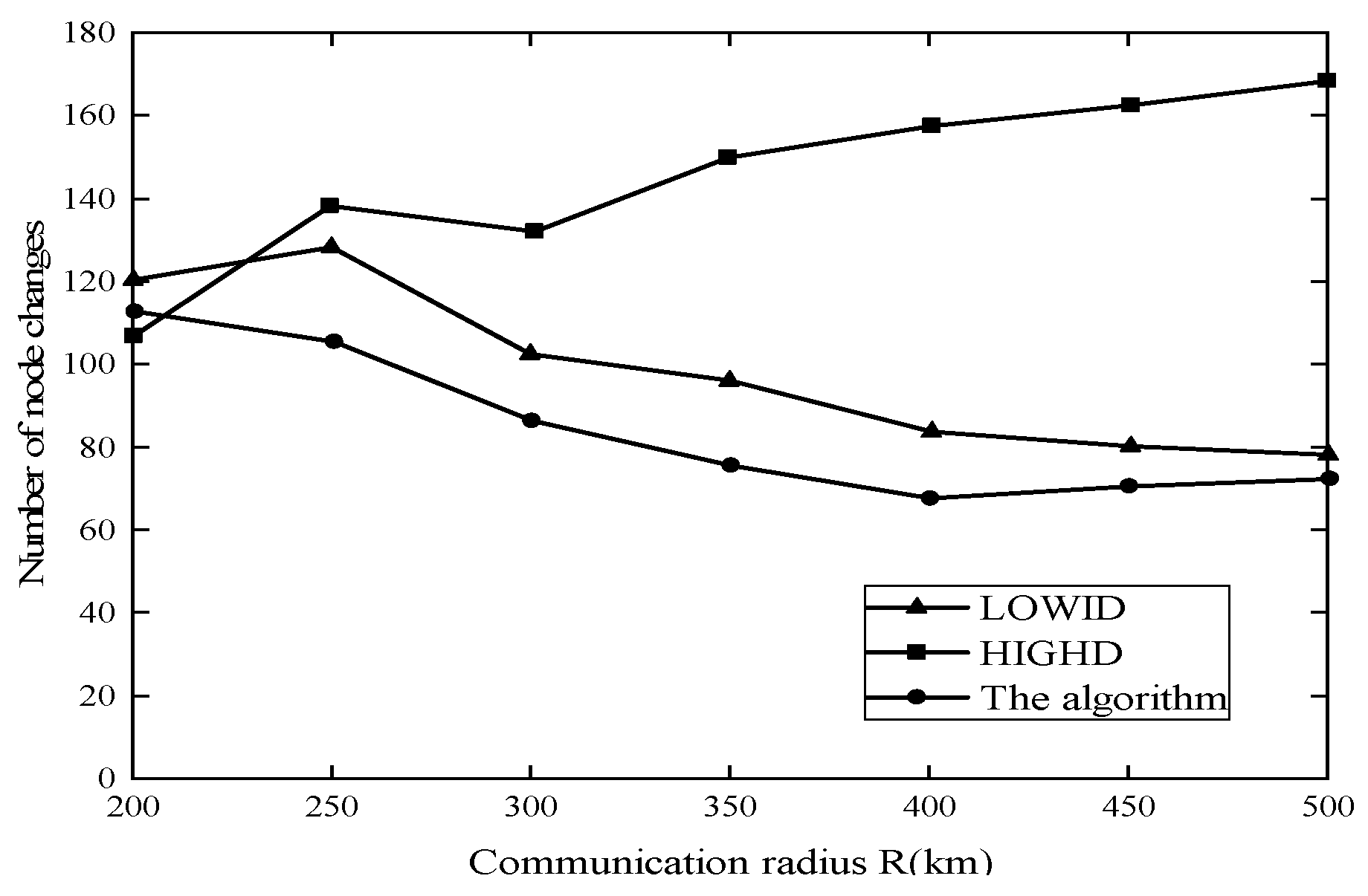
Test 4 Number of node changes
Aircraft nodes can serve as cluster heads, cluster members, gateways and other roles, while frequent changes in nodes can also reflect the instability of clusters. The experimental results of node changes per time unit are shown in Figure 17.
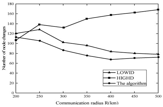
Figure 17.
Number of node changes.
Test 4 Result analysis:
During two peak flight periods, the node change frequency of the three algorithms all becomes higher, but under the same conditions, the node change number of this algorithm is relatively small. The reason for this is that when the number of nodes increases, the node change frequency of the three algorithms increases accordingly during the peak period. In the Lowest-ID and Max-Degree algorithms, when the cluster head changes, all nodes in the whole cluster have to change. However, when the cluster head changes in this algorithm, the geographical cluster does not change and the cluster members also belong to the original geographical cluster, thus greatly reducing the change frequency of cluster member nodes.
- (4)
- Load balancing of cluster heads
Because of the dynamic changes in the network, nodes often join or leave a cluster, so it is difficult to keep the system in a good load-balancing state. In order to measure the balance of cluster heads in communication, the following formula is adopted as the evaluation standard.
where xi is the number of cluster members in cluster head i, u is the number of average neighbor nodes in cluster head , N is the number of nodes in the network and nc is the number of cluster head nodes. A larger value indicates better load balancing.
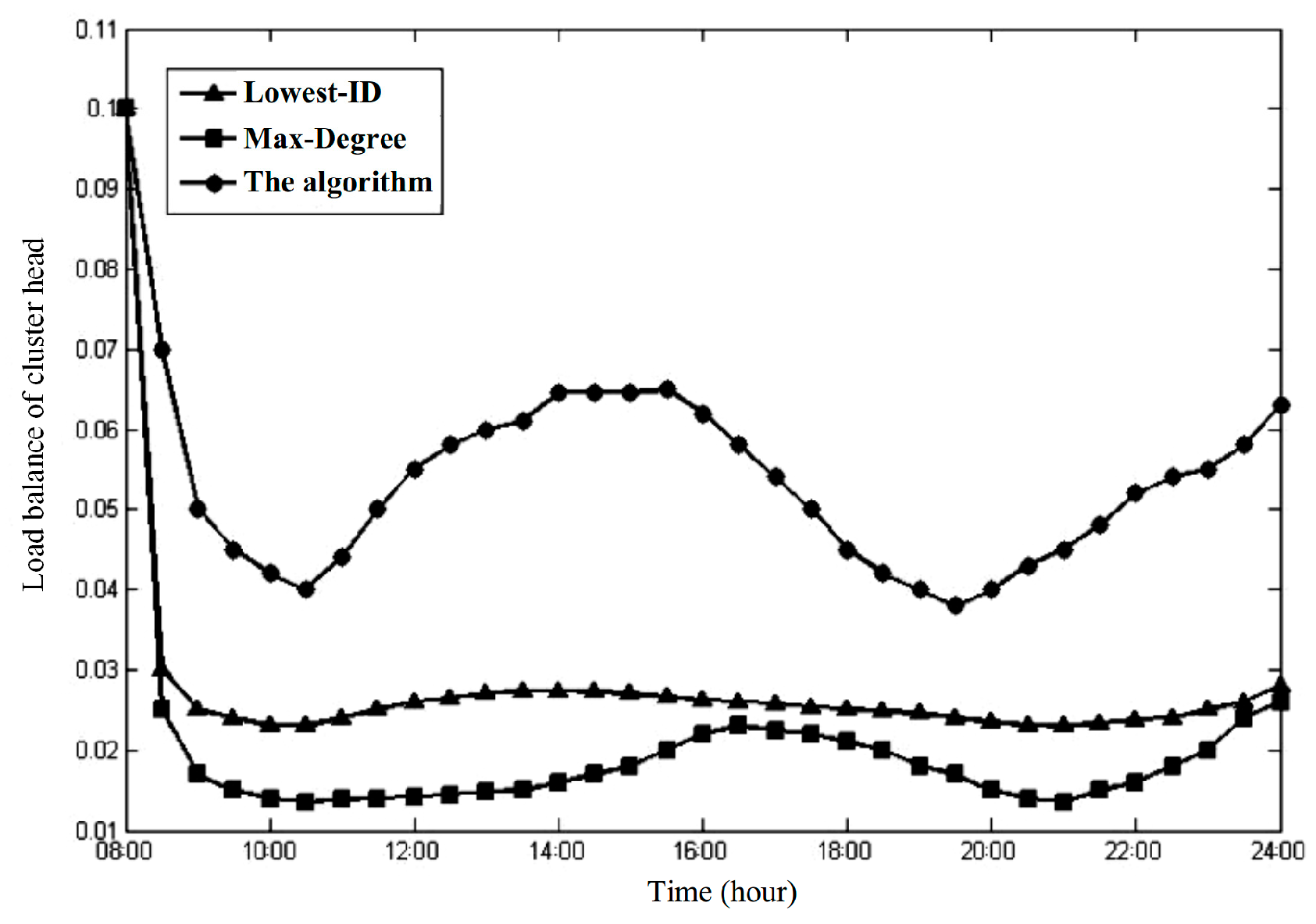
Test 5 Cluster head load balancing from the perspective of whole network
According to Equation (14), the load balancing of cluster heads was simulated and calculated from the perspective of the whole network and the experimental results are shown in Figure 18.
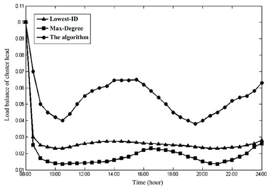
Figure 18.
Load balance of cluster head from the perspective of whole network.
Test 5 Result analysis:
Under the same conditions, the LBF value of this algorithm is the largest, that is, the balance of cluster heads is the best. This is because the geographical cluster covers a large area, the number of aircraft in it does not fluctuate greatly. In the Lowest-ID and Max-Degree algorithms, the number of cluster members in an individual cluster can reach tens at most, or only one or two at least. Therefore, the LBF value is the highest, and the load balance of cluster heads is also the worst.
6. Discussion
With the continuous development of civil aircraft communication technology, the ordinary aviation telecommunication network can no longer meet the increasing demand for communication. The establishment of aviation ad hoc network has become an important means of current aviation communication. Therefore, the clustering algorithm used for AANET has become a hot research topic. Moreover, at present, the number of flights in China is huge and increasing day by day. A superior clustering performance can efficiently solve the problems faced by the establishment of aviation ad hoc network (AANET) such as poor routing performance and limited network scale. In this paper, a new clustering algorithm, that is, a zero-overhead clustering algorithm for AANET based on known trajectory, is proposed in the context of the increasing importance of trajectory prediction to the current air transportation system. It is proposed on the basis of obtaining the relevant information of an aircraft’s flight position and route through modeling and accurately obtaining the aircraft’s position information at any time through the aircraft positioning algorithm. Before an aircraft takes off, geographical clusters and cluster head regions are divided by the geographical cluster division algorithm, and geographical clusters with too many aircraft in the cluster are divided by the communication subcluster generation algorithm. In this way, cluster information is stored to complete cluster deployment. Then, after the aircraft takes off, according to the relevant cluster information stored before takeoff, combined with the geographical location information obtained by GPS, the cluster head, gateway node and other identifiers are updated by themselves, so as to automatically complete the work of forming clusters and updating and maintaining them. Finally, the proposed clustering algorithm is verified using the actual route data. Compared with the traditional minimum ID clustering and maximum connectivity methods, the proposed algorithm has a great improvement in the structure and stability of clusters, the number of clusters and the load balance of the cluster head. Figure 11, Figure 12 and Figure 13 are the schematic diagrams of the clustering structures of the three algorithms. By comparison, it can be seen that the number of clusters formed by this algorithm is small and the number of nodes in the clusters is uniform and its clustering structure is stable. Figure 14 and Figure 15 discuss the number of clusters from the perspective of the whole network and geographical clusters. It can be seen from Figure 14 that this algorithm has the smallest number of clusters, while Figure 15 shows that this algorithm is closest to the ideal number of clusters. Since the lower the number of cluster heads, the better the network performance and the more the number of clusters deviates from the ideal value, the more the cluster heads are likely to be overburdened or the communication is blocked, it can be seen that the number of clusters in this algorithm is better. Figure 16 and Figure 17 discuss the cluster stability from the perspective of cluster head change frequency and node change frequency. It can be seen from Figure 16 that the cluster head change frequency of this algorithm is the lowest and it can be seen from Figure 17 that the node change frequency of this algorithm is the lowest. The fewer the number of changes of cluster heads and nodes, the more stable the cluster structure. This shows that the cluster stability of this algorithm is better. Figure 18 explore the load balancing of cluster heads in terms of network-wide and geographic clusters. It can be seen from Figure 18 that the LBF value of this algorithm is the largest in both cases, that is, the equilibrium of cluster heads is the best.
The cluster formation overhead and cluster maintenance overhead of the aviation ad hoc network (AANET) clustering algorithm determine the resource utilization of the civil aircraft during communication. The algorithm proposed in this paper is automatic in both the cluster clustering work and the cluster maintenance work. In the cluster formation stage, the aircraft position is predicted by utilizing the known trajectory to complete the clustering and information storage before takeoff. The aircraft automatically changes the cluster identification after flying to the relevant position, and communicates directly through the cluster structure, thus the cluster formation overhead is zero. In the maintenance stage, the aircraft automatically completes the updating and maintenance of the clusters according to its own position and flight time, thus the cluster maintenance overhead is zero. This point is not involved in the clustering algorithm proposed before. For example, although Pathak [29,30] designed new clustering algorithms from the perspective of reducing the frequency of cluster head changes and cluster formation overhead, the results could not achieve the intended goal of zero overhead in the cluster formation and other processes. Li, CHEN, LIN, YU [31,32,33,34] also improved the old clustering algorithm based on the node location information, their experimental results also showed obvious performance gains in the network lifetime, energy efficiency, energy consumption balance and other performances, but they also could not achieve energy zero overhead in the cluster formation process. Zang [35] designed a mobility prediction clustering algorithm for high-speed environments, which is based on the principle of using GPS to provide node location and movement information to build node movement prediction models, thus solving the problem of high mobility when aircraft are used as mobile nodes. However, when the nodes are highly mobile, the cluster head and cluster structure will change rapidly, leading to a large maintenance overhead; although this algorithm improves on this, there is still a certain amount of energy waste.
The superior clustering performance of the proposed method can solve the problems such as poor routing performance and limited network scale faced by the establishment of aviation ad hoc network (AANET), thus improving the stability and performance of the network. Moreover, the advantage of zero overhead can avoid the unnecessary waste of resources caused by civil aviation aircraft in communication, thus saving energy. This method has potential application value to communication between civil aircraft. However, whether the increased cluster storage overhead is too large when the number of aircraft is large and how to ensure that the time complexity of the clustering algorithm is low remains to be studied in the future.
7. Conclusions
Combined with the characteristics of civil aviation ad hoc network, a zero-overhead clustering algorithm based on known track is designed in this paper. Firstly, by establishing the route model and track model, the aircraft location algorithm is used to obtain the geographical position coordinates of the aircraft at any time. Then, on this basis, the geographic cluster partitioning algorithm and communication subcluster generation algorithm are used to complete the clustering work in advance. Then, the communication retention time of aircraft is considered comprehensively to complete the cluster update, the affiliated cluster member is used to avoid the generation of isolated communication nodes and the gateway node is utilized to maintain the continuity of cluster communication, thus forming a network structure and increasing the robustness of clusters; then, the performance of the algorithm is analyzed theoretically. Finally, the performance of the algorithm is simulated using the actual route data. The experiment and analysis results show that the clustering cost and cluster maintenance cost of the algorithm are zero. In addition, compared with the traditional algorithm, this algorithm maintains a reasonable number of formed clusters, reduces the frequency of cluster head replacement, reduces the number of cluster members in and out of the cluster, avoids the loss of control of cluster heads to cluster members and effectively improves the overall stability of the cluster. How to ensure the security of the clustering process and how to design routing based on clustering are the focus of future research.
Author Contributions
C.L. and D.L.; writing—original draft preparation, L.L., P.L. and M.S.K.; writing—review and editing. All authors have read and agreed to the published version of the manuscript.
Funding
The work was funded by the Key Science and Technology Program of Henan Province (No. 222102210224, 232102211003, 232102210017), the Joint Fund Project of Science and Technology R&D Plan of Henan Province (No. 222103810044).
Data Availability Statement
The data used to support this research article are available from the corresponding author upon reasonable request.
Conflicts of Interest
The authors declare no conflicts of interest.
References
- Gurumekala, T.; Gandhi, S.I. A Cross Layered Routing Approach for Civil AANET. Wirel. Pers. Commun. 2022, 125, 619–635. [Google Scholar] [CrossRef]
- Bilen, T.; Canberk, B. Q-Learning Driven Routing for Aeronautical Ad-Hoc Networks. Pervasive Mob. Comput. 2022, 87, 19. [Google Scholar] [CrossRef]
- Gurumekala, T.; Gandhi, S.I. Toward in-flight Wi-Fi: A neuro-fuzzy based routing approach for Civil Aeronautical Ad hoc Network. Soft Comput. 2022, 26, 7401–7422. [Google Scholar] [CrossRef]
- Luo, C.-Y.; Song, Y.-L.; Gao, Z.-Z. Connectivity on fixed air route in aeronautical ad hoc networks. Tongxin Xuebao/J. Commun. 2014, 35, 147–155. [Google Scholar] [CrossRef]
- Yang, J.; Sun, K.X.; He, H.S.; Jiang, X.F.; Chen, S.W. Dynamic Virtual Topology Aided Networking and Routing for Aeronautical Ad-Hoc Networks. Ieee Trans. Commun. 2022, 70, 4702–4716. [Google Scholar] [CrossRef]
- Xu, J.; Xu, B.; Zhang, X.; Sun, Z. Improved minimum weighted clustering algorithm in wireless sensor networks. J. Nanjing Univ. Posts Telecommun. (Nat. Sci. Ed.) 2016, 36, 56–63. [Google Scholar] [CrossRef]
- Cheng, M.; Zhang, W.-Y.; MA, X.-S. The degree adaptive clustering algorithm based on maximum link degree clustering. J. Hefei Univ. Technol. 2010, 33, 60–63. [Google Scholar]
- Vatambeti, R.; Sanshi, S.; Krishna, D.P. An efficient clustering approach for optimized path selection and route maintenance in mobile ad hoc networks. J. Ambient. Intell. Humaniz. Comput. 2023, 14, 305–319. [Google Scholar] [CrossRef]
- Bilen, T.; Aydemir, P.J.; Konu, A.E.; Canberk, B.; IEEE. Customized K-Means Based Topology Clustering for Aeronautical Ad-hoc Networks. In Proceedings of the IEEE 26th International Workshop on Computer Aided Modeling and Design of Communication Links and Networks (CAMAD), Electr Network, Porto, Portugal, 25–27 October 2021. [Google Scholar]
- Shahbazi, M.; Simsek, M.; Kantarci, B. AI-enabled cluster head selection through modified density based clustering in Aeronautical Ad Hoc Networks. Ad. Hoc Netw. 2023, 148, 12. [Google Scholar] [CrossRef]
- Wang, Z.S.; Ding, H.W.; Li, B.; Bao, L.Y.; Yang, Z.J. An Energy Efficient Routing Protocol Based on Improved Artificial Bee Colony Algorithm for Wireless Sensor Networks. IEEE Access 2020, 8, 133577–133596. [Google Scholar] [CrossRef]
- Chang, L.Y.; Li, F.; Niu, X.Z.; Zhu, J.H. On an improved clustering algorithm based on node density for WSN routing protocol. Clust. Comput. J. Netw. Softw. Tools Appl. 2022, 25, 3005–3017. [Google Scholar] [CrossRef]
- Ahmad, M.; Hameed, A.; Ullah, F.; Wahid, I.; Rehman, S.U.; Khattak, H.A. A bio-inspired clustering in mobile adhoc networks for internet of things based on honey bee and genetic algorithm. J. Ambient. Intell. Humaniz. Comput. 2020, 11, 4347–4361. [Google Scholar] [CrossRef]
- Zhang, J.X.; Yan, R.Q. Multi-objective Distributed Clustering Algorithm in Wireless Sensor Networks Using the Analytic Hierarchy Process. In Proceedings of the 20th IEEE/ACIS International Conference on Software Engineering, Artificial Intelligence, Networking and Parallel/Distributed Computing (SNPD 2019), Toyama, Jamaica, 8–11 July 2019; pp. 88–93. [Google Scholar]
- Ergenç, D.; Eksert, L.; Onur, E. Dependability-based clustering in mobile ad-hoc networks. Ad. Hoc Netw. 2019, 93, 25. [Google Scholar] [CrossRef]
- Zhou, J.Y.; He, P.F.; Liu, Y.L.; Wu, W.G. Stable Clustering Algorithm for Routing Establishment in Vehicular Ad-Hoc Networks. In Proceedings of the 19th International Conference on Algorithms and Architectures for Parallel Processing (ICA3PP), Melbourne, Australia, 9–11 December 2019; pp. 107–115. [Google Scholar]
- Zhou, J.L.; Zhang, H.H.; Lyu, W.Y.; Wan, J.Q.; Zhang, J.P.; Song, W.K. Hybrid 4-Dimensional Trajectory Prediction Model, Based on the Reconstruction of Prediction Time Span for Aircraft en Route. Sustainability 2022, 14, 3862. [Google Scholar] [CrossRef]
- Griner, P.; SteinhOfler, R.; Leitgeb, E.; Flühr, H.; IEEE. Air Traffic Simulation and Modeling. In Proceedings of the 4th International Conference on Broadband Communications for Next Generation Networks and Multimedia Applications (CoBCom), Graz Univ Technol, Fac Elect Engn, Graz, Austria, 12–14 July 2022. [Google Scholar]
- Ma, L.; Tian, S. A Hybrid CNN-LSTM Model for Aircraft 4D Trajectory Prediction. IEEE Access 2020, 8, 134668–134680. [Google Scholar] [CrossRef]
- Xu, Z.F.; Zeng, W.L.; Chu, X.; Cao, P.W. Multi-Aircraft Trajectory Collaborative Prediction Based on Social Long Short-Term Memory Network. Aerospace 2021, 8, 115. [Google Scholar] [CrossRef]
- Zeng, W.L.; Quan, Z.B.; Zhao, Z.Y.; Xie, C.; Lu, X.B. A Deep Learning Approach for Aircraft Trajectory Prediction in Terminal Airspace. IEEE Access 2020, 8, 151250–151266. [Google Scholar] [CrossRef]
- Wu, Y.; Yu, H.Y.; Du, J.P.; Liu, B.; Yu, W.T. An Aircraft Trajectory Prediction Method Based on Trajectory Clustering and a Spatiotemporal Feature Network. Electronics 2022, 11, 3453. [Google Scholar] [CrossRef]
- Xie, L.; Wei, Z.L.; Ding, D.L.; Zhang, Z.R.; Tang, A.D. Long and Short Term Maneuver Trajectory Prediction of UCAV Based on Deep Learning. IEEE Access 2021, 9, 32321–32340. [Google Scholar] [CrossRef]
- Tran, P.N.; Nguyen, H.Q.V.; Pham, D.T.; Alam, S. Aircraft Trajectory Prediction With Enriched Intent Using Encoder-Decoder Architecture. IEEE Access 2022, 10, 17881–17896. [Google Scholar] [CrossRef]
- Zhang, Z.Z.; Wei, Z.L.; Nie, B.W.; Li, Y. Discontinuous maneuver trajectory prediction based on HOA-GRU method for the UAVs. Electron. Res. Arch. 2022, 30, 3111–3129. [Google Scholar] [CrossRef]
- Choi, H.C.; Deng, C.H.; Hwang, I. Hybrid Machine Learning and Estimation-Based Flight Trajectory Prediction in Terminal Airspace. IEEE Access 2021, 9, 151186–151197. [Google Scholar] [CrossRef]
- Thi, X.M.N.; Miyanaga, Y.; Saivichit, C. Connectivity Modeling Analysis in Flight-Path Based Aviation Ad Hoc Networks. IEICE Trans. Commun. 2011, E94B, 1606–1616. [Google Scholar] [CrossRef]
- Qi, Q.; Wang, K.; Du, Y. Clustering Scheme Based on Spectrum Sensing in Cognitive Radio Ad hoc Networks. J. Data Acquis. Process. 2018, 33, 41–50. [Google Scholar] [CrossRef]
- Pathak, S.; Jain, S. A priority-based weighted clustering algorithm for mobile ad hoc network. Int. J. Commun. Netw. Distrib. Syst. 2019, 22, 313–328. [Google Scholar] [CrossRef]
- Pathak, S.; Jain, S. Comparative study of clustering algorithms for MANETs. J. Stat. Manag. Syst. 2019, 22, 653–664. [Google Scholar] [CrossRef]
- Li, X.; Men, C.-G. A Cluster Algorithm Based Geographical Location Information for Wireless Sensor Networks. In Proceedings of the TEIN 2012—2012 3rd International Conference on Telecommunication and Information, Sanya, China, 8–10 August 2021; p. 6. [Google Scholar]
- Chen, X.; Luo, X.; Yang, J. Improved Clustering Routing Algorithm Based on Node Location and Residual Energy. Microprocessors 2022, 43, 13–17. [Google Scholar] [CrossRef]
- LIN, Q.; ZHANG, D.; WANG, C.; XU, K. Dual-cluster-head routing algorithm based on location information. J. Comput. Appl. 2015, 35, 606–609+632. [Google Scholar] [CrossRef]
- YU, N.; ZHOU, P. Clustering algorithm with known node location information. Sci. Technol. Inf. 2014, 12, 192–193. [Google Scholar] [CrossRef]
- Zang, C.H.; Zang, S.H. Mobility Prediction Clustering Algorithm for UAV Networking. In Proceedings of the IEEE GLOBECOM Workshops (GC Wkshps), Houston, TX, USA, 5–9 December 2011; pp. 1158–1161. [Google Scholar]


Disclaimer/Publisher’s Note: The statements, opinions and data contained in all publications are solely those of the individual author(s) and contributor(s) and not of MDPI and/or the editor(s). MDPI and/or the editor(s) disclaim responsibility for any injury to people or property resulting from any ideas, methods, instructions or products referred to in the content. |
© 2024 by the authors. Licensee MDPI, Basel, Switzerland. This article is an open access article distributed under the terms and conditions of the Creative Commons Attribution (CC BY) license (https://creativecommons.org/licenses/by/4.0/).