Abstract
China’s widely adopted expressway ETC system provides a feasible foundation for realizing co-operative vehicle–infrastructure integration, and the accuracy of ETC data, which forms the basis of this scheme, will directly affect the safety of driving. Therefore, this study focuses on the abnormal data in an expressway ETC system. This study combines road network topology data and capture data to mine the abnormal patterns of ETC data, and it designs an abnormal identification model for expressway transaction data based on TL-XGBoost. This model categorizes expressway ETC abnormal data into four distinct classes: missing detections, opposite lane detection, duplicated detection and reverse trajectory detection. ETC transaction data from a southeastern Chinese province were used for experimentation. The results validate the model’s effectiveness, achieving an accuracy of 98.14%, a precision of 97.59%, a recall of 95.44%, and an F1-score of 96.49%. Furthermore, this study conducts an analysis and offers insights into the potential causes of anomalies in expressway ETC data.
1. Introduction
Autonomous driving technology has been rapidly advancing, yielding mature results in research related to intelligent vehicles, including vehicle trajectory tracking [1], automatic obstacle avoidance [2], and more. These advancements are primarily based on vehicle sensors and environment-aware data [1,3]. Despite these developments, there are opportunities to enhance safety and efficiency. These improvements are necessary due to the inherent limitations in a single vehicle’s perception range and the lack of comprehensive understanding regarding road conditions ahead and behind. Transitioning from individual vehicle intelligence to connected-vehicle intelligence holds paramount importance for the advancement of autonomous driving and intelligent transportation systems [4]. The construction of smart expressways with cooperative vehicle–infrastructure coordination capability is emerging as a significant trend, and scholars have begun to carry out research on related technologies [3,4,5,6,7]. The C-V2X-based vehicle–road cooperative system and intelligent vehicle equipped with the necessary technology are currently undergoing trial testing in pilot areas [4,7]. Nevertheless, extensive deployment would necessitate substantial time, financial resources, and dedicated operational teams. However, China’s expressway ETC system is now widely used with more than 227 million accumulated ETC users and nearly one billion ETC transaction big data generated every day [8]. The well-established infrastructure and the vast data reservoir generated by the ETC system present significant advantages for the development of an ETC-based vehicle–road cooperative system. In recent years, researchers worldwide have conducted numerous studies related to smart expressways utilizing ETC data, including speed prediction [9], service area residence time estimation [10], exit–entrance toll station or service area flow estimation [11], and the design of expressway ETC simulation platforms [8].
During the actual operation of the ETC system, abnormal data are inevitably generated due to the influence of factors such as ETC system equipment failures and large vehicle shading [12]. The studies related to smart expressways based on ETC data have inevitably encountered abnormal data, and they are usually dealt with by direct deletion [9,11] with limited dedicated research on ETC abnormal data. However, as ETC data are an important support of the vehicle–road cooperative system, the correctness of ETC data will directly affect the safety of driving. Conducting research on abnormal data within the ETC dataset is beneficial for troubleshooting issues and enhancing overall data quality. Therefore, this paper will carry out research on the detection of abnormal data in expressway ETC data. The analysis of anomaly data in expressway ETC big data encounters the following challenges.
In order to solve the above problems, this study defines the correct travel trajectory, classifies and analyzes the abnormal data, and then proposes an expressway transaction data abnormality identification model for identifying the abnormal patterns in the ETC big data of Chinese expressways. This study lays the foundation for the proper handling of abnormal data in intelligent expressway research based on ETC big data. It also offers valuable insights for practical operation and management, carrying significant research and practical significance.
The main contributions of this study are as follows:
- This study presents an efficient and precise multi-classification recognition model designed to identify specific anomaly patterns within the extensive expressway ETC dataset.
- We establish accurate vehicle trajectories derived from expressway ETC data to delineate our study’s focus. Subsequently, we categorize expressway ETC abnormal data into four distinct classes, aiming to enhance processing strategies tailored for different scenarios and ultimately improve overall data quality.
- This study validates the efficacy of the proposed method through lateral verification using captured data. Comparative analysis against baseline models demonstrates optimal performance across various evaluation metrics outlined in this paper.
The rest of this study is organized as follows. In Section 2, we review the research related to outlier detection and expressway ETC data anomalies. In Section 3, we introduce the data and its preprocessing process and describe the research problem. In Section 4, we describe the expressway transaction data anomaly identification method. In Section 5, we conduct experiments and analyze the results. Finally, in Section 6, we give the conclusions of this study and provide an outlook for future research.
2. Related Work
Anomaly detection is the problem of finding patterns in data that do not fit the expected behavior [13]. An outlier is a data point that is significantly different from other data points, or does not conform to expected normal behavior, or conforms well to defined abnormal behavior [14]. Current methods for anomaly detection include statistical-based anomaly detection [15], clustering-based anomaly detection [16,17,18], classification-based anomaly detection [19], integrated learning-based anomaly detection [20,21], etc.
Jay F. K. Au Yeung et al. [22] considered anomaly detection as a class imbalance problem by labeling classes for each timestamp and applying supervised learning models to learn the features of the labeled data, and then machine learning models are used for anomaly pattern recognition for jump detection in time-series data, which has good accuracy. Ya Su et al. [23] roposed the use of supervised learning models to study the patterns of normal data in multivariate time series to recognize anomalies, and the method has good robustness for various devices.
Jinbo Li et al. [24] proposed a clustering method to detect anomalies regarding the amplitude and shape of multivariate time series. However, it is essential to note that this method is tailored for continuous time-series data and may not directly address discrete data anomalies. Yassine Himeur et al. [25] proposed two anomaly detection algorithms for the detection of anomalies of electricity use in buildings. These include an unsupervised approach employing a single-class support vector machine, referred to as UAD-OCSVM, and a supervised method based on micro-moments, known as SAD-M2. Empirical evaluations revealed that SAD-M2 outperforms in terms of anomaly detection performance, real-time processing capabilities, and computational efficiency.
Elena Quatrini et al. [13] presented an industrial process anomaly detection method based on a two-step machine learning classification algorithm. The first step involves identifying the running process, and the second step focuses on anomaly detection. The anomaly detection process utilizes labeled data and the random forest algorithm. Hansi Chen et al. [26] introduced a framework for the anomaly detection of time-series SCADA data and the identification of critical equipment-monitoring parameters. Their approach is based on a Long Short-Term Memory Network–Auto-Encoder (LSTM–AE) neural network tailored specifically for anomaly detection in wind turbine status. Hao Xu et al. [27] introduced a data-driven anomaly detection algorithm for network intrusion. Their integrated approach incorporates oversampling and undersampling techniques to tackle the common dataset imbalance problem in anomaly detection. However, it is important to note that this method is primarily capable of detecting existing anomalies and may not adapt to newly emerging attack types resulting from technological advancements.
Vincent Vercruyssen et al. [28] presented a semi-supervised anomaly detection method aimed at automatically identifying anomalous behavior in time-series data. The primary objective is to enhance the efficiency and cost effectiveness of the production process. The method uses constrained k-mean clustering to perform initial unsupervised scoring and iteratively updates the anomaly scores by incorporating expert markers. Yu-Lin Tsou et al. [29] employed an optimally weighted single-class random forest approach for anomaly detection. They achieved this by constructing local random forests and forests using neighboring devices with the weights learned to minimize uncertainty in anomaly detection.
Juan Wang et al. [30] conducted a study employing edge computing and deep learning to analyze highway video surveillance data, achieving intelligent anomaly detection within highway surveillance networks. Xiliang Wang et al. [31] investigated abnormal driving vehicles and explored the relationship between highway vehicle braking, deflection, and deviation states with traffic accidents. They employed an improved grey correlation analysis method to discuss various scenarios, driver states, and violations, determining their associated risk probabilities. Muhammad Zubair et al. [32] analyzed the risk probabilities across different scenarios, driver states, and violations. Their study focused on real-time highway anomaly detection using image processing algorithms, significantly improving model recognition performance and speed. This advancement aids in timely accident detection, rescue operations, and congestion relief. Yue Hu et al. [33] conducted research on highway driving behavior detection, utilizing the recursive graphical attention network. Their study significantly enhanced the model’s recognition performance in identifying highway driving behavior anomalies, thereby advancing individual vehicle anomaly recognition capabilities.
Anomaly pattern analysis based on expressway ETC data-related studies in the literature follows. Qiqin Cai et al. [10] investigated vehicle entry into service area identification and residence length estimation using ETC data. Their classification of anomalous data involves removing redundant records, rectifying trajectories with context from the ETC gantry network topology, and omitting trajectories with incomplete data. Despite its comprehensive pre-processing, the approach has limitations. Fumin Zou [9] and others, in their study of speed prediction based on expressway ETC data, found that anomalous data existed in the dataset and deleted the anomalous data directly. However, none of these studies in the literature have an accurate classification of expressway ETC data anomalies, and there is no set of efficient and accurate fast identification methods. In this paper, based on the analysis and research of expressway ETC data, new types of anomalies are found, some of the anomaly types of expressway ETC data are labeled, and the anomaly detection is converted into a supervised multi-classification problem to improve the accuracy and efficiency of detection.
3. Preliminary
3.1. Data Source
The experimental dataset used in this study comprises three components. The first part consists of transaction data extracted from the toll system of an expressway located in a province in China. The second component comprises data captured by gantry devices positioned along the same expressway in that province. The third part encompasses data related to the topology of the gantries within the toll system on the expressway in the same province. Notably, the gantry capture devices and the toll system roadside unit devices are arranged in pairs on the gantries. In an ideal scenario, the records in these two datasets should correspond to each other. The gantry topology data record the placement of gantries along the expressway. In the following sections, we provide a detailed description of each of these three dataset components.
Transaction data from the expressway toll system include transaction data from gantries, entrance toll stations and exit toll stations, Table 1, Table 2 and Table 3 show the main fields of these data, respectively. The provincial expressway toll system can amass over 5 million transaction records daily, involving approximately 500,000 vehicles each day. These vehicles encompass four types of passenger cars, six types of trucks and special operations vehicles. The transaction data contain the desensitized itinerary number, gantry trading time, license plate number, type of vehicle being charged, and transaction error code in addition to the number, name, and type of the transaction gantry. The ETC entrance toll station data contain the desensitized trip number and entrance transaction time in addition to the number and name of the entrance toll station. Similarly, the ETC exit toll station data contain the desensitized trip number and exit transaction time in addition to the number and name of the exit toll station. The data recorded by the gantry capture device are also tabular data. The main fields of the data recorded by the gantry capture device are shown in Table 4. It contains the license plate number, capture time, gantry number, gantry name, gantry type, capture type, etc. after desensitization. To facilitate the subsequent discussion, the vehicle trajectories and passing road segments generated from the ETC transaction data are defined as follows:

Table 1.
Description of partial fields in ETC flag transaction data.
Table 2.
Description of partial fields in ETC entrance toll station data.
Table 3.
Description of partial fields in ETC exit toll station data.
Table 4.
Description of partial cap record.
: A sequence of ETC transaction records arranged in chronological order to construct the ETC transaction gantry trajectory is referred to as the travel trajectory, denoted as TrajPath, and it is represented as follows:
where the transaction node typically represents the travel’s origin point, and the transaction node typically denotes the trip’s destination.
: A passage section is a sequential combination of two neighboring gantry transaction nodes within the vehicle’s TNodePath. It represents the section information generated by the interaction behavior between the vehicle and the ETC gantry and can be expressed as follows:
where and are the TNodes that are sequentially adjacent in the TNodePath, and they are referred to as the sector origin gantry and the sector destination gantry, respectively.
The gantry topology data can show the basic information of the gantries and their connectivity in the province, with each set of origin gantries and destination gantries adjacent and connected. The main fields of the gantry topology data are shown in Table 5.
Table 5.
Description of partial topo.
3.2. Preliminary
3.2.1. Data Cleaning
Data preprocessing is an important step in data mining and analysis. It serves to eliminate invalid or irrelevant data, reduce noise interference, precisely delineate the research scope, and enhance the accuracy and efficiency of pattern recognition. This section will introduce the method and process of data preprocessing for ETC transaction data and capture data.
First, we need to clarify the research object and remove redundant data. Specifically, the following two types of data need to be deleted:
- Marked error data in ETC data
ETC transaction data comprise the record generated when vehicles pass through a gantry, involving transactions between onboard units equipment and roadside unit equipment. Due to reasons such as equipment malfunctions and network transmission anomalies, it is inevitable that transaction data will contain some erroneous entries. The ETC system can identify certain exceptional data and assign an errcode value of 1 to the corresponding entries. These data fall under errors that the current ETC system can automatically exclude, and they should be removed from research involving intelligent transportation systems based on ETC data. Analyzing the data with an errcode of 1 has neither practical significance nor scientific research value. Therefore, these errors do not fall within the scope of this study and are directly removed.
- 2.
- Special vehicle data
Unlike ordinary vehicles such as passenger cars and trucks, special vehicles such as police cars, armed police cars, and emergency vehicles often have exceptions allowing them to travel without strictly adhering to traffic rules due to their work-related needs. Therefore, the travel patterns of these special vehicles are distinct. For this study, we exclusively focus on the transaction data of regular vehicles and do not analyze the transaction data of special vehicles.
3.2.2. ETC Transaction Data Integration and Conversion
We followed these steps for data integration and conversion. First, we integrated ETC transaction data, entrance toll station data, and exit toll station data, resulting in an integrated dataset with the seven fields detailed in Table 6. Then, the integrated dataset was grouped by passid and sorted by transaction time. Each ‘passid’ corresponds to a trip. Sorting the group by transaction time allowed us to generate the trip’s track chain table. The nodes of this chain table are structured, and the information they contain is outlined in Table 7. An example of a trip trajectory is illustrated in Table 8. In the final step, the trip trajectory chain table was restructured into chain tables that represent section trajectories. Each section trajectory chain table comprises only two nodes, symbolizing the start gantry and the end gantry. For a trip trajectory of length n, it can be divided into n-1 section trajectory chain tables. The trip trajectory depicted in Table 7 is reconstructed, resulting in the section trajectory chain table shown in Table 8. This is described in Algorithm 1.
Table 6.
ETC transaction fusion data.
Table 7.
Example of ETC vehicle trajectory.
Table 8.
Example of ETC trajectory section.
Figure 1 illustrates the travel trajectory and sector trajectory of vehicle V as it enters from the provincial boundary entrance gantry A, passes sequentially through gantry B, gantry C, gantry D, and then exits from the provincial boundary exit gantry E. The travel trajectory is represented as shown below:
| Algorithm 1: ETC Data and Toll Station Data Fusion and Trajectory Generation |
| Input: ETC Transaction Table; Entrance Toll Station Table; Exit Toll Station Table; Output: ETC Trajectory
|
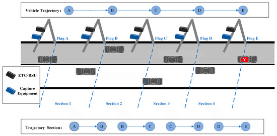
Figure 1.
Schematic diagram of section trajectory (example trajectory and example section trajectory are derived from ETC system data when vehicle V passes through the gray direction section).
3.2.3. Anomaly Pattern Mining Based on ETC Trajectory and Captured Trajectory
Capture data are utilized for reference in the analysis of ETC data. Expressway capture record data are exclusively recorded as vehicles traverse road sections without any records at entrance or exit toll stations. Furthermore, the capture data lack a ‘passid’ field, meaning there is no unique identifier to segment travel tracks. To create comprehensive travel tracks and segment them, the captured data must be integrated with entrance and exit toll station data. Upon comparing captured data trajectories with ETC trajectories, four distinct types of abnormal ETC data were identified: missing detections, opposite lane detection, duplicated detection and reverse trajectory detection. Algorithm 2 describes the capture data processing process. Algorithm 3 is Anomaly Pattern Mining Algorithm for Expressway ETC Data.
| Algorithm 2: Capture Data and Toll Station Data Fusion and Trajectory Generation |
| Input: Capture Data; Entrance Toll Station Table; Exit Toll Station Table; Output: Capture Trajectory
|
| Algorithm 3: Anomaly Pattern Mining Algorithm for Expressway ETC Data |
| Input: ETC Trajectory; Capture Trajectory; topo # Select trajectories with the same passid Output: Abnormal Pattern Classification Statistics
|
3.3. Definitions
The expressway network employs the ETC gantry as a pivotal node that is capable of gathering passage information from all regions and vehicle trips. This study conducts an analysis of anomalous patterns in ETC data, primarily utilizing ETC vehicle travel trajectories. To facilitate subsequent discussion and differentiation, we first establish a definition for the correct travel trajectory.
Correct Travel Trajectory : A correct travel trajectory refers to a travel trajectory that thoroughly, accurately, and succinctly represents the vehicle’s journey on the expressway. The correct travel trajectory can be expressed as follows:
The correct travel trajectory is based on the definition of a travel trajectory TrajPath and must satisfy the following conditions simultaneously:
- The transaction node is either the entrance toll station or the provincial boundary gantry, and the transaction node is either the exit toll station or the provincial boundary gantry;
- There are no repeated transaction nodes within the travel trajectory. In other words, are all distinct;
- Each preceding transaction node is connected to a subsequent transaction node. For instance, there is a connection between any transaction node from to ;
- The Dijkstra path length between adjacent transaction nodes is exactly 2.
The schematic diagram of the correct travel trajectory is depicted in Figure 2. This diagram illustrates the unique route taken by each trip along with the corresponding times when the vehicle passes through each gantry, allowing for an accurate reconstruction of the travel path.
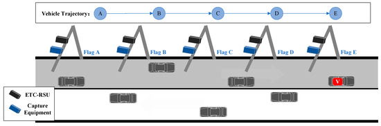
Figure 2.
Schematic diagram of the correct travel trajectory.
An abnormal travel trajectory is defined as any trajectory that does not align with the criteria for a typical travel trajectory. In such cases, there is at least one abnormal gantry pair within an abnormal travel trajectory that exhibits at least one type of abnormal pattern. After thorough investigation, it has been determined that ETC transaction data anomalies predominantly feature the following four types of patterns:
- (1)
- Reverse Trajectory
A reverse trajectory occurs when the sequence of gantries represented in the trip trajectory contradicts the trajectory data provided in the topology dataset. The schematic diagram of the correct travel trajectory is depicted in Figure 3. For example, consider a travel trajectory that passes through three gantries in the order of gantry A, gantry C, and gantry B. Upon conducting a connectivity check using the topology data, it is revealed that gantry A to gantry C is not directly connected, and gantry C to gantry B is either not connected or not directly connected. This situation may arise due to a system error that records the time of passing through gantry B and gantry C as the same, resulting in a potential reversal in the order of gantry B and gantry C within the travel trajectory.
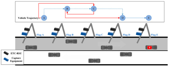
Figure 3.
Schematic diagram of reverse trajectory pattern.
The reverse recording rate is defined as follows:
where denotes the total number of reverse records and denotes the total number of section tracks.
- (2)
- Missing Detection
Missing detection refers to the occurrence of missing data when the gantry equipment fails to recognize a vehicle as it passes through the gantry. Potential causes of missing detection include weather changes, wireless crosstalk, equipment malfunction, and attempts at toll evasion. During a single trip, one or more missing detections may occur. These missing detections can take place at adjacent gantries or non-adjacent ones. In Figure 4, there is a schematic representation of a trip featuring multiple missing detections at adjacent gantries. The actual trip track includes gantry A, gantry B, gantry C, gantry D, and gantry E. Missing detections occur at gantry B, gantry C, and gantry D, resulting in the recorded trip track only reflecting the vehicle’s passage through gantry A and gantry E.
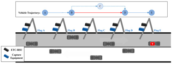
Figure 4.
Schematic diagram of missing detection pattern.
The leakage detection rate is defined as follows:
where denotes the total number of missing detections and denotes the total number of transaction records.
It should be noted that a missing transaction signifies the presence of a pair of neighboring gantries that are connected but have a Dijkstra path distance greater than 2 within a trip trajectory. In other words, a Missing Detection can result in the omission of one or more gantries. Multiple missing detections can occur within a single trip trajectory.
- (3)
- Opposite Lane Detection
Opposite lane detection refers to a situation in which a vehicle passing through a gantry is mistakenly detected by the opposing lane, leading to the generation of inaccurate data. This may occur due to various factors, including unusual weather conditions and equipment misalignment angles. In Figure 5, a schematic representation of opposite lane detection is depicted, where a vehicle passing through gantry B is erroneously detected by the opposing lane B’, resulting in the production of erroneous data.
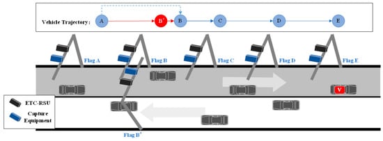
Figure 5.
Schematic diagram of opposite lane detection pattern.
The opposite lane detection rate is defined as follows:
where denotes the total number of opposing detections and denotes the total number of transaction records. It should be noted that there may be more than one pairwise detection in a trip track.
- (4)
- Duplicate Detection
Duplicate detection is the occurrence where a vehicle passing through a gantry is mistakenly detected twice, leading to the generation of two sets of data. Figure 6 presents a schematic illustration of duplicate detection, where the vehicle is detected twice by gantry B, resulting in the creation of redundant data.
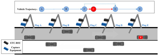
Figure 6.
Schematic diagram of duplicate detection pattern.
The duplicate detection rate is defined as follows:
where denotes the total number of duplicate detections and denotes the total number of transaction records. It should be noted that there may be more than one repeat detection in a trip track.
4. Method
4.1. Problem Description
Within expressway ETC big data, there is a presence of abnormal data, which exhibits various types and intricate information. This study constructs the expressway data into a segment trajectory table, utilizing this table as the model input to determine whether the segment trajectory is normal or falls under one of several potential abnormalities. Our exploratory analysis indicates the potential existence of four types of abnormalities within the segment trajectory, effectively framing the problem as a multi-classification challenge.
The vehicle’s travel trajectory can be represented as a unidirectional chain table, denoted as , where indicates the number of the gates passing through. For a correct and complete ordinary vehicle travel track, the first node of the chain table should be the entrance toll station or the exit gateway, and the last node of the chain table should be the exit toll station or the exit gateway, and the distance between any neighboring nodes (without distinguishing whether they are the first and last nodes or not) in the expressway network topology is 1.
In the chain table generated by an abnormal trip, the neighboring nodes in the expressway network topology may be unconnected or connected, but the distance between the two nodes is not equal to 1. This study presents a model designed to automatically identify anomalies within a trip. However, in the actual trip trajectory, more than 1 anomaly may occur in a trip. In order to accurately locate where the anomaly occurs and to simplify the model, in the model design, the chain table is split into chain lists for storing section trips, which are all of length 2, e.g., , , , and each section track uniquely belongs to a trip trajectory and has a unique anomaly state, i.e., a pair of gantries can only possibly be a normal mode or there exists a certain abnormal mode, and a model can be constructed for directly determining the mode to which a gantry pair belongs.
4.2. Tomek-Links Resampling Algorithm
The 773,281 trajectories with anomalies on a certain day are divided into 5,532,577 zonal trajectory sets, and the normal rate, reverse trajectory rate, missing detection rate, opposite detection rate, and repeated detection rate are calculated, respectively, and the statistical results are shown in Figure 7. It can be seen that there is a serious imbalance in the dataset, which is not conducive to model training. Therefore, it is necessary to resample the dataset before model training.
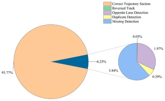
Figure 7.
Percentage of data categories.
On a specific day, the 773,281 trajectories exhibiting anomalies are categorized into 5,532,577 sets of section trajectories. Subsequently, we compute the rates for normal trajectories, reverse trajectories, missing detection, opposite lane detection, and duplicated detection. The statistical findings are presented in Figure 7. It is evident that the dataset suffers from a significant imbalance, which hinders effective model training. To address this, dataset resampling is deemed necessary before proceeding with model training.
Resampling algorithms can be specifically categorized as oversampling and undersampling. Undersampling algorithms balance the number of positive and negative samples by deleting the majority class samples. Oversampling methods address class imbalance by generating additional minority class samples. Tiancheng Li et al. [34] used a mixture of probabilistic sampling and systematic sampling in the particle filtering process to prevent particle degradation and depletion. Jin Xiao et al. [35] used a fusion of multiple resampling algorithms to improve the effectiveness of classification models. The effect of the classification model is improved. Upon conducting exploratory analysis, we observed three distinctive characteristics in the expressway anomalous pattern data:
- Severe class imbalance: The number of samples for anomalous patterns is notably small.
- Predominance of normal data: A majority of samples belong to the normal data category with a large number of similar samples.
- Clear separation between normal pattern samples and samples from each anomalous pattern category.
Therefore, we employ an undersampling algorithm to address these data imbalances before model training. The Tomek-links algorithm show in Algorithm 4, a classical undersampling technique, is chosen for its ability to effectively reduce the number of majority class samples near the class boundary without sacrificing essential data information. This process eliminates noisy data in the boundary of the majority class, ultimately enhancing class separation and improving classifier performance. The characteristics of the Tomek-links algorithm align with the characteristics of the expressway anomaly pattern data, making it a suitable choice for undersampling in this study.
The algorithm takes one minority class sample at a time and pairs it with a majority class sample. If there are multiple minority class samples, the process is repeated. It pairs the first minority class sample with the first majority class sample and continues until all minority class samples have been processed.
The algorithm operates on the assumption that if two samples from different categories are each other’s nearest neighbors, it suggests that one of the samples may be noise or both samples are situated on the category boundary. Tomek links consist of pairs of samples that connect majority category samples with minority category samples in the feature space. Specifically, Tomek links are defined by the condition that for each sample, its nearest neighbors belong to different categories, forming pairs known as members of a Tomek link.
The algorithm’s process is illustrated in Figure 8. In Figure 8a, you can see the original dataset, containing three categories of samples, with circles representing majority category samples. For each majority category sample, its nearest neighbor is identified, as shown in Figure 8b. If that nearest neighbor is a minority category sample, the pair is considered a member of a Tomek link. The members of the Tomek link are then removed from the dataset, effectively eliminating the connection between the majority category sample and the minority category sample. These steps are repeated until no more new Tomek links can be identified, resulting in the dataset shown in Figure 8c. Ultimately, a new dataset is obtained, which is a subset of the original dataset, as illustrated in Figure 8d.
| Algorithm 4: Tomek Links |
| 1. Input: majority_samples, minority_sample 2. Initialize: found_new_link = True 3. while found_new_link: 4. found_new_link = False 5. for majority_sample in majority_samples do 6. closest_distance = float(‘inf’) 7. closest_minority_sample = None 8. for minority_sample in minority_samples do 9. distance = pairwise_distances(majority_sample, minority_sample) 10. if distance < closest_distance do 11. closest_distance = distance 12. closest_minority_sample = minority_sample 13. if closest_minority_sample is not None do 14. found_new_link = True 15. majority_samples.remove(majority_sample) 16. minority_samples.remove(closest_minority_sample) |
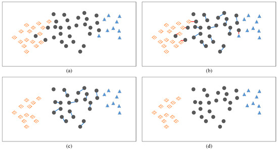
Figure 8.
Schematic diagram of the Tomek-links algorithm: (a) original data, (b) finding Tomek links, (c) removing eligible Tomek links, (d) new dataset.
4.3. Feature Vector Modeling
In anomaly pattern analysis, we design feature vectors from three perspectives: spatial, temporal, and travel, respectively.
- Spatial Characteristics:
The spatial feature spatial set encompasses the gantry number and its type, both of which reflect the correctness of the section, its location, and its relationship within the expressway network topology. The representation is as follows:
where and denote the gantry number and and denote the type of gantry. The details are as follows:
- Origin gantry number and destination gantry number
Each gantry on a Chinese expressway is assigned a unique number that reflects its precise location. The pair of gantry numbers ( and ) helps determine the specific section through which a vehicle passes. In normal data, this gantry number pair accurately represents the section, whereas in abnormal data, the gantry numbers may not correctly represent the section.
- Origin Gantry Type and Destination Gantry Type
Gantry types on the expressway include road section gantries, provincial boundary entrance gantries, provincial boundary exit gantries, entrance toll station gantries, and exit toll station gantries. These types provide information about the gantries’ locations within the expressway network topology. represents the gantry type at the starting point, and indicates the gantry type at the end point.
- 2.
- Time Characteristics:
The time feature includes the gantry transaction time and the section passage time and is expressed as follows:
where and denote the transaction time of the vehicle passing through the starting gantry and the ending gantry, respectively, and denotes the sectinon passage time, which is represented by a timestamp. denotes the section passage time, which is the time difference between the transaction time of passing through the starting gantry and the ending gantry, in seconds, and is computed by the following formula:
- Travel Characteristics
Travel Characteristics travel includes the trip code and trip length. The denotation is as follows:
where denotes the trip code and denotes the trip length. Specifically, in the expressway ETC system, each trip has a unique code that is not duplicated and does not change midway. The trip length is the total number of gantries passed in that trip.
4.4. Expressway ETC Data Anomaly Pattern Recognition Model Based on TL-XGBoost
XGBoost, a tree-based data classification algorithm that has gained significant popularity in recent years, is known for its efficiency in handling unbalanced datasets [36]. However, it tends to underperform in terms of recall when dealing with such datasets. In this study, we combine the Tomek-links (TL) algorithm with XGBoost to create a robust model for recognizing expressway ETC data anomaly patterns, referred to as TL-XGBoost. The model framework is depicted in Figure 9.
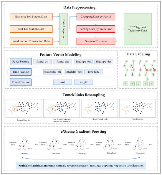
Figure 9.
Expressway ETC data anomaly pattern recognition model framework based on TL-XGBoost.
XGBoost, an ensemble learning method based on boosting algorithms, offers an efficient implementation of the Gradient Boosting Decision Tree (GBDT) algorithm. It employs decision tree models iteratively to generate new trees and learns the residuals between true and currently predicted values of all trees. The final result is accumulated from all the trees, leading to improved classification accuracy. By utilizing the XGBoost algorithm as a classifier for recognizing anomalous patterns in expressway transaction data, precise anomalous pattern classification can be achieved.
From data with known anomaly types, we extract nine-dimensional feature vectors to create a sample dataset, which is denoted as . Here, represents the nine-dimensional feature vector of expressway transaction data anomalies, while represents the labeled value indicating the data anomaly pattern corresponding to .
Assuming that the XGBoost integrated learning model integrates K classification trees, the classification result of the XGBoost algorithm can be expressed as follows:
where k is the number of trees, corresponds to the kth classifiable tree, and is the integrated classifier consisting of all classified trees.
The objective function of XGBoost consists of a loss function and a regularization term aimed at preventing overfitting. It employs techniques like L1 and L2 regularization as well as subsampling and column sampling to control model complexity and enhance generalization. L1 regularization promotes sparsity in model parameters, while L2 regularization prevents overfitting. Subsampling and column sampling help reduce variance and improve model robustness. Including the regularization term in the objective function enhances the model’s robustness during training. The objective function of XGBoost can be expressed as shown below:
where is the number of trees and is a regularization parameter to control the number of trees.
Classification problems usually use a logistic loss function:
To extend the logistic loss function for multi-classification, the softmax function can be applied to transform the predictions of a multiclass problem into a probability distribution. Subsequently, the cross-entropy loss function can be employed to assess the disparity between the predicted results and the true labels. The cross-entropy loss function can be expressed as:
where is the label (0 or 1) of the th sample belonging to the th category, and is is the value of the predicted probability that the ith sample belongs to the th category (∈[0,1]).
The XGBoost algorithm employs an additive stepwise integration strategy during training. It optimizes the first tree, then the second tree, and continues until the th tree is optimized, resulting in a continuous reduction in the loss function during the optimization process. The prediction accuracy is enhanced by introducing the incremental function to optimize the objective function throughout the iteration process. The calculation method can be expressed using the equation in the following formula:
Expanding the second-order Taylor’s equation and removing the constant term results in a reduction in the model’s runtime, which is expressed as follows:
Finally, the hyperparameters of XGBoost, such as the learning rate, the number of decision trees, maximum depth, etc., are optimized to achieve the best results.
5. Experiment
The experimental platform is built on an AMD Ryzen 7 5800H with Radeon Graphics running at 3.20 GHz and equipped with 16 GB of RAM. The experiments were performed using the Windows 11 (Core) operating system and the Python 3.10.11 programming language. The experimentation was conducted within Jupyter Lab, an interactive programming IDE. For additional details about Jupyter Lab, please visit its official website: “https://jupyter.org/ (accessed on 15 November 2023)”.
5.1. Evaluation Indicators
Following common evaluation methods for multicategorization problems [37], this paper employs four evaluation metrics to comprehensively assess the model’s performance. These metrics are Accuracy, Precision, Recall, and F1-score.
Accuracy: Accuracy is one of the most commonly used evaluation metrics in classification models. It represents the proportion of correctly predicted samples out of the total number of samples.
Precision measures the proportion of samples predicted by the model to be positive classes that are actually positive classes. A high precision rate indicates that the model is better at recognizing positive classes.
Recall measures the model’s ability to identify positive class samples, which is also known as sensitivity or the true positive rate. As shown in Equation (21), it calculates the percentage of samples that the model correctly predicts as the positive class. A high recall rate indicates that the model is better at recognizing the positive class.
The F1-score is the reconciled mean of precision and recall and is used to comprehensively assess the performance of a classification model. It combines the model’s precision in samples predicted to be positively classified and its recall for positively classified samples. A higher F1-score indicates that the model strikes a better balance between precision and recall.
5.2. Data Preprocessing and Resampling
The experimental data employed in this study are sourced from the ETC transaction records of an expressway located in a southeastern province specifically for a single date in June 2021. From the province’s records on that particular date, approximately 63,381 ETC data entries were selected for analysis. This dataset is partitioned into a training set, constituting 80% of the data, and a test set, which encompasses the remaining 20%.
5.2.1. Data Encoding and Labeling
In the field of machine learning, a significant number of algorithms, including XGBoost, decision trees, and random forests, primarily process numerical data and are not inherently compatible with character-based data. Nevertheless, real-world datasets often consist of labels and features that are initially represented in a non-numeric format following data collection. To accommodate such data within the algorithms, encoding is required, effectively translating character-based information into a numeric representation. This transformation enables the seamless integration of diverse data types into machine learning models for analysis and prediction.
Within the expressway ETC dataset, several features encompass date and time-related information, notably section origin time, section destination time, and the time delta representing a vehicle’s passage through a section. Originally recorded in date–time format, these attributes were subjected to a transformation, converting them into integer timestamps.
Furthermore, specific categorical variables such as gantry number, gantry type, and trip number were initially documented in non-standard or extended string formats. To render them amenable to analysis, these categorical variables underwent encoding via the LabelEncoder technique. This process mapped them to numeric representations, such as , for enhanced computational compatibility. An example of these encoded data can be found in Table 9 for reference.
Table 9.
Example of data encoding results.
Labeling is a pivotal component of supervised learning, and the labeling process for the expressway ETC anomaly dataset in this study follows these key steps. Initially, the abnormal patterns within the ETC trajectories are labeled through the application of Algorithm 3. Subsequently, the ETC trajectories are partitioned into multiple section trajectory chain lists, with each list being explicitly associated with a specific type of abnormality pattern. Lastly, the section trajectory chain lists are labeled by merging them with labeled ETC trajectories. The label design is presented in Table 10 for reference.
Table 10.
Dataset labels.
5.2.2. Feature Vector Construction
Based on the feature vector model we developed, we created a feature vector dataset for identifying expressway anomaly data. Examples of these feature vectors are provided in Table 11.
Table 11.
Expressway abnormal data feature vector set example.
We conducted a correlation analysis on these features with the results displayed in Figure 10.
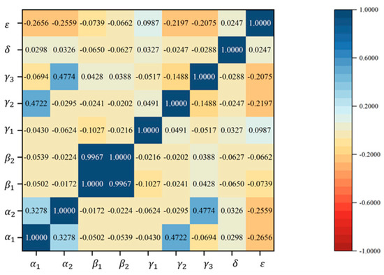
Figure 10.
Feature correlation analysis chart.
The correlation between the gantry number at the beginning of the section and the gantry number at the end of the section is 0.3278, indicating a positive but not particularly strong correlation. The relationship between gantry nodes is complex, involving both back-and-forth movements, diversions, and mergers. This non-linearity affects the correlation.
The correlation between the timestamps of vehicles passing through the gantries at the beginning of the section and of vehicles passing through the gantries at the end of the section is nearly 1.0, suggesting a very strong correlation. However, their correlation with the time of passage through the section is low, implying that provides distinct information.
The correlation between the gantry types, at the beginning of the section and at the end, is −0.148796, indicating an inverse relationship. These features represent gantry types, and a section start gantry being the provincial boundary entrance gantry or entrance toll station gantry must lead to the section end gantry being the road section gantry, provincial boundary exit gantry, or exit toll station gantry. Since provincial boundary and toll station gantries appear less frequently, and road section gantries are more common, the absolute value of this correlation is smaller.
Correlations between and , as well as and , are higher due to the likelihood of a section start gantry being a provincial boundary entrance or entrance toll station gantry and a section end gantry being an exit provincial boundary or exit toll station gantry.
In contrast, features and represent information in the trip trajectory dimension, and their correlations with other features are low due to the differing types of information they provide.
5.2.3. Resampling
In this study, the degree of improvement on the training effect of machine learning models and the sampling time are used to evaluate the resampling effect. The Tomek-links algorithm is used to resample the training set data and is compared with two other undersampling algorithms, namely random undersampling and the CNN (Condensed Nearest Neighbor Rule) undersampling algorithm. This section is intended to discuss the performance of the resampling algorithms. To control the variables and focus on the comparison of the resampling algorithms, the XGBoost model is used with default parameters, and the random seed is set to 42.
The impact of resampling on the time consumption of the model building process is analyzed in Table 12. Specifically, the CNN algorithm requires significantly more time than other algorithms, totaling 12,694.98 s, which is equivalent to approximately 3.5 h. In contrast, resampling using the Tomek-links and random resampling methods takes less than 1 s.
Table 12.
Comparison of resampling algorithms.
Furthermore, the Tomek-links algorithm effectively mitigates the class imbalance issue without substantially reducing the dataset’s size, as observed with random resampling. Preserving the dataset’s size can be advantageous in scenarios where the original dataset’s model training time is acceptable, as it helps retain more feature information and maintain better generalization. Taking both time efficiency and dataset quality into account, the Tomek-links algorithm is better suited to meet the goals of this study.
We also employed the XGBoost model to train and test the resampled dataset, and the results are presented in Figure 11. In the evaluation of three key metrics, namely Accuracy, Precision, and F1-score, the dataset resampled using the Tomek-links algorithm outperformed not only the original dataset but also other resampled datasets, securing the top position. Specifically, in terms of Recall, the dataset obtained through Tomek-links resampling achieved the second-highest ranking, which is second only to the random undersampling dataset. In summary, the Tomek-links resampling approach demonstrated superior effectiveness.
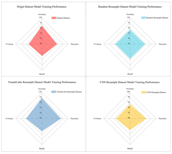
Figure 11.
Model training performance on resampled datasets.
5.3. Parameter Optimization
Parameter selection plays a crucial role in influencing the performance of machine learning models. Optimal parameter choices can enable a model to attain its highest level of performance. As such, the parameter selection and optimization process for XGBoost represent a vital step in this study. We undertake parameter tuning through the grid search method, focusing on four primary categories of parameters: general parameters, parameters related to tree structure, parameters related to sample randomization, and regularization parameters.
General parameters encompass ‘learning_rate’ and ‘n_estimators’, both of which directly impact the model’s learning capacity and training speed. ‘Learning_rate’ determines the step size for model updates in each iteration, while ‘n_estimators’ sets the number of iterations for model training, signifying the quantity of weak learners (decision trees) generated.
Tree structure-related parameters consist of ‘max_depth’, ‘min_child_weight’, and ‘gamma’. ‘Max_depth’ dictates the maximum depth of each decision tree, ‘min_child_weight’ specifies the minimum sum of weights for each leaf node, and ‘gamma’ controls the minimum loss reduction required for leaf node splitting. These parameters collectively regulate the complexity of the decision tree and significantly influence the model’s performance and generalization capability.
Random sampling-related parameters include ‘subsample’ and ‘colsample_bytree’, governing the proportion of randomly selected samples and features, respectively, within the training set. Appropriate settings for these parameters enhance model diversity and mitigate overfitting risks.
Regularization parameters, namely ‘reg_alpha’ (L1 regularization parameter) and ‘reg_lambda’ (L2 regularization parameter), are utilized to manage model complexity and prevent overfitting.
The specific parameter settings are shown in Table 13.
Table 13.
Optimized hyperparameter settings.
The comparison between the model’s performance with default parameters and the model utilizing optimal parameters is depicted in Figure 12.
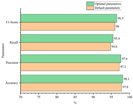
Figure 12.
Parameter optimization effect.
5.4. Experimental Result and Evaluation
To evaluate the performance of various machine learning algorithms for the task of expressway transaction data anomaly pattern recognition and validate the expressway transaction data anomaly pattern recognition model based on TL-XGBoost, we conducted a series of experiments. In addition to evaluating XGBoost for comparison, we also assessed several other machine learning algorithms, including Light Gradient Boosting Machine (LightGBM), CatBoost, decision tree (DT), and random forest (RF), comparing their performance with the XGBoost algorithm. Default parameters were used for these algorithms during training, and the random seed was set to 42.
The experiments demonstrate that TL-XGBoost, as proposed in this paper, outperforms both the traditional XGBoost method [38] and other machine learning algorithms. The other classification methods mentioned earlier have their own strengths and limitations, and TL-XGBoost is selected as the preferred choice because it effectively addresses many of the limitations found in existing models. There are two primary reasons for choosing TL-XGBoost as the preferred classification model for the task of classifying anomalous patterns in expressway ETC data. On the one hand, the XGBoost algorithm offers several advantages:
- High Accuracy: XGBoost is known for its ability to provide superior accuracy compared to many other algorithms. It achieves this by gradually improving the model through multiple rounds of iterations;
- Regularization Support: XGBoost supports both L1 and L2 regularization, which aids in reducing the risk of overfitting. Regularization techniques help control the model’s complexity and enhance its generalization capabilities;
- Hyperparameter Tuning: XGBoost provides a rich set of hyperparameters that can be fine-tuned to optimize the model for different tasks. These parameters include tree depth, learning rate, regularization, and more;
- High Performance: XGBoost is highly optimized, incorporating advanced techniques such as tree pruning, sparsity awareness, cache blocks, and parallel processing. This optimization allows XGBoost to deliver fast training and prediction, even on large-scale datasets, making it well suited for real-world applications.
On the other hand, the Tomek-links algorithm effectively addresses issues related to low recall and the imbalance in decision boundaries resulting from sample imbalance. Consequently, the TL-XGBoost model, which combines the Tomek-links algorithm with the XGBoost algorithm, demonstrates excellent performance.
Referring to Figure 13, it is evident that the TL-XGBoost model outperforms all other models across all four metrics, including Accuracy, Precision, Recall, and F1-score. Notably, the improvements in Precision and F1-score metrics are particularly significant when compared to the performance of the XGBoost model.
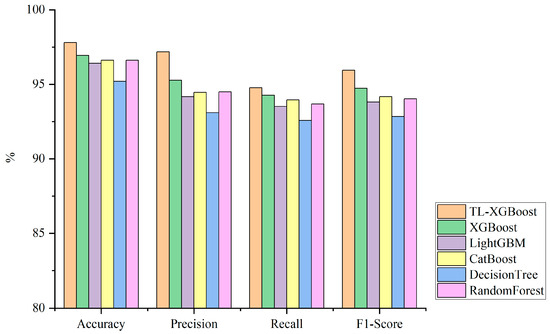
Figure 13.
Comparison of algorithm performance.
Subsequently, a detailed feature contribution analysis was conducted. As depicted in Figure 14, the two features exhibiting the highest feature contributions are the section start gantry type and the section passage time, representing the spatial and temporal attributes of section trajectories, respectively. It is noteworthy that none of the feature contribution values surpass 0.5. This indicates that every feature makes a discernible contribution to the model’s predictive outcomes, and no single feature overwhelmingly influences the model’s predictive results.
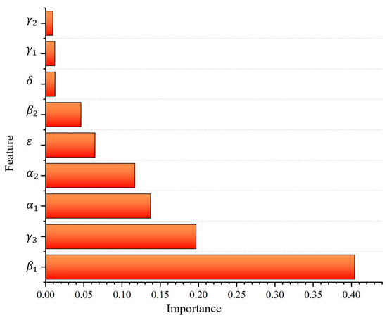
Figure 14.
Feature importance.
5.5. Expressway ETC Data Anomaly Pattern Analysis
This section delves into the causes behind four anomalous patterns: reverse trajectory, missing detection, duplicate detection, and opposite lane detection. Following this analysis, we examine the potential impact of these anomalies on the safety of the vehicle–road coordination system.
- Reverse trajectory patterns
In our dataset, we identified anomalous data featuring reverse trajectory patterns within 30 section trajectories. Upon close examination, and considering the original gantry serial numbers and topology data, our initial hypothesis attributes this anomaly to potential misconfigurations during the installation and commissioning of the gantry system. These configuration errors may have led to discrepancies between the internal gantry equipment numbering and the designated numbering in the topology data, ultimately resulting in the generation of reverse trajectories during vehicle trajectory recording.
- 2.
- Missing Detection Patterns
Regarding the missing detection patterns in our dataset, we conducted an analysis from two distinct angles. Firstly, we examined cases characterized by a significant number of missing detections at individual gantries. This scrutiny revealed a total of 893 missing detections. Three gantries had over 1000 missing detections, while 55 gantries had more than 100 missing detections. Our initial speculations regarding these findings encompass three potential factors:
- Mechanical Abnormalities: It is possible that these gantries suffered mechanical irregularities or angular misalignments necessitating maintenance;
- Malicious Electromagnetic Shielding: The deliberate placement of electromagnetic shielding objects near gantry equipment to evade detection could be another explanation.
- Atmospheric Conditions: Adverse weather conditions on the specific day in question, such as temperature and humidity fluctuations, might have deteriorated signal quality.
Secondly, we find that there are 16 sets of trajectories with four or more consecutive missing detections of gantries that occur more than 10 times in the same day. The trajectory with the highest number of consecutively missing detections, as shown in Figure 15, has a total of 39 consecutive missing detections. In such cases, the possible causes speculated in the first scenario should be eliminated first. If no relevant problem is identified, two alternative explanations are considered:
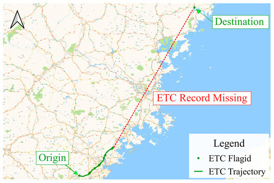
Figure 15.
An example of ETC trajectory with missing detection.
- Abnormal OBU Equipment: Mechanical anomalies in the On-Board Unit (OBU) equipment of certain vehicles might have occurred, coinciding with their passage on the relevant road that day.
- Fee Evasion Suspicions or Inaccurate Fee Calculations: The patterns observed in these travel tracks may give rise to suspicions of potential fee evasion or inaccurate system fee calculations.
- 3.
- Repeated Detection Patterns
In the dataset we used, there were 185 gantries with repeated detection patterns and 7 gantries with more than 100 repeated detections. We initially speculate that these may be due to the following reasons:
- Abnormalities in Gantry Equipment: The presence of repeated detections in some gantries may indicate abnormalities in these specific gantries. Professionals may need to re-commission and inspect the affected equipment.
- Roadway Issues: There are other problems in the roadway on the same day that lead to poor access.
- 4.
- Opposite Lane Detection Patterns
In the dataset we used, there were a total of 388 gantries exhibiting opposite lane detection patterns, and one gantry had more than 150 opposing lane detections. Our initial hypothesis is that this anomaly may be linked to a shifted installation angle of the gantry equipment, necessitating professional adjustment.
The core task of the vehicle–road collaboration system is to comprehensively assess the road traffic condition and instantly share the assessment results with all intelligent driving vehicles in order to warn of potentially hazardous situations and help vehicles avoid them in advance [39].
Abnormal patterns can significantly impact the vehicle–road cooperative system in the following ways. First, in the roadway with a high frequency of missed detection patterns or repeated detection, it will increase the error of the traffic state assessment results, which in turn will cause misleading path planning for a single vehicle.
Second, the reverse trajectory and continuous missed detection mode will affect the real-time vehicle position estimation, vehicle arrival time prediction, and prediction of low-speed vehicles in front versus high-speed vehicles behind.
For example, in Figure 15, a vehicle has a large number of consecutive missed detections during that trip. Figure 16 tries to complement that trajectory, where the red color represents the shortest path, while the blue color depicts the actual reconstructed trajectory of the vehicle based on captured data, exhibiting variations from the two trajectories. In segments where captured data diverge from the shortest path trajectory, the travel distances differ significantly, spanning 26.9845 km and 34.5718 km, respectively, and encompassing approximately 20 gantries each. Within these road sections, accurately calculating the vehicle’s position and state in real time becomes challenging. If the vehicle is traveling at excessively high or low speeds, it could potentially pose a road hazard that intelligent driving systems may fail to anticipate, thereby compromising driving safety.
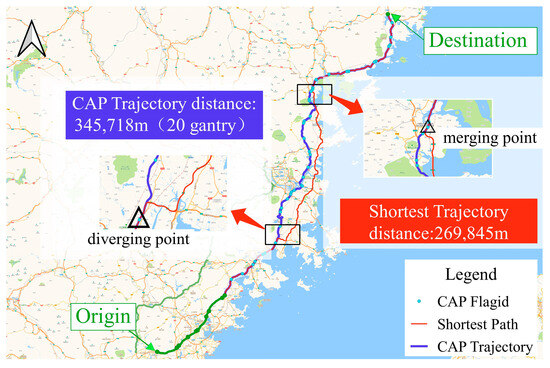
Figure 16.
An example of ETC trajectory repair. Note that CAP trajectory and shortest trajectory distances are calculated only for the distance traveled between the diverging point and the merging point, not for the total length of the travel trajectory.
Third, the road sections with frequent opposite direction detection and reverse trajectory patterns will interfere with the system’s judgment of road connectivity.
In conclusion, detecting and identifying abnormal patterns in expressway ETC data is crucial. Improving the quality of these data will offer more reliable support for the ETC-based vehicle–road cooperative system.
6. Discussion
China’s expressway ETC system has been widely used, and the realization of cooperative vehicle–infrastructure based on the expressway ETC system is advanced and feasible. The correctness of the ETC data, as the data support of this scheme, will directly affect the safety of driving. Research on abnormal data in expressway ETC data is the basis for improving data quality. In this study, an investigation into abnormal data within expressway ETC datasets has led to the following main contributions and innovations:
- Classification of Abnormal Data: Unlike previous approaches that often involved simplistic interpolation or direct data deletion during data preprocessing, this study introduces a classification of abnormal data within expressway ETC big data. By doing so, it provides a reference for the more precise and rational repair of abnormal data, resulting in the construction of more complete and comprehensive datasets;
- Robust Anomaly Pattern Recognition Model: The study proposes an accurate and comprehensive expressway anomaly pattern recognition model capable of identifying four distinct types of anomalies within extensive ETC big data. This model achieves exceptional performance metrics with an accuracy of 97.8%, precision of 97.2%, recall of 94.7%, and F1-score of 96.0%.
- Analysis of Anomalous Patterns: The research delves into four primary types of anomalous patterns—reverse trajectory, missing detection, false detection, and repeated detection. Speculations on potential causes for each type of anomaly are provided, offering valuable insights and directions for future research.
In the future, efforts can be focused on two aspects: firstly, enhancing the model’s accuracy further to facilitate its application in the cooperative vehicle–infrastructure platform based on the ETC system; and secondly, conducting repairs on existing anomalies and further exploration of potential anomaly patterns within ETC data
Author Contributions
Conceptualization, F.Z., R.S. and Y.L.; methodology, R.S., Y.L. and Z.H.; software, R.S., Y.L. and Z.H.; validation, R.S., H.Z. and F.Z.; formal analysis, R.S. and Z.H.; investigation, H.Z. and W.W.; resources, F.Z.; data curation, Z.H., H.Z. and W.W.; writing—original draft preparation, R.S.; writing—review and editing, F.Z. and Y.L.; visualization, R.S.; supervision, F.Z. and Y.L.; project administration, F.Z. and R.S.; funding acquisition, F.Z. All authors have read and agreed to the published version of the manuscript.
Funding
This work is partially supported by the Key Technologies Innovation and Industrialization Project (Funding number: 2023XQ008), the Renewable Energy Technology Research institution of Fujan University of Technology Ningde, China (Funding number: KY310338), the 2020 Fujian Province “Belt and Road” Technology Innovation Platform (Funding number: 2020D002), The Construction Project of the Intelligent Networking Research Institute of Fujian University of Engineering (Funding number: GY-Z23012), the Provincial Candidates for the Hundred, Thousand and Ten Thousand Talent of Fujian (Funding number: GY-Z19113), the Patent Grant project (Funding numbers: GY-Z18081, GY-Z19099, GY-Z20074, GY-Z23050), Horizontal projects (Funding number: GY-H-20077), Municipal level science and technology projects (Funding numbers: GY-Z-22006, GY-Z-220230), Fujian Provincial Department of Science and Technology Foreign Cooperation Project (Funding number: 2023I0024), the Open Fund project (Funding number: KF-19-22001).
Institutional Review Board Statement
Not applicable.
Data Availability Statement
The ETC transaction data utilized in this study were obtained from Fujian Expressway Information Technology Co., Ltd. (Fuzhou, China). Restrictions apply to the availability of these data, which were used under license for this study and are not publicly available. Data are available from the authors with the permission of Fujian Expressway Information Technology Co., Ltd. All data processing and analyses were conducted in compliance with relevant data protection and privacy laws. No individual or personal data were used in this study.
Conflicts of Interest
Author Yongyu Luo was employed by the company Fujian Provincial Expressway Information Technology Co., Ltd. The remaining authors declare that the research was conducted in the absence of any commercial or financial relationships that could be construed as a potential conflict of interest.
References
- Wu, D.; Guan, Y.; Xia, X.; Du, C.; Yan, F.; Li, Y.; Hua, M.; Liu, W. Coordinated Control of Path Tracking and Yaw Stability for Distributed Drive Electric Vehicle Based on AMPC and DYC. arXiv 2023, arXiv:2304.11796. [Google Scholar]
- Li, S.; Li, Z.; Yu, Z.; Zhang, B.; Zhang, N. Dynamic Trajectory Planning and Tracking for Autonomous Vehicle with Obstacle Avoidance Based on Model Predictive Control. IEEE Access 2019, 7, 132074–132086. [Google Scholar] [CrossRef]
- Meng, Z.; Xia, X.; Xu, R.; Liu, W.; Ma, J. HYDRO-3D: Hybrid Object Detection and Tracking for Cooperative Perception Using 3D LiDAR. IEEE Trans. Intell. Veh. 2023, 8, 4069–4080. [Google Scholar] [CrossRef]
- Chen, S.; Hu, J.; Shi, Y.; Zhao, L.; Li, W. A Vision of C-V2X: Technologies, Field Testing, and Challenges with Chinese Development. IEEE Internet Things J. 2020, 7, 3872–3881. [Google Scholar] [CrossRef]
- Saad, M.M.; Khan, M.T.R.; Shah, S.H.A.; Kim, D. Advancements in Vehicular Communication Technologies: C-V2X and NR-V2X Comparison. IEEE Commun. Mag. 2021, 59, 107–113. [Google Scholar] [CrossRef]
- Chen, C.; Yao, G.; Liu, L.; Pei, Q.; Song, H.; Dustdar, S. A Cooperative Vehicle-Infrastructure System for Road Hazards Detection with Edge Intelligence. IEEE Trans. Intell. Transport. Syst. 2023, 24, 5186–5198. [Google Scholar] [CrossRef]
- Cai, L.; Meng, C.; Wang, X.; Lyu, C.; Sun, X. Cooperative Vehicle-Infrastructure System Use Case Design for Smart Highway. In Proceedings of the 2020 7th International Conference on Information Science and Control Engineering (ICISCE), Changsha, China, 18–20 December 2020; pp. 415–421. [Google Scholar]
- Zou, F.; Guo, F.; Luo, S.; Liao, L.; Li, N.; Xing, Y. Research and Design of ETC Simulation Platform for Expressway. J. Syst. Simul. 2023, 35, 2624–2640. [Google Scholar]
- Zou, F.; Ren, Q.; Tian, J.; Guo, F.; Huang, S.; Liao, L.; Wu, J. Expressway Speed Prediction Based on Electronic Toll Collection Data. Electronics 2022, 11, 1613. [Google Scholar] [CrossRef]
- Cai, Q.; Yi, D.; Zou, F.; Zhou, Z.; Li, N.; Guo, F. Recognition of Vehicles Entering Expressway Service Areas and Estimation of Dwell Time Using ETC Data. Entropy 2022, 24, 1208. [Google Scholar] [CrossRef]
- Wang, H.; Zou, F.; Tian, J.; Guo, F.; Cai, Q. Analysis on Lane Capacity for Expressway Toll Station Using Toll Data. J. Adv. Transp. 2022, 2022, 9277000. [Google Scholar] [CrossRef]
- Guo, F.; Zou, F.; Luo, S.; Liao, L.; Wu, J.; Yu, X.; Zhang, C. The Fast Detection of Abnormal ETC Data Based on an Improved DTW Algorithm. Electronics 2022, 11, 1981. [Google Scholar] [CrossRef]
- Quatrini, E.; Costantino, F.; Di Gravio, G.; Patriarca, R. Machine Learning for Anomaly Detection and Process Phase Classification to Improve Safety and Maintenance Activities. J. Manuf. Syst. 2020, 56, 117–132. [Google Scholar] [CrossRef]
- Chandola, V. Anomaly Detection: A Survey. ACM Comput. Surv. 2009, 41, 1–58. [Google Scholar] [CrossRef]
- Rousseeuw, P.J.; Hubert, M. Anomaly Detection by Robust Statistics. WIREs Data Min. Knowl. Discov. 2018, 8, e1236. [Google Scholar] [CrossRef]
- Jain, M.; Kaur, G.; Saxena, V. A K-Means Clustering and SVM Based Hybrid Concept Drift Detection Technique for Network Anomaly Detection. Expert Syst. Appl. 2022, 193, 116510. [Google Scholar] [CrossRef]
- Lei, L.; Wu, B.; Fang, X.; Chen, L.; Wu, H.; Liu, W. A Dynamic Anomaly Detection Method of Building Energy Consumption Based on Data Mining Technology. Energy 2023, 263, 125575. [Google Scholar] [CrossRef]
- Chen, L.; Gao, S.; Liu, B. An Improved Density Peaks Clustering Algorithm Based on Grid Screening and Mutual Neighborhood Degree for Network Anomaly Detection. Sci. Rep. 2022, 12, 1409. [Google Scholar] [CrossRef]
- Cauteruccio, F.; Cinelli, L.; Corradini, E.; Terracina, G.; Ursino, D.; Virgili, L.; Savaglio, C.; Liotta, A.; Fortino, G. A Framework for Anomaly Detection and Classification in Multiple IoT Scenarios. Future Gener. Comput. Syst. 2021, 114, 322–335. [Google Scholar] [CrossRef]
- Tama, B.A.; Comuzzi, M.; Rhee, K.-H. TSE-IDS: A Two-Stage Classifier Ensemble for Intelligent Anomaly-Based Intrusion Detection System. IEEE Access 2019, 7, 94497–94507. [Google Scholar] [CrossRef]
- Zhang, L.; Su, H.; Zio, E.; Zhang, Z.; Chi, L.; Fan, L.; Zhou, J.; Zhang, J. A Data-Driven Approach to Anomaly Detection and Vulnerability Dynamic Analysis for Large-Scale Integrated Energy Systems. Energy Convers. Manag. 2021, 234, 113926. [Google Scholar] [CrossRef]
- Au Yeung, J.F.K.; Wei, Z.; Chan, K.Y.; Lau, H.Y.K.; Yiu, K.-F.C. Jump Detection in Financial Time Series Using Machine Learning Algorithms. Soft Comput. 2020, 24, 1789–1801. [Google Scholar] [CrossRef]
- Su, Y.; Zhao, Y.; Niu, C.; Liu, R.; Sun, W.; Pei, D. Robust Anomaly Detection for Multivariate Time Series through Stochastic Recurrent Neural Network. In Proceedings of the 25th ACM SIGKDD International Conference on Knowledge Discovery & Data Mining, Anchorage, AK, USA, 4–8 August 2019; Association for Computing Machinery: New York, NY, USA, 2019; pp. 2828–2837. [Google Scholar]
- Li, J.; Izakian, H.; Pedrycz, W.; Jamal, I. Clustering-Based Anomaly Detection in Multivariate Time Series Data. Appl. Soft Comput. 2021, 100, 106919. [Google Scholar] [CrossRef]
- Himeur, Y.; Alsalemi, A.; Bensaali, F.; Amira, A. Smart Power Consumption Abnormality Detection in Buildings Using Micromoments and Improved K-Nearest Neighbors. Int. J. Intell. Syst. 2021, 36, 2865–2894. [Google Scholar] [CrossRef]
- Chen, H.; Liu, H.; Chu, X.; Liu, Q.; Xue, D. Anomaly Detection and Critical SCADA Parameters Identification for Wind Turbines Based on LSTM-AE Neural Network. Renew. Energy 2021, 172, 829–840. [Google Scholar] [CrossRef]
- Xu, H.; Sun, Z.; Cao, Y.; Bilal, H. A Data-Driven Approach for Intrusion and Anomaly Detection Using Automated Machine Learning for the Internet of Things. Soft Comput. 2023, 27, 14469–14481. [Google Scholar] [CrossRef]
- Vercruyssen, V.; Meert, W.; Verbruggen, G.; Maes, K.; Baumer, R.; Davis, J. Semi-Supervised Anomaly Detection with an Application to Water Analytics. In Proceedings of the 2018 IEEE International Conference on Data Mining (ICDM), Singapore, 17–20 November 2018; pp. 527–536. [Google Scholar]
- Tsou, Y.-L.; Chu, H.-M.; Li, C.; Yang, S.-W. Robust Distributed Anomaly Detection Using Optimal Weighted One-Class Random Forests. In Proceedings of the 2018 IEEE International Conference on Data Mining (ICDM), Singapore, 17–20 November 2018; pp. 1272–1277. [Google Scholar]
- Wang, J.; Wang, M.; Liu, Q.; Yin, G.; Zhang, Y. Deep Anomaly Detection in Expressway Based on Edge Computing and Deep Learning. J. Ambient. Intell. Hum. Comput. 2022, 13, 1293–1305. [Google Scholar] [CrossRef]
- Wang, X.; Gan, Y.; Lian, M.; Bi, B.; Tang, Y. Identification of Risk Sources of Abnormal Driving Vehicles of Expressway in Port City. Coas 2020, 104, 317–321. [Google Scholar] [CrossRef]
- Zubair, M.; Ali, A.; Naeem, S.; Anam, S. Real-Time Highway Abnormality Detection Using an Image Processing Algorithm. In Proceedings of the MOL2NET’22, Conference on Molecular, Biomed., Comput. & Network Science and Engineering, 8th ed.; MDPI: Basel, Switzerland, 2022. [Google Scholar] [CrossRef]
- Hu, Y.; Zhang, Y.; Wang, Y.; Work, D. Detecting Socially Abnormal Highway Driving Behaviors via Recurrent Graph Attention Networks. In Proceedings of the the ACM Web Conference 2023, Austin, TX, USA, 30 April–4 May 2023; Association for Computing Machinery: New York, NY, USA, 2023; pp. 3086–3097. [Google Scholar]
- Li, T.; Bolic, M.; Djuric, P.M. Resampling Methods for Particle Filtering: Classification, Implementation, and Strategies. IEEE Signal Process. Mag. 2015, 32, 70–86. [Google Scholar] [CrossRef]
- Xiao, J.; Wang, Y.; Chen, J.; Xie, L.; Huang, J. Impact of Resampling Methods and Classification Models on the Imbalanced Credit Scoring Problems. Inf. Sci. 2021, 569, 508–526. [Google Scholar] [CrossRef]
- Hu, G.; He, W.; Sun, C.; Zhu, H.; Li, K.; Jiang, L. Hierarchical Belief Rule-Based Model for Imbalanced Multi-Classification. Expert Syst. Appl. 2023, 216, 119451. [Google Scholar] [CrossRef]
- Devan, P.; Khare, N. An Efficient XGBoost–DNN-Based Classification Model for Network Intrusion Detection System. Neural Comput. Appl. 2020, 32, 12499–12514. [Google Scholar] [CrossRef]
- Yan, Z.; Chen, H.; Dong, X.; Zhou, K.; Xu, Z. Research on Prediction of Multi-Class Theft Crimes by an Optimized Decomposition and Fusion Method Based on XGBoost. Expert Syst. Appl. 2022, 207, 117943. [Google Scholar] [CrossRef]
- Shladover, S.E. Opportunities and Challenges in Cooperative Road Vehicle Automation. IEEE Open J. Intell. Transp. Syst. 2021, 2, 216–224. [Google Scholar] [CrossRef]
Disclaimer/Publisher’s Note: The statements, opinions and data contained in all publications are solely those of the individual author(s) and contributor(s) and not of MDPI and/or the editor(s). MDPI and/or the editor(s) disclaim responsibility for any injury to people or property resulting from any ideas, methods, instructions or products referred to in the content. |
© 2024 by the authors. Licensee MDPI, Basel, Switzerland. This article is an open access article distributed under the terms and conditions of the Creative Commons Attribution (CC BY) license (https://creativecommons.org/licenses/by/4.0/).