Abstract
This research focuses on the crucial role of monitoring tool conditions in milling to improve workpiece quality, increase production efficiency, and reduce costs and environmental impact. The goal was to develop predictive models for detecting tool condition changes. Data from a sensor-equipped research setup were used for signal analysis during different machining stages. The study applied logistic regression and a gradient boosting classifier for material layer identification, with the latter achieving an impressive 97.46% accuracy. Additionally, the effectiveness of the classifiers was further confirmed through the analysis of ROC (Receiver Operating Characteristic) curves and AUC (Area Under the Curve) values, demonstrating their high quality and precise identification capabilities. These findings support the classifiers’ utility in predicting the condition of cutting tools, potentially reducing raw material consumption and environmental impact, thus promoting sustainable production practices.
1. Introduction
Contemporary enterprises are required to overhaul their approaches to manufacturing and consumption in order to comply with sustainability standards. These organizations are committed to enhancing production efficiency, minimizing raw material usage, reducing costs, and mitigating environmental impact.
Sustainable development is becoming an increasingly vital imperative for human activities, emerging as a central objective in human progress. The principle of sustainability is now applied across diverse fields, including engineering, manufacturing, and design. A growing number of enterprises now regard ‘sustainable development’ as a pivotal goal in their strategies and daily operations, driven by factors such as the potential for heightened operational efficiency through reduced costs and waste, the opportunity to attract new customers, and the pursuit of a competitive advantage while concurrently minimizing material and energy consumption. Intelligent decision-making systems play a crucial role in supporting the development of sustainable practices. Presently, advanced technological solutions, integrating diverse measuring sensors and data processing systems through industrial computer networks, offer unparalleled opportunities for the advancement of intelligent companies in sustainable development. Within the realm of Industry 4.0 applications, strategic analysis and the utilization of extensive data sets, commonly referred to as Big Data, are pivotal. A well-structured methodology for collecting, processing, and analyzing data is a fundamental factor in improving process and product quality while minimizing environmental impact [1].
In the manufacturing sector, milling assumes a crucial function in light of its production flexibility [2]. As a key component, the cutting tool significantly impacts the products’ quality and the machines’ reliability. During milling, the cutting tool interacts with the workpiece’s surfaces, leading to tool wear [3]. Machine tools are integral to high-tech production, forming complex systems that are key elements of Industry 4.0. This complexity presents several technological and research challenges that relate to service life, health monitoring, and reliability [4,5].
Monitoring tool breakage (TBM) is vital in milling operations to uphold workpiece quality and minimize economic losses. Accurate recognition of tool breakage conditions is achievable through TBM methods grounded in statistical analysis and artificial intelligence, provided there are ample training data with a balanced distribution. However, in real manufacturing scenarios prioritizing safety, cutting tools predominantly operate under normal wear conditions, making it exceptionally challenging to acquire signals indicative of tool breakage [6].
Direct and indirect methods can both be used for monitoring tool conditions. Output variables can be measured with indirect methods enabling analysis of the machine’s response to events [7], tool life [8], surface roughness in both conventional [9] and micro-machining [10], as well as cutting forces in conventional machining [11]. Direct monitoring directly collects data from the tool’s response.
Furthermore, the mentioned direct and indirect methods play a crucial role in monitoring the condition of tools, thereby providing valuable information about the ongoing process. The use of machine-learning techniques enhances the analysis of collected data, allowing for more precise predictions and strategies for the exchange of cutting tools in the implemented processes. By combining these monitoring methods with machine-learning algorithms, enterprises can optimize tool utilization, minimize downtime, and improve overall operational efficiency [12,13]. The synergy between direct and indirect monitoring, coupled with advanced data analysis using machine learning, enables organizations to make informed decisions and streamline processes to increase their effectiveness.
The literature presents predictive models based on machine learning for monitoring tools, including various signals, features, processing methods, and predictive models and their corresponding accuracies or errors [14].
In the work [15], a novel machine-learning-based approach for identifying failure symptoms of cutting tools in both frequency and time-frequency domains is presented. The study utilizes five cutting tools as case studies in a 200 min machining operation. The proposed methodology is validated using various techniques, including Fast Fourier Transform, Short-time Fourier Transform, Empirical Mode Decomposition, and Variational Mode Decomposition. The results indicate that the suggested method outperforms other mentioned methods in identifying failure symptoms. An advantage of this approach is its ability to provide clearer frequency and time-frequency domain diagrams while maintaining accuracy by considering a lower order of the system.
Salgado et al. [16] utilized vibration signals with a frequency feature, applying singular spectrum analysis and a multilayer neural network, achieving an accuracy represented by a RMSE of 15.11. In another study, the same authors employed motor current and sound signals with time-frequency features using singular spectrum analysis and LS-SVM, achieving low error rates ranging from 4.94% to 8.72%. Kilundu et al. [17] focused on vibration signals and frequency features, employing singular spectrum analysis and a neural network, achieving an accuracy of 67.4%. Miao et al. [18] achieved an impressive 99.92% accuracy in predicting tool conditions using vibration signals and frequency features with a convolutional neural network. Segreto et al. [19] incorporated force, acoustic emission, and vibration signals, applying linear predictive analysis and a neural network, attaining a high accuracy of 98.9%.
Seemuang et al. [20] explored sound signals with time-frequency features using STFT, but specific accuracy details were not provided. Liu et al. [21] utilized sound signals, time-frequency features, and WPD, achieving an error rate of 8.59% with an ANN model.
Tran et al. [22] focused on cutting force signals, applying continuous wavelet transform and a convolutional neural network, achieving a high accuracy of 99.67%. Kothuru et al. [23] used sound signals with frequency features, employing FFT and SVM, achieving an accuracy of 95.92%. Yao et al. [24] considered vibrations with time, frequency, and time-frequency features, utilizing FFT and a NN based on fuzzy rules, achieving an incredibly low MSE of 0.0003%. Lu et al. [25] employed sound signals with frequency features, using FFT and a Hidden Markov Model, achieving an accuracy of 91.8%.
Schueller et al. [26] detail milling tool life experiments conducted under various machining conditions. Signals including sound, spindle power, and axial load were collected during the processes. Different machine-learning models were assessed for predicting tool wear levels, comprising four individual models including a decision tree (DT), support vector machine (SVM), k-nearest neighbors (kNN), and an artificial neural network (ANN) and five ensemble models. The results of the analysis revealed that overall, the ensemble machine-learning model with extremely randomized trees performed the best for this application. This model achieved a leave-one-group-out cross-validation accuracy score of 92.4%, a 10-fold cross-validation score of 98.9%, and an averaged accuracy across 11 generalizability tests of 87.3%. The study indicates the effectiveness of the ensemble model with extremely randomized trees in predicting tool wear levels under various machining conditions, which can be crucial for tool condition monitoring in milling processes.
Soori et al. [27] underlined that machine-learning systems can be applied to the cutting forces and cutting tool wear prediction in CNC machine tools in order to increase cutting tool life during machining operations. Optimized machining parameters of CNC machining operations can be obtained by using the advanced machine-learning systems in order to increase efficiency during part manufacturing processes.
He et al. [28] discuss the critical need for accurate milling tool wear monitoring during high-speed cutting processes. The authors introduce a novel MB-DAAN (Multi-Branch Dynamic Adversarial Adaptation Network) model that addresses challenges in data screening and signal variations caused by changes in machining parameters. The model includes a multi-branch classification module for adaptive feature extraction during the cutting stage and a dynamic adversarial factor to align distributions across different machining parameters. Evaluation using a milling tool wear data set shows that MB-DAAN achieves a significant improvement in diagnostic accuracy (97.3%) compared to other models. The proposed model effectively addresses challenges under practical machining conditions, making it a robust solution for on-line milling tool wear monitoring.
Literature reviews show the importance of monitoring the condition of tools during milling processes in real production environments. Although recognizing tool condition precisely is fundamental to maintain processed object quality and minimize economic losses during milling operations, the challenge is to obtain signals indicative of tool condition changes under production conditions. The challenge stems from the asymmetric distribution between normal wear conditions and changes in tool condition, which makes it extremely difficult to acquire a sufficient amount of data from the milling process for effective statistical analysis and methods based on artificial intelligence. The identified research gap highlights the requirement for innovative methodologies or techniques that can detect data distribution asymmetry and enhance the efficiency of monitoring tool wear, especially under production conditions. Furthermore, the application of alternative machine-learning methods to develop highly accurate predictive models is recommended.
The main objective of this article was to develop predictive models that allow for the identification of changes in the state of the cutting tool during the milling process. To build these models, data obtained from a properly prepared research work stand equipped with various types of sensors mounted on the technological machine were used. Logistic regression and gradient boosting classifiers were used to develop the predictive models.
The article consists of an introduction followed by a chapter describing research methods and materials. Then, the research results obtained using various signal sources and machine-learning methods are presented. Finally, the conclusions and future directions of the research are presented.
2. Materials and Methods
The research was carried out in two stages. The aim of the first stage was to develop and carry out laboratory experiments and build a database of measurement data, which will be used to develop methods for analyzing signals and identifying their parameters, allowing for preventive and predictive supervision of cutting tool wear in the machining process of machine parts. The experimental research was carried out on a Haas VF-1 industrial CNC machine (Figure 1) equipped with a set of sensors (accelerometers, power sensors, acoustic sensor).
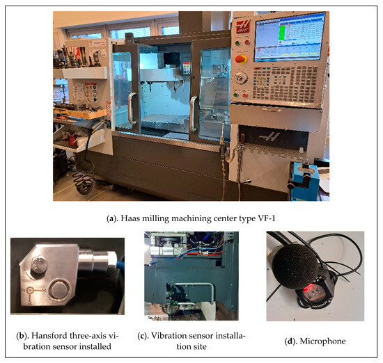
Figure 1.
Haas milling machining center type VF-1 with sensors.
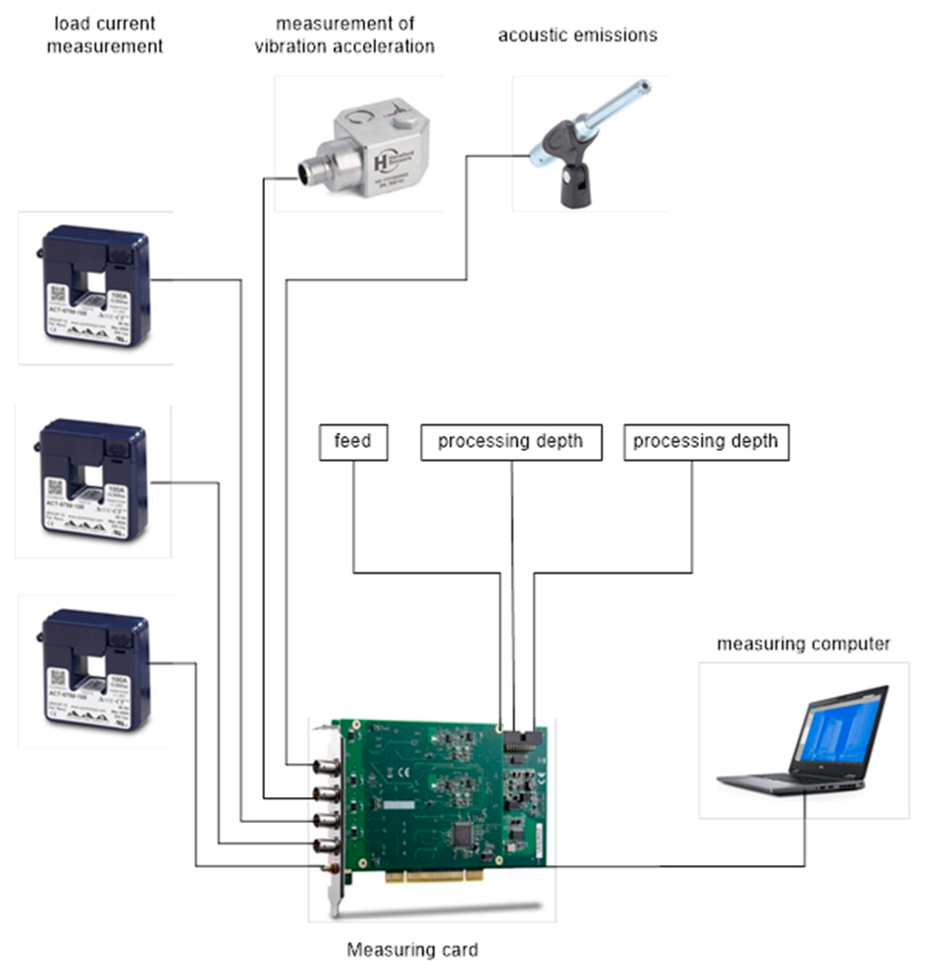
Vibration measurements were taken near the machine spindle. A three-axis Hansford sensor with a sensitivity of approximately 100 mV/g was selected. The design of the milling spindle made it impossible to install the vibration sensor directly inside the machine’s working chamber. The sensor was installed in the place closest to the spindle bearing after removing the machine covers. For this reason, it was decided to install an independent acoustic signal source inside the machine’s working chamber. A microphone with a sensitivity of approximately 50 mV/Pa was selected. An additional parameter measured was the power consumption of the milling machine from one of the phases. A current transformer with a sensitivity of approximately 10 mV/A AC was used to record from this source. The cables from the above-mentioned transducers were secured and routed to the measurement system consisting of signal conditioners, a measurement card, and a laptop with installed data visualization and recording software. The system was calibrated using calibrated reference signals. To ensure the reliability of the obtained data, the new sensors were tested on dedicated calibration stations. The entire measurement track was calibrated with standards independently before each series of measurements.
Figure 2 presents the scheme illustrating all the recording signals.

Figure 2.
Scheme illustrating all the recording signals.
In the research, the accuracy of measurements of selected physical quantities was analyzed using algorithms taking into account the current metrological properties of the measurement paths of these quantities in the full range of processing. The metrological properties of the measurement paths were determined as a result of the developed methods for the calibration of sensors and measurement paths under laboratory conditions. Data representing the cluster-zone processing in the experiments were acquired in real time. The main goal of this stage was to obtain qualitative data from measurements of electrical and non-electrical quantities.
For the experiments, 1.7225 steel samples with a hardness of 45 ± 2 HRC were utilized. Two types of cutters, namely, a TEFS-E44-CF and a TEC-A4, were employed in the research.
The study focused on the milling process, a machining technique involving the removal of successive material layers until the desired object geometry is achieved. Key parameters in the milling process encompass cutting speed, feed speed, as well as the depth and width of the cut. Optimal parameters are determined based on specialized tables provided by the tool manufacturer. The input parameters for the process are the cutting tool, material, and technological process parameters (x1—cutting speed, x2—feed speed, and x3—depth of cut). Additionally, spindle load and spindle vibrations were recorded during the tests. The following process parameters were defined: cutter Φ 6 mm (4 blades), turn-over 5300 rpm, feed speed 1270 mm/min, cutting speed approximately 100 m. During the milling process, data from the installed sensors were recorded and collected in real time.
The aim of second phase of the research was to develop advanced methods and models for analyzing industrial measurement data in order to refine the raw data into predictions that support decisions for monitoring and supervising the condition of cutting tools. Logistic regression and a gradient boosting classifier were used to develop predictive models.
3. Results and Discussion
3.1. Preliminary Analysis of the Results Obtained
An analysis of signals originating from sensors mounted on a prepared research station was conducted. The study encompassed 10 material processing samples, with a maximum of four processing layers applied to each sample. Before each processing step, a new milling tool was mounted on the machine spindle to ensure consistent measurement conditions.
The recorded signals had a sampling frequency of 10 kHz and were monitored through various channels:
- Channel A0 included signals from the Z-axis sensor, associated with the machine’s movement along the Y-axis.
- Channel A1 recorded signals from the Y-axis sensor, associated with the machine’s movement along the Z-axis.
- Channel A2 was responsible for recording signals from the X-axis sensor, associated with the machine’s movement along the X-axis.
- Channel A3 encompassed signals from a microphone with a sensitivity of 50 mV/Pa, used for monitoring the noise generated during processing.
- Channel A4 recorded signals from the spindle current transducer, providing information about the current in that area.
- Channel A5 included signals from the milling machine’s current transducer, supplying information about the current in the milling area.
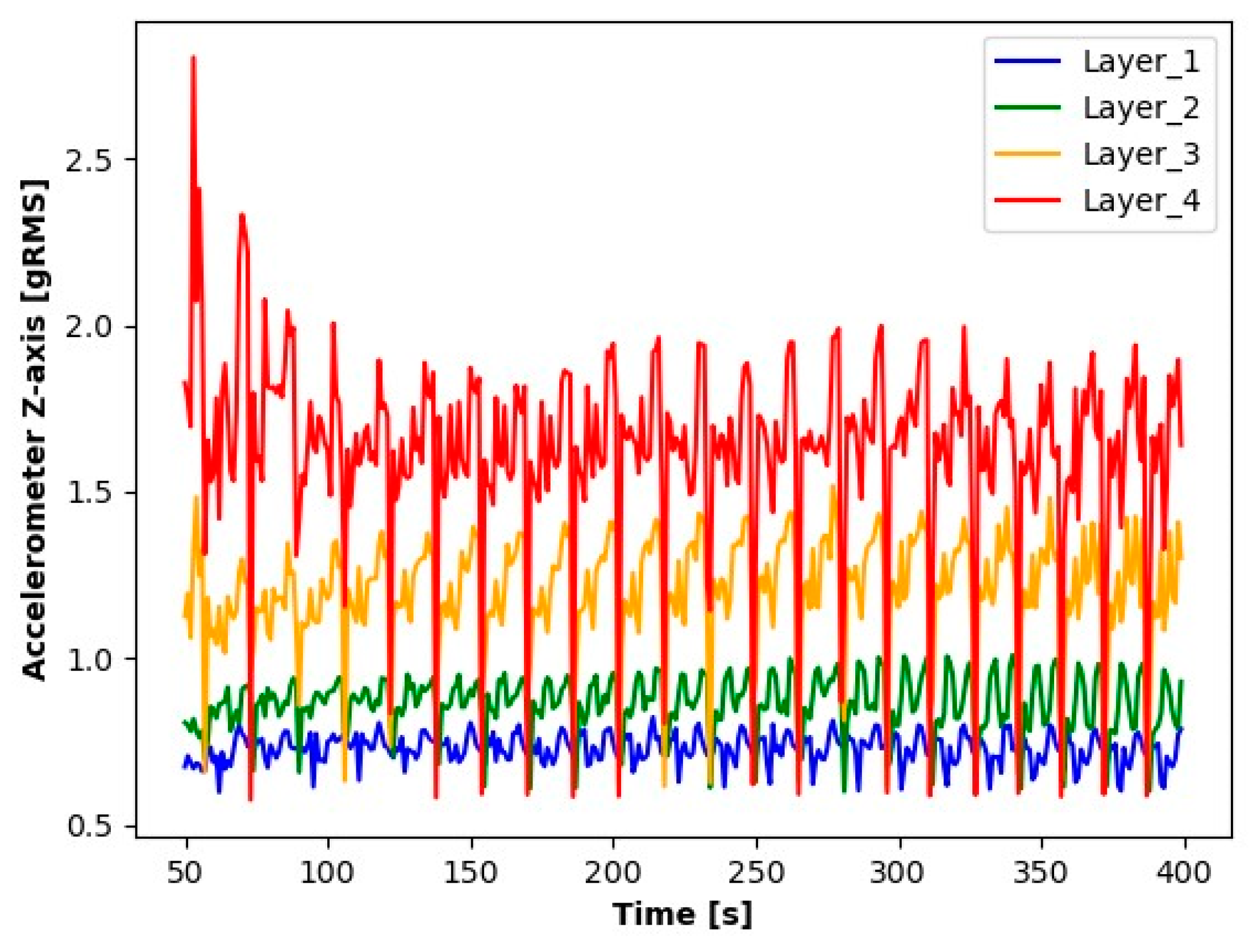
The first step in the initial analysis was signal processing. For each layer to be analyzed, the signal readings were divided into sequences containing 10.000 elements (a sequence contains a 1 s signal reading). The average values of these series were determined for the accelerometer, as were the absolute average values for microphone signals. For the current transformer, averages were determined from the absolute values of the readings. The signal processing results (averages for each second) for the first sample during seconds 50 to 400 are shown in the Figure 3, Figure 4, Figure 5, Figure 6, Figure 7 and Figure 8.

Figure 3.
Results of Z-axis accelerometer readings.
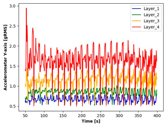
Figure 4.
Results of Y-axis accelerometer readings.
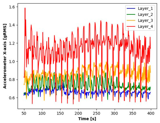
Figure 5.
Results of X-axis accelerometer readings.

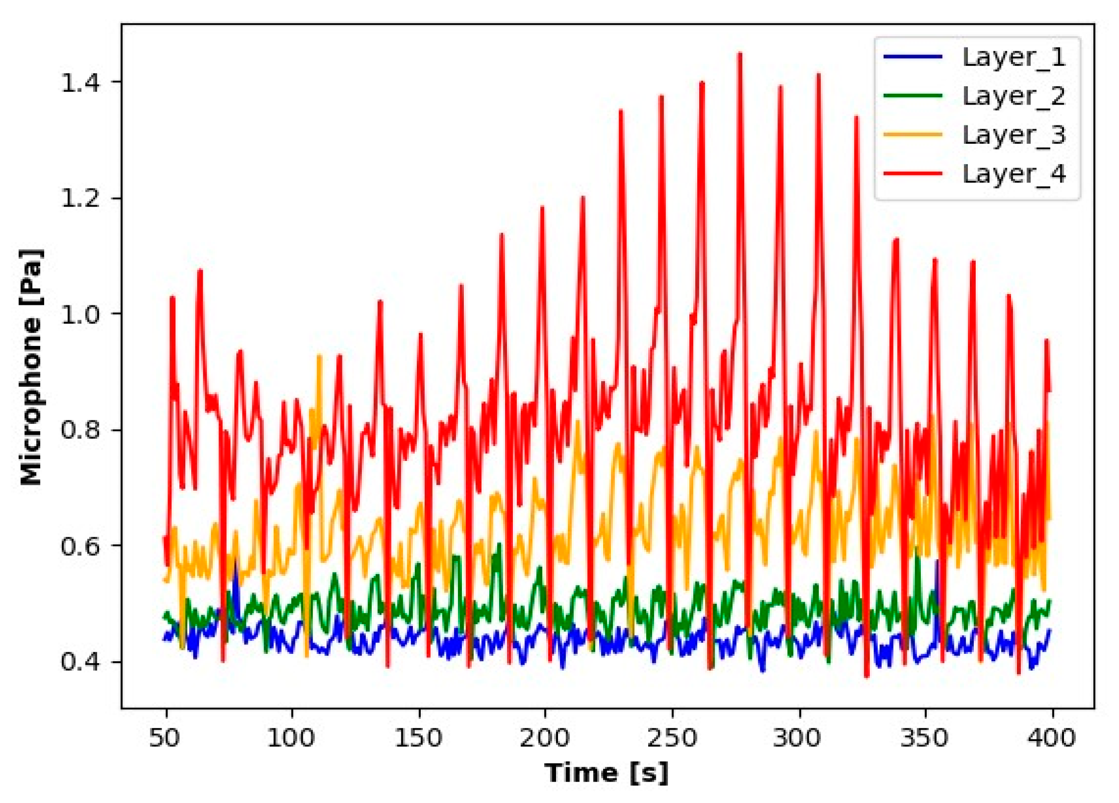
Figure 6.
Reading results for the microphone.

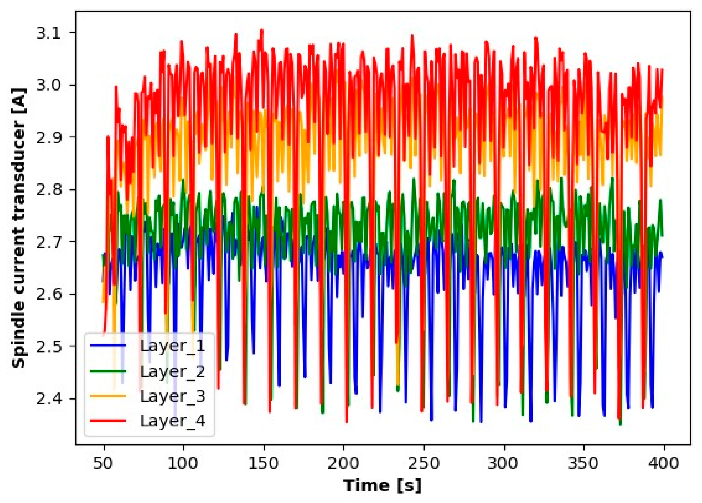
Figure 7.
Reading results for the spindle current transducer.
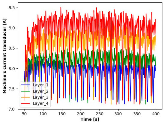
Figure 8.
Reading results for the current transducer of the milling machine.
The results presented suggest observable differences in the signal values for each layer. When analyzing the graphs, clear differences in the averages for each of the signals tested are noticeable. Particularly for Layer 1, it can be observed that the average signal values are significantly smaller compared to the other layers. An increase in the average values for the subsequent layers suggests a process of wear of the cutting tool.
The next step in the preliminary data analysis was to analyze the values of the signals obtained. The main objective of the signal analysis was to identify mechanisms that enable the recognition of the condition of the cutter from the signal readings.
Let denote the sequence of average values from one-second readings, i.e., the value of the is the average of 10,000 signals obtained from the sensor. The analyzed is the one-second sequences of averages for , is the integer part of the number. For second sequences , the mean value and the variance for every layer were determined:
Thus, the sequence is obtained, the elements of which belong to the two-dimensional space .
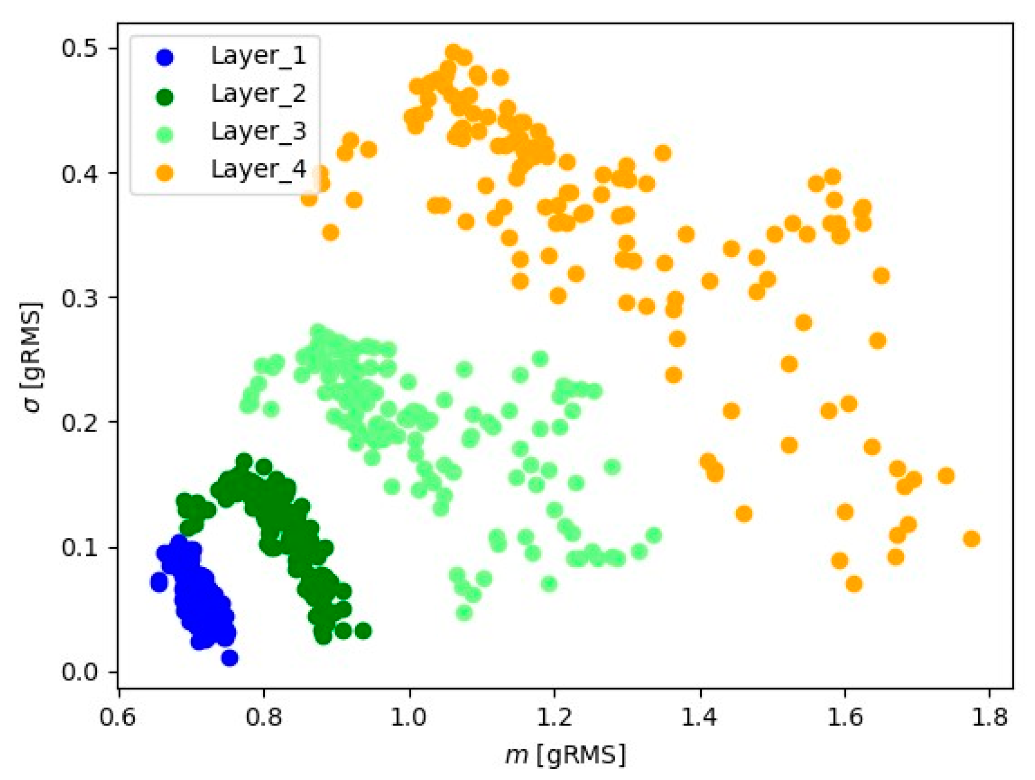
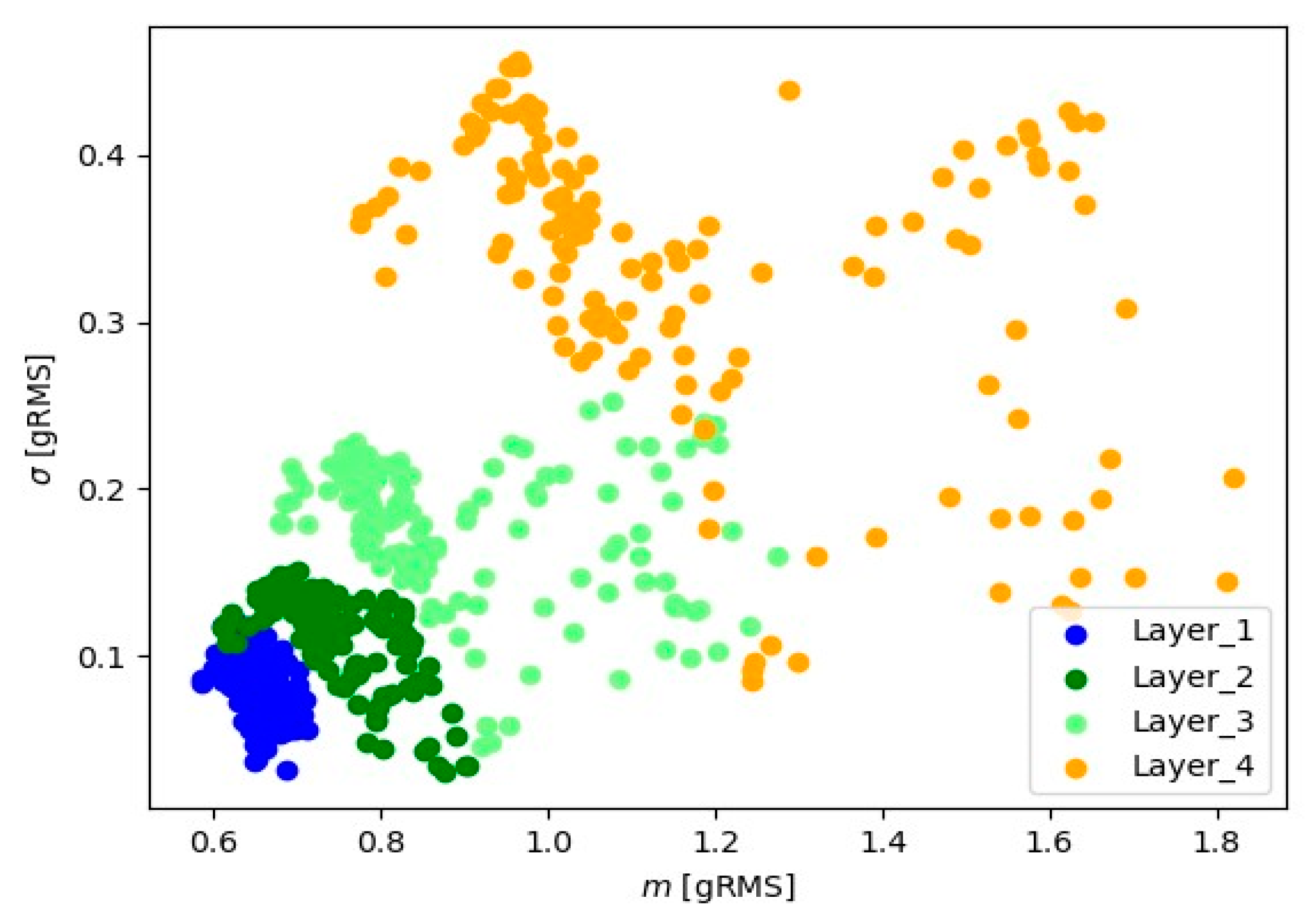
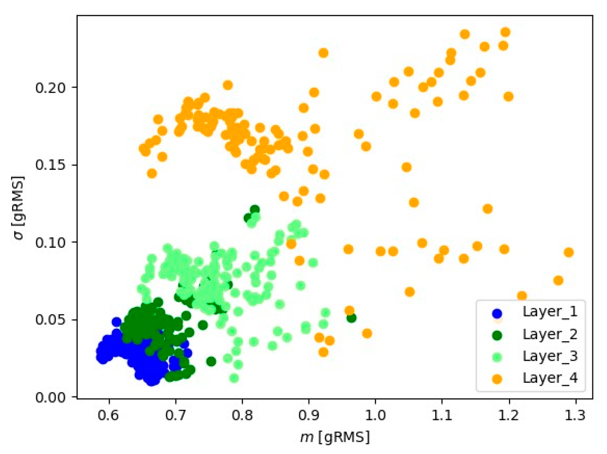
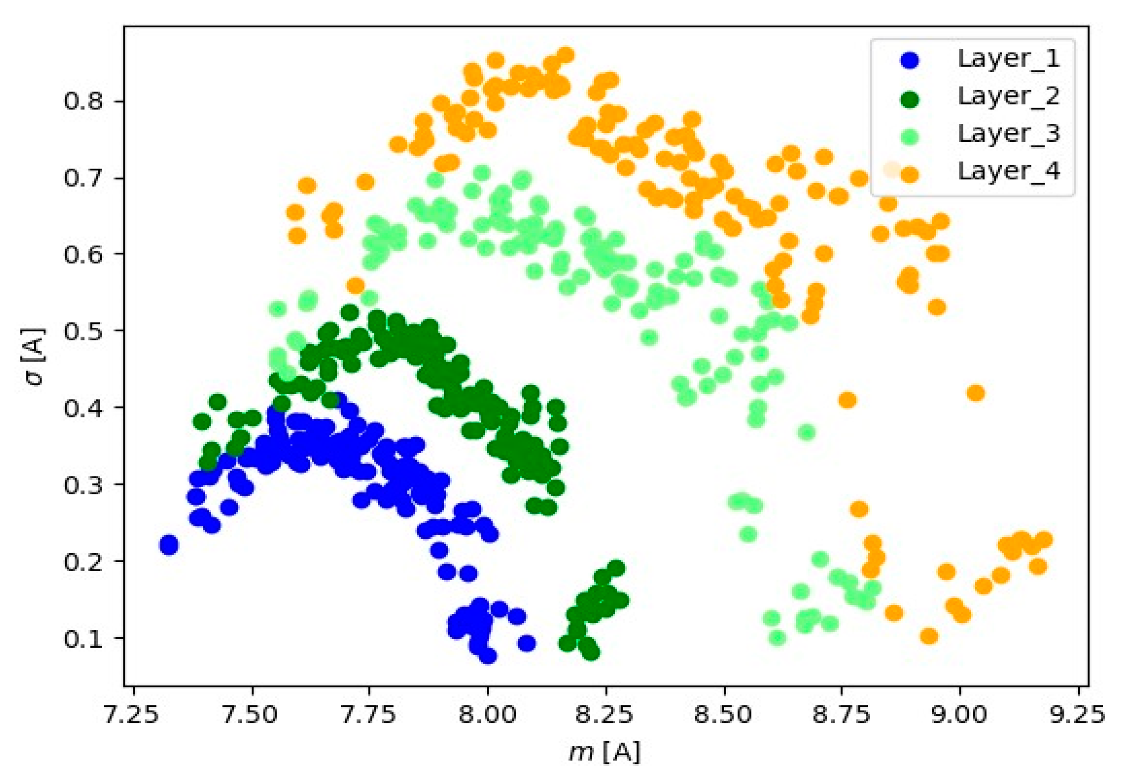
In Figure 9, Figure 10, Figure 11, Figure 12, Figure 13 and Figure 14, the obtained results for sample No. 1 are presented.

Figure 9.
Representation of 10 s signals for the Z-axis accelerometer.

Figure 10.
Representation of 10 s signals for the Y-axis accelerometer.

Figure 11.
Representation of 10 s signals for the X-axis accelerometer.
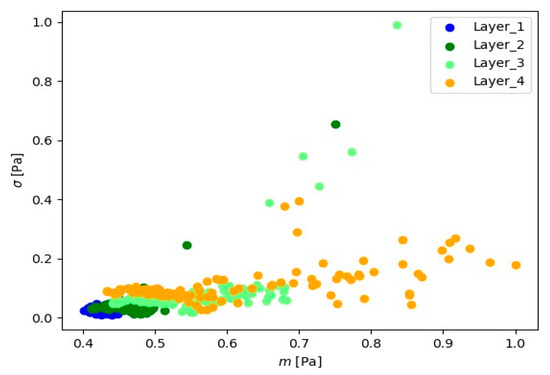
Figure 12.
Representation of 10 s microphone signals.
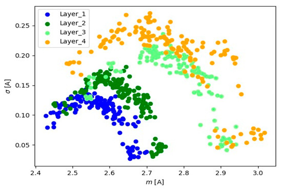
Figure 13.
Representation of 10 s signals for the spindle load current transformer.

Figure 14.
Representation of 10 s signals for the current transformer of the milling machine load.
Visual analysis using the ‘mean-standard deviation’ system provides crucial information about signal positioning for various layers. The observed distinct differences in signal position suggest the presence of well-defined groups of signal readings for each material layer. In the ‘mean-standard deviation’ system, the mean refers to the central value, and the standard deviation determines the quantity of dispersion around the mean. The observed differences in signal position across different signal layers indicate variations in signal characteristics during various stages of material processing. These signal groupings suggest the existence of distinct features and parameters for each layer, which could be linked to fluctuations in cutting tool conditions.
Table 1 presents the minimum and maximum signal values for each layer and signal type (channel).

Table 1.
Smallest and largest values of mean and standard deviation depending on layer and signal type.
From the results presented in Table 1, it is observed that as the cutter time increases, the range of basic statistics (mean and standard deviation) increases too. In Layer_1, the mean values are between 7.3230 and 8.0840, and the standard deviations range from 0.0758 to 0.4098. In Layer_2, the mean values remain between 7.3959 and 8.2794, and the standard deviations range from 0.0811 to 0.5234. In Layer_3, the mean values are between 7.5549 and 8. 8139, and the standard deviations range from 0.0995 to 0.7058. For the Layer_4 layer, the averages range from 7.5939 to 9.1788, and the standard deviations range from 0.1018 to 0.8588. It can be seen that there is variation in the values of the averages and standard deviations between the layers, which may indicate specific characteristics of the signals in each layer. Layer_4 shows the largest range of mean values and standard deviations, which may suggest greater variability in the signals of this layer. This indicates that the analyzed signals show differences specific to each layer.
The change in mean values and standard deviation is also noticeable between individual channels. For channel A0, the minimum values range from 7.3230 to 7.5939 across all layers, and the maximum values gradually increase from 8.0840 to 9.1788 from Layer_1 to Layer_4. The standard deviation shows a slight increase from 0.0758 to 0.1018 as we move through the layers. This pattern is consistent across all channels (A1 to A5), where minimum values remain relatively constant, maximum values gradually increase with layers, and the standard deviation shows minor changes.
Summarizing, the data analysis revealed consistent behavior across all channels, with the primary changes occurring between layers. This consistent trend suggests that any deviations or anomalies in the data are more likely to be specific to certain layers rather than specific channels. The main task in layer identification involves, on one hand, processing the raw signal, and on the other, constructing a classifier that could recognize the layer in the analyzed case, which is directly related to cutter wear. Since six signals were analyzed, basic statistics such as the mean value and standard deviation were determined for each signal based on 10 s readings. These statistical values were used as predictors for the classification models. This information has been supplemented in the content of the article.
3.2. Construction of the Classifier
3.2.1. Creating a Database
In the process of signal analysis, each signal was analyzed in detail by dividing it into sequences of 100,000 elements. For each of these sequences, mean values were calculated for the signals coming from both the accelerometer and the microphone. For the signals from the current transformer, mean absolute values were determined. This process made it possible to create new sequences representing the averages for the individual signal channels.
The data set contains 3738 records. Table 2 presents the distribution of the number of cases for each layer in this data set.
Table 2.
Number of cases in the data set for each layer.
The differences in the number of cases between layers reflect the variation in samples from different stages of the process, which is an important aspect in terms of analyzing the signals and understanding their characteristics depending on the material layer.
In order to effectively develop a classifier to identify the layer of material being processed, the data set was divided into a learning set, representing 80% of the cases, and a test set, comprising 20% of the cases. The test set consists of 748 instances.
Let denotes the data set . Elements of the sequence are the values of basic statistics such as the mean value and standard deviation determined on the basis of 10-s readings from the sensors. The elements of the vectors belong to the four classes and are predictors for classification models. The following methods were used to construct the classifier for identifying the layer of processed material:
- Logistic regression;
- Gradient boosting classifier.
These advanced classification models are designed to effectively recognize layers of processed material based on signal analysis. Their effectiveness will be tested on the test set, which will allow for assessing the effectiveness of the classifier. This approach allows one to develop an understanding of the machining process and to improve the precision of identifying material layers, which is a key element of optimizing production processes.
3.2.2. Logistic Regression
Let be the probabilistic space, and . Logistic regression describes the distribution of the probability of realizing the random variable based on the realization of the independent variables [29,30]. To apply logistic regression for each of the classes , modify the training set , where
and the value
means (odds).
In logistic regression, we analyze the linear dependence of the logarithm of the odds based on the realization :
where is a random variable with a normal distribution and . From Formula (3), we have:
For each class , we solve the task
where the likelihood function is given by:
To estimate the structural parameters of for the class, task (5) is replaced by an auxiliary task:
where
When the predictors are collinear, then ELASTICNET regularization [31,32] is additionally used. The parameters of linear regression in model (7) are determined by solving the problem:
where , , and means the penalty given by the formula:
For each class, the parameters , were estimated. For the realization of independent variables , the probability of belonging to the th class was assessed as follows:
The results of the analysis of the use of logistic regression for the test set were presented using a confusion matrix and the overall accuracy of the classifier (Table 3). The overall accuracy of the model is 90.78%. The classifier successfully identifies Layer 1, achieving 254 correct predictions and only seven errors. However, as the number of layers increases, errors increase, especially for Layer 2 and Layer 3, which may require further optimization of the model. It is worth paying attention to cases where errors occur, which may suggest difficulties in distinguishing between certain classes.
Table 3.
Confusion matrix for logistic regression.
Additionally, characteristics were estimated for each class (Table 4). The analysis of the logistic regression classifier’s recognition characteristics demonstrates the effectiveness of the model in classifying individual layers. High values for sensitivity (Recall) indicate that the model effectively identifies positive cases in all layers. Specificity is also high, indicating effective detection of negative cases. The Precision (positive predictive values—Pos Pred Value) exhibits variability, with the highest being seen in Layer 1 and the lowest in Layer 4. Furthermore, the negative predictive values (Neg Pred Value) generally remain high, particularly for Layer 4. Precision and Recall demonstrate satisfactory outcomes, although there is some variation in F1 score among the classes. Prevalence denotes the distribution of categories in the training set, with Layer 1 and Layer 2 being predominant. Balanced Accuracy persists at a high level across all layers.
Table 4.
Classifier recognition characteristic values for each class for logistic regression.
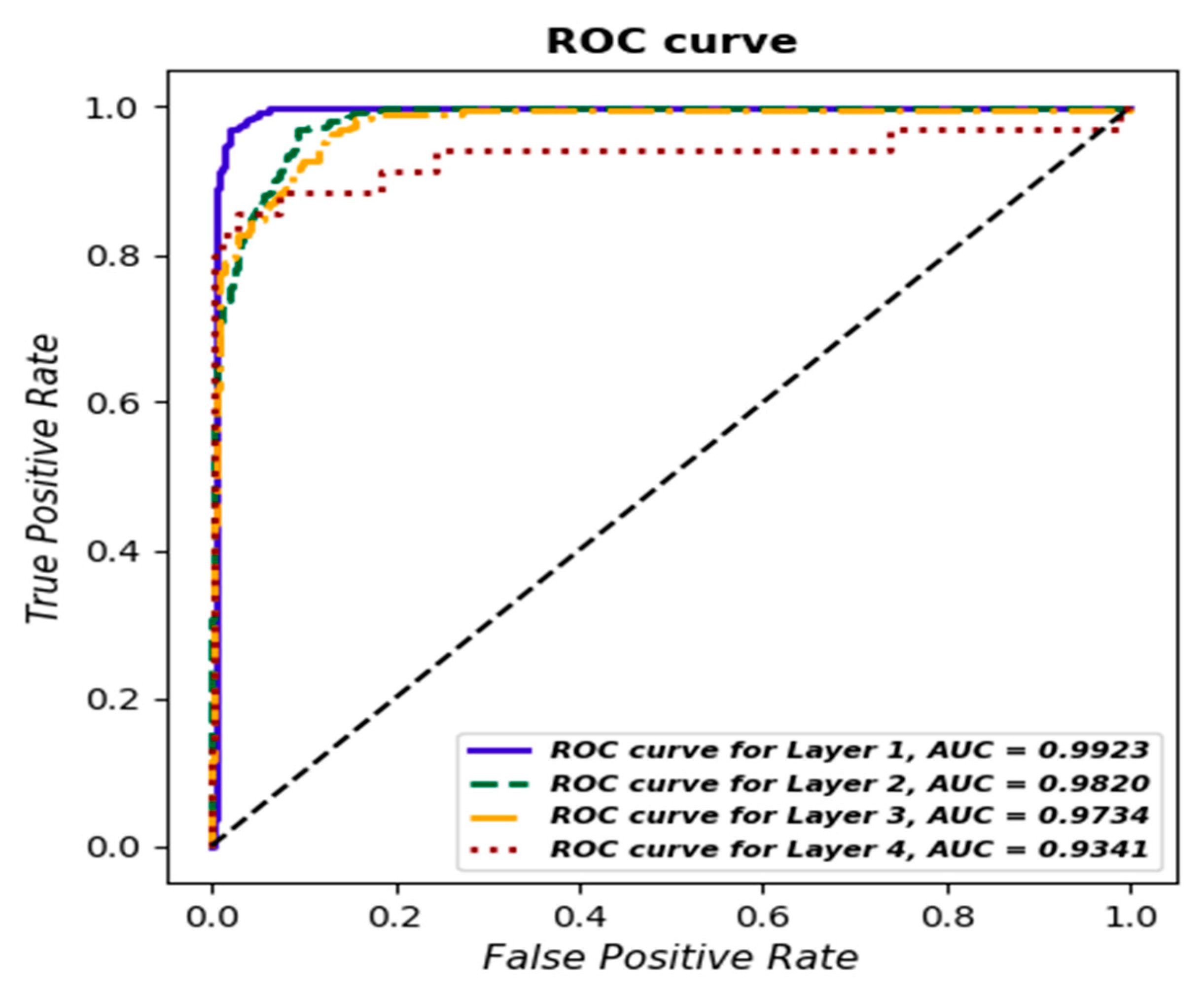
Additionally, a ROC curve was determined for each class, and AUC values were estimated (Figure 15), with the best results obtained for Layer 1—AUC = 0.9923.
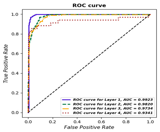
Figure 15.
ROC curve for each layer based on logistic regression.
ROC curves and AUC values confirm the overall quality of the classifier in distinguishing between classes. This analysis is an important tool for assessing the effectiveness of the model and indicates areas that may require further optimization [33].
3.2.3. Gradient Boosting Classifier
Boosting is one of the learning methods. It was originally implemented for the classification problem. The idea of the boosting method consists in combination with the ‘weak’ classifiers set to produce the ‘powerful’ classifier [34,35].
Thus, the gradient boosting classifier [31] relies on the definition of the sequence of trees , where the classification-boosted model based on trees is created as follows:
To identify the layer of processed material, we determine the boosted model based on data set , where but for . The boosting trees (11) are determined by applying a forward stagewise procedure. The classification tree is forced to concentrate on observations that are misclassified by boosted model . In every step , the tree is defined as follows:
where denotes a set of separable regions:
From the above the sequence, identifies the parameters of the th classification tree. For the th step (), the parameters of tree (12) were estimated by the solution of the task:
where denotes the loss function, and , . In this case, the K-class exponential loss function was used [36].
The results of the analysis of the application of the gradient boosting classifier for the test set are presented in the confusion matrix (Table 5).
Table 5.
Confusion matrix for gradient boosting classifier.
The values in each cell represent the number of cases assigned to the class. For example, the number 261 in the first row and first column means that for true Layer 1 instances, the classifier also correctly predicted Layer 1 in 261 instances.
The overall accuracy of the classifier on the test set is 97.46%, which means that almost 98% of the instances were classified correctly. The classifier seems to be effective in discriminating between different layers, especially for Layer 1 and Layer 2, where it achieves very high accuracy. It is worth noting that the lack of errors in Layer 1 may suggest that this class is relatively easy for the classifier to recognize.
However, it is also important to note individual error cases, such as the seven cases in which Layer 3 was misclassified as Layer 4. Analysis of these cases may be important to understand the specifics of the classifier’s errors and potential areas for further optimization.
The obtained results suggest that the gradient boosting classifier performs well in classifying the different layers, offering high overall accuracy, but it is worth analyzing the error cases in detail for possible model improvement.
Additionally, characteristics were estimated for each class, and their values are presented in Table 6.
Table 6.
Values of the classifier’s recognition characteristics for each class.
Analysis of the results for the gradient boosting classifier reveals the classifier’s excellent ability to effectively identify individual classes. The sensitivity (Recall) for each of the layers (Layer 1–4) remains at an impressive level of over 95%, demonstrating the classifier’s ability to effectively identify instances of a particular class from among all actual instances of that class.
Specificity for most layers also remains at a very high level, demonstrating the ability of the classifier to correctly detect cases that do not belong to a given class among all cases that do not belong to that class.
The Precision (Positive Pred Value) for most of the strata approach 1, indicating the effective detection of true positive cases. Neg Pred Value values also remain high, indicating effective elimination of false positive cases.
Comparing the layers, it can be seen that Recall, Specificity, and Precision are highest for Layer 1, suggesting that for this class, the classifier achieves the highest performance. Layer 3 achieves the lowest Precision, but it still maintains a satisfactory level.
Balanced Accuracy for each layer remains very high, confirming the overall effectiveness of the classifier in the context of the balanced classification problem.
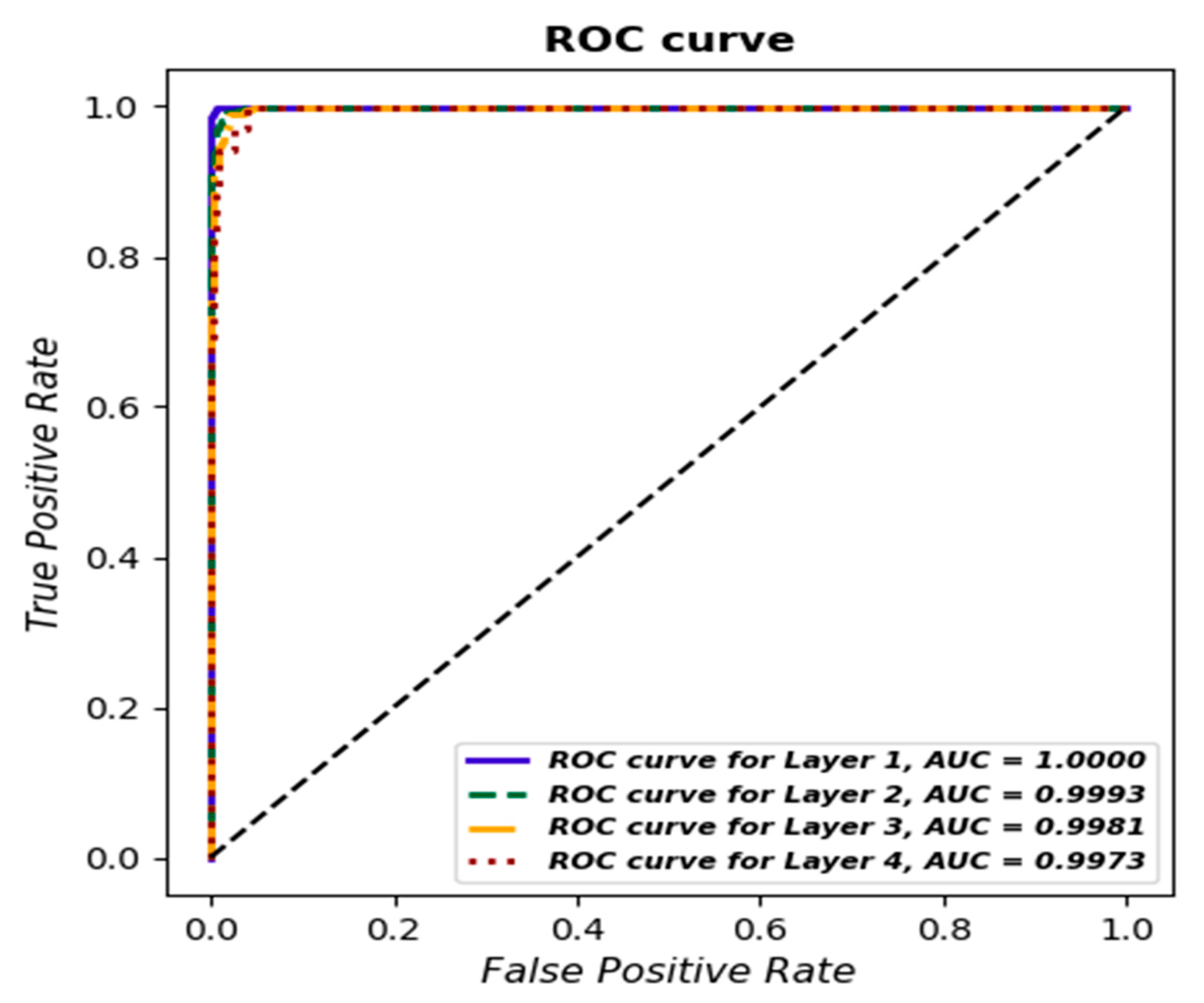
Additionally, as for the previous model, a ROC curve was determined for each class, and the AUC value was estimated (Figure 16).
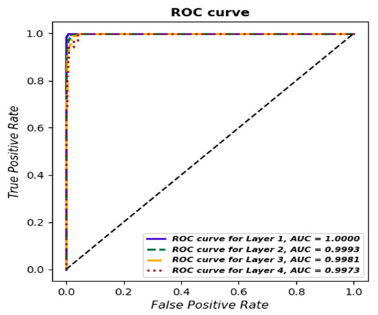
Figure 16.
ROC curve for each layer based on gradient boosting classifier.
Comparing the recognition of layers, it can be seen that the gradient boosting classifier (97.46%) has a better overall accuracy on the validation (test) set than the logistic regression (90.78%). Precision (Positive Pred Value—the proportion of correctly recognized positive cases among positively classified cases) and Recall (sensitivity—the proportion of positively recognized positive cases among positive cases) are responsible for the accuracy of recognizing individual layers (as positive cases).
Moreover, comparing the Precision values, it can be seen that regardless of the layer, better results were obtained for gradient boosting classifier. A new cutter was used for Layer 1, and the cases for Layer 1 were accurately recognized by the gradient boosting classifier (i.e., Precision = 1). For logistic regression, Precision is 0.9732. For the remaining layers, the Precision in the gradient boosting classifier is at least 0.8, whereas for logistic regression, it is less than 0.66 for Layer 4.
The recall for the gradient boosting classifier is at least 0.95 regardless of the strata, whereas for logistic regression, it is below 0.95. When analyzing the area under the curve, it can be observed that for the gradient boosting classifier, it is above 0.99 regardless of the layer, whereas for logistic regression, it is above 0.99 only for Layer 1.
Therefore, by analyzing the above layer detection characteristics (which are equivalent to cutter wear), the gradient boosting classifier identifies the cutter condition quite accurately.
4. Conclusions
The proper identification and management of tool wear in milling processes is extremely important to ensure the integrity and quality of machined objects while minimizing economic losses. This commitment to quality control and efficiency aligns perfectly with the overall concept of sustainable development—a paradigm that seeks to harmonize economic progress with environmental responsibility and social equality.
In the context of sustainable development, recognizing and addressing tool wear not only contributes to the economic sustainability of production processes but also aligns with environmental conservation goals. By optimizing the use of tools and extending their lifespan through the precise identification of wear, it possible to reduce the demand for new tools, resulting in lower consumption of raw materials and energy needed for their production.
Literature reviews have pointed out the need for developing innovative approaches and techniques that can effectively handle the asymmetry in data distribution. Furthermore, the application of alternative machine-learning methods to develop highly accurate predictive models is recommended. In this context, the main goal of the article was to develop predictive models enabling the identification of changes in the tool condition during milling. The research was conducted on various material samples subjected to different machining layers, providing a significant perspective in the analysis. The research results:
- Confirm the effectiveness of the applied predictive models, especially the gradient boosting classifier, which achieved high accuracy at 97.46%. The analysis of ROC curves and AUC values further confirmed the high quality of the classifiers, emphasizing their ability to precisely identify different material layers. It is worth noting that the analysis of sensor signals was comprehensive, covering various machine monitoring channels, which additionally enhances the credibility of the obtained results;
- Not only confirm the importance of monitoring tools in the milling process but also introduce innovative approaches that can significantly improve the effectiveness of this process in production conditions;
- Confirm that the implementation of the proposed models could play a crucial role in diminishing the occurrence of nonconforming products attributed to the condition of the cutting tool. These considerations are poised to curtail the consumption of raw materials, minimize production waste, and consequently alleviate the environmental impact of the company. This aligns seamlessly with the principles of sustainable production.
The results obtained in this study are better than those previously conducted in the analyzed area. For example, in [17], the use of singular spectrum analysis and a neural network resulted in a lower accuracy of 67.4%. However, in publication [19], an accuracy of 98.9% was achieved using an approach integrating force, acoustic emission, and vibration signals, which is similar to the comprehensive analysis of the sensor signal in the present study. Moreover, the work in [22] achieved a remarkable accuracy of 99.67% using a convolutional neural network focusing on cutting force signals. What is more, slightly worse results are presented compared to the results obtained in this study in the works in [26,28], with an accuracy of 92.4% and 97.3%, respectively. In addition, slightly worse results in the accuracy of the model were presented in the works in [37,38,39] using, e.g., GBC. The obtained models achieved an accuracy of 80%, 97%, and 92.98%, respectively.
The research on tool wear management in milling processes, though offering significant insights for quality control, economic efficiency, and alignment with sustainable development principles, presents several inherent limitations:
- The heavy reliance on machine-learning models, particularly methods like gradient boosting classifiers, poses its own set of challenges. Though these models have shown high accuracy, their performance is contingent on the availability of substantial and quality data. In situations with limited or noisy data, their applicability and effectiveness could be compromised.
- The research’s focus on specific materials and machining layers also raises questions about the generalizability of the findings. The models developed might require additional adjustments to be applicable to different materials or layers, limiting their immediate transferability to other manufacturing contexts.
- Despite being comprehensive and covering various machine monitoring channels, it is possible that not all aspects of tool wear are fully captured through these channels. There might be facets of tool wear or conditions that remain undetected, which could affect the overall accuracy and reliability of the predictive models.
- The practical implementation of these models in real-world production settings is another area of concern. Integrating these advanced systems with existing manufacturing processes, training personnel, and ensuring consistent performance under varying operational conditions could pose significant challenges, especially in less technologically advanced facilities.
5. Directions of Future Research
Future research in this area should focus on several key areas to understand and optimize machining processes and tool wear. The first step is to experiment with different machining tools. Conducting tests using tools of various types, sizes, and materials will help us to understand how changing the tool affects the results. Equally important is the optimization of process parameters, such as rotational speed, feed rate, or cutting depth, to see how these changes affect the quality of machining and tool wear.
Next, research should focus on testing the different materials being machined. Conducting a series of experiments on various materials will allow for a comparison of how tool wear and machining quality change depending on the material properties.
A key element of the research is the analysis of tool wear. Regular measurements of the surface roughness of the machined surface can provide information about the degree of tool wear.
Moreover, considering that data analysis indicates consistent behavior across different channels, with major changes occurring between layers, future research should focus on a detailed examination of those layers where the greatest changes were observed. Analysis of individual channels can also help identify specific channels that exhibit different behavior.
Additionally, the use of data analysis and modeling of the machining process can bring new perspectives. Creating additional models by applying different machine-learning methods to analyze large data sets from experiments can help identify patterns and relationships that are not obvious with traditional analysis methods.
Author Contributions
Conceptualization, E.K. and K.A.; methodology, E.K., K.A., J.S. and S.P.; software, E.K.; validation, E.K. and K.A.; formal analysis, E.K. and K.A.; investigation, E.K., K.A. and S.P.; resources, K.A., J.S. and S.P.; data curation, K.A., J.S. and S.P.; original draft preparation, E.K. and K.A.; writing—review and editing, E.K., K.A. and J.S.; visualization, E.K.; supervision, K.A.; project administration, K.A. funding acquisition, K.A. All authors have read and agreed to the published version of the manuscript.
Funding
The research leading to these results has received funding from the commissioned task entitled “VIA CARPATIA Universities of Technology Network named after the President of the Republic of Poland Lech Kaczyński”, contract number MEiN/2022/DPI/2575, action entitled “In the neighborhood—inter-university research internships and study visits.”. This work was prepared within the project “Innovative measurement technologies supported by digital data processing algorithms for improved processes and products”, contract number PM/SP/0063/2021/1, financed by the Ministry of Education and Science (Poland) as a part of the Polish Metrology Program.
Data Availability Statement
Data supporting this study are included within the article.
Conflicts of Interest
The authors declare no conflicts of interest.
References
- Borucka, A.; Kozłowski, E.; Parczewski, R.; Antosz, K.; Gil, L.; Pieniak, D. Supply Sequence Modelling Using Hidden Markov Models. Appl. Sci. 2023, 13, 231. [Google Scholar] [CrossRef]
- Sayyad, S.; Kumar, S.; Bongale, A.; Kamat, P.; Patil, S.; Kotecha, K. Data-driven remaining useful life estimation for milling process: Sensors, algorithms, datasets, and fu-ture directions. IEEE Access 2021, 9, 110255–110286. [Google Scholar] [CrossRef]
- Pimenov, D.Y.; Gupta, M.K.; da Silva, L.R.; Kiran, M.; Khanna, N.; Krolczyk, G.M. Application of measurement systems in tool condition monitoring of Milling: A review of measurement science approach. Measurement 2022, 199, 111503. [Google Scholar] [CrossRef]
- Kozłowski, E.; Antosz, K.; Mazurkiewicz, D.; Sęp, J.; Żabiński, T. Integrating advanced measurement and signal processing for reliability decision-making. Eksploat. I Niezawodn.—Maint. Reliab. 2021, 23, 777–787. [Google Scholar] [CrossRef]
- Antosz, K.; Mazurkiewicz, D.; Kozłowski, E.; Sęp, J.; Żabiński, T. Machining Process Time Series Data Analysis with a Decision Support Tool. In Innovations in Mechanical Engineering, Lecture Notes in Mechanical Engineering; Machado, J., Soares, F., Trojanowska, J., Ottaviano, E., Eds.; Springer: Berlin/Heidelberg, Germany, 2022; pp. 14–27. [Google Scholar]
- Li, X.; Yue, C.; Liu, X.; Zhou, J.; Wang, L. ACWGAN-GP for milling tool breakage monitoring with imbalanced data. Robot. Comput.–Integr. Manuf. 2024, 85, 102624. [Google Scholar] [CrossRef]
- Lu, X.; Jia, Z.; Wang, H.; Feng, Y.; Liang, S.Y. The effect of cutting parameters on micro-hardness and the prediction of Vickers hardness based on a response surface method-ology for micro-milling Inconel 718. Meas. J. Int. Meas. Confed. 2019, 140, 56–62. [Google Scholar] [CrossRef]
- Feng, Y.; Hung, T.P.; Lu, Y.T.; Lin, Y.F.; Hsu, F.C.; Lin, C.F.; Lu, Y.C.; Lu, X.; Liang, S.Y. Inverse analysis of inconel 718 laser-assisted milling to achieve machined surface roughness. Int. J. Precis. Eng. Manuf. 2018, 19, 1611–1618. [Google Scholar] [CrossRef]
- Lu, X.; Wang, X.; Sun, J.; Zhang, H.; Feng, Y. The influence factors and prediction of curve surface roughness in micro-milling nickel based superalloy. In Proceedings of the ASME 2018 13th International Manufacturing Science and Engineering Conference, MSEC 2018, College Station, TX, USA, 18–22 June 2018; American Society of Mechanical Engineers: New York, NY, USA, 2018; p. V004T03A010. [Google Scholar] [CrossRef]
- Feng, Y.; Hung, T.P.; Lu, Y.T.; Lin, Y.F.; Hsu, F.C.; Lin, C.F.; Lu, Y.C.; Lu, X.; Liang, S.Y. In-verse analysis of the cutting force in laser-assisted milling on Inconel 718. Int. J. Adv. Manuf. Technol. 2018, 96, 905–914. [Google Scholar] [CrossRef]
- Zhou, Y.; Sun, W.; Ye, C.; Peng, B.; Fang, X.; Lin, C.; Wang, G.; Kumar, A.; Sun, W. Time-frequency Representation -enhanced Transfer Learning for Tool Condition Monitoring during milling of Inconel 718. Eksploat. I Niezawodn.—Maint. Reliab. 2023, 25, 165926. [Google Scholar] [CrossRef]
- Dutta, S.; Pal, S.K.; Mukhopadhyay, S.; Sen, R. Application of digital image processing in tool condition monitoring: A review. CIRP J. Manuf. Sci. Technol. 2013, 6, 212–232. [Google Scholar] [CrossRef]
- Kozłowski, E.; Mazurkiewicz, D.; Żabiński, T.; Prucnal, S.; Sęp, J. Machining sensor data management for operation-level predictive model. Expert. Syst. Appl. 2020, 159, 113600. [Google Scholar] [CrossRef]
- Tran, M.Q.; Doan, H.P.; Vu, V.Q.; Vu, L.T. Machine Learning and IoT-Based Approach for Tool Condition Monitoring: A Review and Future Prospects. Measurement 2022, 207, 112351. [Google Scholar] [CrossRef]
- Isavand, J.; Kasaei, A.; Peplow, A.; Wang, X.; Yan, J. A Reduced-Order Machine-Learning-Based Method for Fault Recognition in Tool Condition Monitoring. Measurement 2023, 224, 113906. [Google Scholar] [CrossRef]
- Salgado, D.R.; Alonso, F.J. Tool Wear Detection in Turning Operations Using Singular Spectrum Analysis. J. Mater. Process. Technol. 2006, 171, 451–458. [Google Scholar] [CrossRef]
- Kilundu, B.; Dehombreux, P.; Chiementin, X. Tool Wear Monitoring by Machine Learning Techniques and Singular Spectrum Analysis. Mech. Syst. Sig. Process. 2011, 25, 400–415. [Google Scholar] [CrossRef]
- He, M.; He, D. A New Hybrid Deep Signal Processing Approach for Bearing Fault Diagnosis Using Vibration Signals. Neurocomputing 2020, 396, 542–555. [Google Scholar] [CrossRef]
- Segreto, T.; Simeone, A.; Teti, R. Multiple Sensor Monitoring in Nickel Alloy Turning for Tool Wear Assessment via Sensor Fusion. Procedia CIRP 2013, 12, 85–90. [Google Scholar] [CrossRef]
- Seemuang, N.; McLeay, T.; Slatter, T. Using Spindle Noise to Monitor Tool Wear in a Turning Process. Int. J. Adv. Manuf. Technol. 2016, 86, 2781–2790. [Google Scholar] [CrossRef]
- Liu, M.-K.; Tseng, Y.-H.; Tran, M.-Q. Tool Wear Monitoring and Prediction Based on Sound Signal. Int. J. Adv. Manuf. Technol. 2019, 103, 3361–3373. [Google Scholar] [CrossRef]
- Tran, M.Q.; Liu, M.K.; Tran, Q.V. Milling Chatter Detection Using Scalogram and Deep Convolutional Neural Network. Int. J. Adv. Manuf. Technol. 2020, 107, 1505–1516. [Google Scholar] [CrossRef]
- Kothuru, A.; Nooka, S.P.; Liu, R. Application of Audible Sound Signals for Tool Wear Monitoring Using Machine Learning Techniques in End Milling. Int. J. Adv. Manuf. Technol. 2018, 95, 3797–3808. [Google Scholar] [CrossRef]
- Zhang, C.; Yao, X.; Zhang, J.; Jin, H. Tool Condition Monitoring and Remaining Useful Life Prognostic Based on a Wireless Sensor in Dry Milling Operations. Sensors 2016, 16, 795. [Google Scholar] [CrossRef] [PubMed]
- Lu, M.-C.; Wan, B.-S. Study of High-Frequency Sound Signals for Tool Wear Monitoring in Micromilling. Int. J. Adv. Manuf. Technol. 2013, 66, 1785–1792. [Google Scholar] [CrossRef]
- Schueller, A.; Saldana, C. Generalizability Analysis of Tool Condition Monitoring Ensemble Machine Learning Models. J. Manuf. Process. 2022, 84, 1064–1075. [Google Scholar] [CrossRef]
- Soori, M.; Arezoo, B.; Dastres, R. Machine learning and artificial intelligence in CNC machine tools, A review. Sustain. Manuf. Serv. Econ. 2023, 2, 100009. [Google Scholar] [CrossRef]
- He, J.; Sun, Y.; Gao, H.; Guo, L.; Cao, A.; Chen, T. On-line milling tool wear monitoring under practical machining conditions. Measurement 2023, 222, 113621. [Google Scholar] [CrossRef]
- Xin, Y.; Xiaogang, S. Linear Regression Analysis; World Scientific Publishing Company: Singapore, 2009. [Google Scholar]
- Zou, H.; Hastie, T. Regularization and Variable Selection via the Elastic Net. J. R. Stat. Soc. Ser. B Stat. Methodol. 2005, 67, 301–320. [Google Scholar] [CrossRef]
- Tibshirani, R. Regression Shrinkage and Selection via the Lasso. J. R. Stat. Soc. Ser. B 1994, 58, 267–288. [Google Scholar] [CrossRef]
- Friedman, J.; Hastie, T.; Tibshirani, R. Regularization Paths for Generalized Linear Models via Coordinate Descent. J. Stat. Softw. 2010, 33, 1–22. [Google Scholar] [CrossRef]
- Fawcett, T. An Introduction to ROC Analysis. Pattern Recognit. Lett. 2006, 27, 861–874. [Google Scholar] [CrossRef]
- Hand, D.J.; Till, R.J. A Simple Generalization of the Area Under the ROC Curve for Multiple Class Classification Problems. Mach. Learn. 2001, 45, 171–186. [Google Scholar] [CrossRef]
- Hastie, T.; Tibshirani, R.; Friedman, J. The Elements of Statistical Learning; Springer Inc.: New York, NY, USA, 2009. [Google Scholar]
- James, G.; Witten, D.; Hastie, T.; Tibshirani, R. An Introduction to Statistical Learning; Springer: Berlin/Heidelberg, Germany, 2013. [Google Scholar]
- Li, G.; Wang, Y.; He, J.; Hao, Q.; Yang, H.; Wei, J. Tool wear state recognition based on gradient boosting decision tree and hybrid classification RBM. Int. J. Adv. Manuf. Technol. 2020, 109, 2417–2428. [Google Scholar] [CrossRef]
- Alajmi, M.S.; Almeshal, A.M. Predicting the Tool Wear of a Drilling Process Using Novel Machine Learning XGBoost-SDA. Materials 2020, 13, 4952. [Google Scholar] [CrossRef] [PubMed]
- Riego, V.; Castejón-Limas, M.; Sánchez-González, L.; Fernández-Robles, L.; Pérez, H.; Díez-González, J.; Guerrero-Higueras, Á.M. Strong classification system for wear identification on milling processes using computer vision and ensemble learning. Neurocomputing 2021, 423, 643–654. [Google Scholar] [CrossRef]


Disclaimer/Publisher’s Note: The statements, opinions and data contained in all publications are solely those of the individual author(s) and contributor(s) and not of MDPI and/or the editor(s). MDPI and/or the editor(s) disclaim responsibility for any injury to people or property resulting from any ideas, methods, instructions or products referred to in the content. |
© 2023 by the authors. Licensee MDPI, Basel, Switzerland. This article is an open access article distributed under the terms and conditions of the Creative Commons Attribution (CC BY) license (https://creativecommons.org/licenses/by/4.0/).