Article

SVD-SLAM: Stereo Visual SLAM Algorithm Based on Dynamic Feature Filtering for Autonomous Driving

1
School of Automobile and Traffic Engineering, Wuhan University of Science and Technology, Wuhan 430065, China
2
Tsinghua University Suzhou Automotive Research Institute, Tsinghua University, Suzhou 215000, China
*
Author to whom correspondence should be addressed.
Electronics 2023, 12(8), 1883; https://doi.org/10.3390/electronics12081883
Submission received: 25 February 2023 / Revised: 7 April 2023 / Accepted: 15 April 2023 / Published: 17 April 2023
(This article belongs to the Section Artificial Intelligence)

Abstract

:
The conventional Simultaneous Localization and Mapping (SLAM) algorithm assumes a static world, which is easily influenced by dynamic elements of the surrounding environment. For high-precision localization in dynamic scenes, a dynamic SLAM algorithm combining instance segmentation and dynamic feature point filtering is proposed to address this issue. Initially, YOLACT-dyna, a one-stage instance segmentation network, was developed in order to perform instance segmentation on the input image, eliminate potential moving objects in the scene, and estimate the camera pose roughly. Second, based on the camera pose and polar constraint, the motion probability of each possible moving object was computed. Finally, the moving feature points were filtered out, and the static feature points were used to calculate the pose. The experimental results reveal that this algorithm’s recall rate in the dynamic regional KITTI dataset was 94.5% in public datasets. Accuracy is enhanced in environments with dynamic object location. At the same time, it can guarantee the positioning accuracy of a static scene, effectively enhancing the visual SLAM system’s position precision and robustness in a dynamic environment. It can meet the requirements of the automatic driving system’s real-time operation.

1. Introduction

SLAM technology has achieved success and is widely employed in autonomous driving, augmented reality, robotics, and surveying and mapping, among other fields [1,2,3]. Smith [4] et al. first introduced the concept of SLAM, which is a method for determining the current pose of a robot without knowing its environment and motion. Over the next three decades, the SLAM concept attracted the attention of researchers and began to develop rapidly. In particular, vision-based SLAM methods have developed rapidly in recent years and now dominate robot autonomy technology [5]. Several classic SLAM algorithms, such as PTAM [6], DS-SLAM [7], ORB-SLAM [8,9,10], and Vins-mono [11], have been proposed.
The majority of conventional visual SLAM algorithms are founded on the static world assumption, which holds that all objects in the environment are immobile. Consequently, the performance of the system will be impacted as the number of moving objects in the surrounding environment increases. If there are numerous dynamic objects in the environment, the algorithm’s positioning accuracy will be drastically reduced. Random sample consensus (RANSAC) [12], bundle adjustment [13], and other algorithms can reduce dynamic object interference. When a significant fraction of an image’s pixels are dynamic, positioning accuracy must still be maintained.
During autonomous driving, dynamic objects, such as bicycles, pedestrians, vehicles, etc., will influence the scene. If the SLAM system is incapable of detecting the dynamic objects present in the scene, visual SLAM cannot be widely applied. For self-driving car localization technology, it is crucial to improve the system’s precision and robustness in dynamic scenarios.
Target recognition and semantic segmentation have become standard for visual SLAM in dynamic settings due to the rapid development of computer vision and deep learning in recent years. Typically, neural networks are employed by these techniques to identify and remove potentially dynamic objects from the environment. Such techniques can increase the localization precision of SLAM in dynamic scenes, but there are still issues.
In an autonomous driving environment, we propose an SVD-SLAM algorithm to address the aforementioned issues and improve the pose estimation accuracy and robustness of the SLAM system in a dynamic environment. Based on ORB-SLAM2, SVD-SLAM adds three processes: improved YOLACT instance segmentation, improved RANSAC-based dynamic feature point classification, and a dynamic feature point fitter strategy. Our experimental results on the KITTI database indicate that SVD-SLAM performs well in dynamic scenes. Inability to establish the actual motion state of putative dynamic objects in the environment can lead to the improper removal of static sections of the environment, resulting in insufficient environmental characteristics collected by SLAM and decreased positional computation accuracy.
The following are the primary contributions of this paper:
(1)
We propose a dynamic feature point screening method that combines multi-view geometry and instance segmentation as a reference for the dynamic feature point rejection module.
(2)
Incorporating the improved YOLACT++ lightweight instance segmentation network into the SLAM system enables accurate and real-time processing of semantic table bounding boxes of potential dynamic objects.
(3)
A SLAM algorithm for autonomous driving scenes based on dynamic feature point filtering is proposed to enhance the localization precision and robustness of self-driving cars in dynamic traffic scenes.

2. Related Works

SLAM in dynamic environments is an open problem with a large body of scientific literature. We will classify these methods into two categories: optical flow and semantic segmentation.

2.1. Dynamic SLAM Based on Optical Flow

Optical flow algorithms can monitor the motion of image pixels and distinguish dynamic pixels in the scene [14,15]. Ouyang Yumei [16] used the dense optical flow approach to calculate the optical flow matrix of the displacement vector of each pixel to detect moving objects. Wei Tong et al. [17] used the sparse optical flow method and polar constraint equation to detect dynamic feature points, segmented the image’s dynamic regions with the superpixel segmentation method, and eradicated the feature points in the dynamic regions. However, this algorithm requires a large quantity of computation and high CPU performance, so it takes work to realize real-time calculation. It cannot satisfy the real-time requirements in the scenario of an autonomous vehicle.

2.2. Dynamic SLAM Based on Semantic Segmentation

Significant advancements have been made in object detection and semantic segmentation as a result of the tremendous improvement in deep learning technology and the increase in the computing capacity of GPUs. Several researchers are now aware that these strategies can be integrated with SLAM, which makes it easier to find a solution to the problem in dynamic settings. Mask R-CNN was used by Bescos et al. [18] to segment moving targets in the scene [19]. In the study by Yu et al. [7], the authors segmented the target contour using the Se-gNet [20] network and integrated dynamic feature point detection to achieve dynamic target detection. The authors Liu et al. [21] filtered dynamic feature points in the scene by using the target detection network YOLOv5, which effectively reduced the trajectory error of the SLAM system. Because these methods remove all potentially moving items from the scene, the accuracy of the SLAM algorithm suffers when there are more things in the scene that appear to be moving but are not actually doing so (e.g., parked cars in a parking lot).

3. SVD-SLAM

3.1. System Overview

The SLAM technique proposed in this research is based on the classic open-source algorithm ORB-SLAM2 [9]. The stereo vision image is utilized as the system’s input. On the basis of ORB-SLAM2, a thread is added for dynamic feature point filtering in order to eliminate the image feature points that belong to the dynamic region. For localization and mapping calculations, only the feature points of the environment’s static area are utilized. The effect of dynamic scene objects on the accuracy of the SLAM algorithm is eliminated and the robustness of visual SLAM in dynamic scenes is improved. The algorithm’s overall process is depicted in Figure 1. The gray box represents the ORB-SLAM2 thread, and the dotted box represents the active feature point detection thread added to the original three threads for this paper.
Initially, the ORB feature point extraction module is employed to extract feature points from the current image, and the motion state of each extracted feature point is estimated using multi-view geometry. In the meantime, the instance segmentation module extracts the semantic information from the current image to obtain the object’s class information and semantic bounding box. According to the image’s semantic information, the entire image is subdivided into static and potentially dynamic regions. Then, the dynamic feature points and the potential bounding box of the dynamic region are combined to derive the actual dynamic region boundary, and it is determined whether to filter out the feature points based on whether they fall within the dynamic region. The remaining static feature points are then used to calculate the camera’s pose.
Currently, prevalent instance segmentation algorithms fall into either the one-stage or two-stage categories [22]. The single-stage instance segmentation algorithm is comparatively more efficient but slightly less precise. We propose an efficient method for semantic bounding box extraction of traffic scenes, based on the one-stage instance segmentation network YOLACT++ [23]. This resolves the issue of YOLACT++’s slow inference speed on edge computing devices.

3.2. Dynamic Feature Point Detection

There are two primary techniques for estimating interframe pose: the direct method and the feature point method. The feature points have excellent illumination and gray invariance. They can be tracked successfully even when the camera is moving fast, and they are widely used in the front end of visual SLAM. ORB feature extraction is rapid and stable, constituting a representative real-time image characteristic. In order to ensure the real-time performance of the SLAM algorithm, the algorithm proposed in this paper adopts the ORB features extracted from the ORB-SLAM2 front end without additional calculation of feature point extraction.
The fundamental matrix F represents the polar constraint relation of the same three-dimensional point from different perspectives. It is a 3×3 matrix with nine unknown elements and seven degrees of freedom, so it is possible to solve eight pairs of ORB feature points [24]. In order to avoid the influence of noise and dynamic feature points in the scene on the calculation results of the fundamental matrix, the RANSAC algorithm was introduced to improve the aforementioned calculation methods, and the optimal estimation method of the fundamental matrix based on RANSAC was developed, as illustrated in Algorithm 1.
To begin, feature matching is applied to two adjacent frames of camera input. The correspondence of feature points between the two frames is calculated to obtain a set of well-matched ORB feature points P = { p 1 , p 2 , p n } , Q = { q 1 , q 2 , q n } . Eight pairs of feature points P = { p 1 , p 2 , p 8 } , Q = { q 1 , q 2 , q 8 } are randomly selected with RANSAC. The fundamental matrix of camera movement between the two frames is calculated according to the definition of the fundamental matrix, and there are:
X 1 T F X 2 = 0
where X represents a feature point in the first frame image, and X represents the feature points corresponding to and matching with X in the second frame image, respectively, denoted as X = x y 1 T , X 2 = x y 1 T ; plug them in Equation (1), and we can obtain:
x y 1 f 11 f 12 f 13 f 21 f 22 f 23 f 31 f 32 f 33 x y 1 = 0
Expanding Equation (2), we can obtain:
x x f 11 + x y f 12 + x f 13 + y x f 21 + y y f 22 + y f 23 + x f 31 + y f 32 + f 33 = 0
Rewriting the fundamental matrix F as a column vector f :
f = f 11 f 12 f 13 f 21 f 22 f 23 f 31 f 32 f 33
We have:
x x x y x y x y y y x y 1 f = 0
The following equation can be obtained for the set of eight matched pairs of feature points P , Q :
x 1 x 1 x 1 y 1 x 1 y 1 y 1 y 1 y 1 x 1 y 1 1 x n x n x n y n x n y n y n y n y n x n y n 1 x 8 x 8 x 8 y 8 x 8 y 8 y 8 y 8 y 8 x 8 y 8 1 f = 0
After obtaining the fundamental F , the polar line equations are calculated using the polar line constraints:
l 1 = F X a 1 b 1 c 1 T l 2 = X T F a 2 b 2 c 2 T
where l 1 denotes the coefficient vector of the polar equation for feature point X in the second image frame, and l 2 represents the coefficient vector of the polar equation for feature point X in the first image frame.
Next, we constructed a bi-directional projection error:
e = 1 σ ( X T l 1 a 1 2 + a 2 2 + l 2 X T a 1 2 + a 2 2 )
Calculate the bi-directional projection error $s$ of all feature point pairs and obtain the cumulative error as the evaluation index of the accuracy of the fundamental matrix:
s = i = 1 n e i
To improve the accuracy of the calculation of fundamental matrix F , the feature point pairs are repeatedly selected by RANSAC iterations. The fundamental matrix and the corresponding cumulative errors are calculated in each iteration until the maximum number of iterations is reached. The fundamental matrix corresponding to the minimum cumulative error s is the optimal estimate.
The optimal estimate F of the fundamental matrix of the camera movement for two consecutive frames and the coefficient matrix l i = a i b i c i T of the polar line equation corresponding to each group of ORB feature point pairs can be obtained by Algorithm 1, and the polar line equation can be expressed as:
a i x + b i y + c i = 0
Therefore, the distance between the feature point and the polar line is:
d i = a i x i + b i y i + c i a i 2 + b i 2
If the distance between the feature point and the polar line is greater than the set threshold λ i , the feature point is considered a dynamic feature point. In the case of the same target motion speed, the larger the parallax of the feature point, the more pronounced the motion of the feature point in the image. Therefore, the threshold calculation method considering parallax weighting is introduced:
λ i = α + β × D i
where α represents the basic threshold, β represents the parallax weighting coefficient, and D i represents the binocular parallax of the ith feature point.
Algorithm 1 RANSAC-based method for optimal estimation of fundamental matrix
Require: Set of matching feature points: O ,   Number   of   elements   in   set   O : N
Ensure:   optimal   estimation   of   fundamental   matrix   F g o o d
1:number of iterations I
2: max   dynamic   point   ratio   R max = 0
3:while ( I > 0 ) do
4: randomly selected 8 feature points from O
5: eightpoints = r a n d o m . s a m p l e ( O )
6: compute fundamental matrix F
7: count = 0
8:for P in O do
9:  Calculate the distance between point P and the polar line d p
10: if   d p > d then
11:   count += 1
12:   Step += 1
13:  End if
14:   dynamic   point   ratio   R = c o u n t / n × 100 %
15:end for
16:end while
17:if   R > R max then
18: F g o o d = F
19:End if
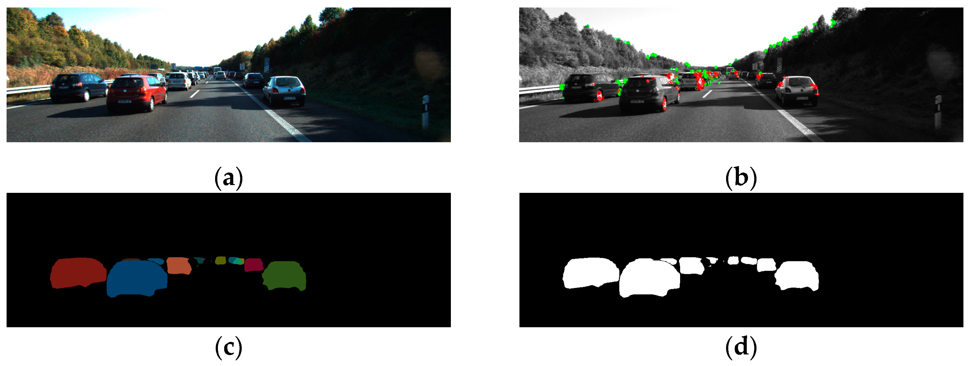
The detection results of dynamic feature points obtained are shown in Figure 2b. The red point in the figure is the dynamic feature point, while the green point is the static feature point.

3.3. Improved Instance Partitioning Network Based on YOLACT++

Mask R-CNN and its improved counterpart, MS R-CNN, are currently the most widely used algorithms for instance segmentation. These algorithms put an emphasis on high accuracy, which ultimately results in poor performance in real time [19,25]. YOLACT [23] is a single-stage real-time instance segmentation model that was proposed by Bolya et al. at ICCV2019. This model is based on fully convolutional networks and divides segmentation of instances into two parallel operations to maintain high accuracy while simultaneously enhancing the real-time performance of the network. YOLACT [23] was developed by Bolya et al. The first branch uses the full convolutional network to generate a series of prototype masks of the original image size; the second branch predicts a vector of mask coefficients for each anchor used to encode the instance representation in the prototype space by adding an output to the target detection branch; linearly combining the work of these two branches is used to construct a high-quality mask for that instance; and the third branch uses the instance representation in the prototype space to embed the representation of the instance in the prototype space. The authors then followed up with YOLACT++, which included deformable convolution and used most of the structure of the original network. They also optimized the selection of anchor points and made some improvements to the mask evaluation, which resulted in 33.5 frames per second and 34.1% average accuracy on the MS COCO 2017 dataset using a single card of Tian XP.
Instance segmentation is a location-sensitive and location-dependent task in the discipline of computer vision. In order to make the location information more accurate, most networks obtain complete semantic information by downsampling and then recover high-resolution location information by upsampling, such as U-Net, which maintains a high-resolution feature map but leads to a large amount of valid information being lost in the process of constant upsampling and downsampling. Meanwhile, the default backbone network of YOLACT consists of ResNet101 and FPN. Although ResNet has good feature representation capability, it has limitations for small target detection and also leads to a long training time due to its too-deep layers. The overly large feature maps result in more memory usage for inference and could be more efficient for running on some small devices.
We have improved on the YOLACT++ network and propose a segmentation model YOLACT-Road for road traffic scenes, whose structure is shown in Figure 3. YOLACT-Road uses HRNet and HRFPN as the backbone network for feature extraction, and HRNet [26] can maintain a high-resolution feature map during the feature extraction process. It starts with high-resolution branches as the first stage and adds high- to low-resolution branches one by one to form more branching stages, and performs repetitive multi-scale fusion by parallelizing multiple resolution branches and repeatedly exchanging information in parallel multi-resolution branching networks throughout the process to achieve robust semantic information with fewer network layers and accurate location information with fewer network layers, reducing hardware overhead while improving accuracy. The aim is to achieve reliable semantic information and accurate location information with fewer network layers, reducing hardware overheads while improving accuracy.
Our improved method optimizes some limitation problems of YOLACT. Regarding the backbone network, HRNet + HRFPN improves the feature extraction ability compared with ResNet101 + FPN while reducing the model network depth, and can generate better quality masks for obscured and distant small targets; it optimizes the non-extreme value suppression process to improve the model inference speed. The segmentation result of the target object in the image is obtained by clipping and threshold segmentation, as shown in Figure 2c.

3.4. SLAM Algorithm for Dynamic Feature Point Filtering

The method described in Section A can distinguish the motion state of scene features. Nonetheless, because only the information of two adjacent frames is used to estimate the fundamental matrix, it is simple for the feature points in the scene to be incorrectly classified, and the dynamic region in the image cannot be obtained accurately. Consequently, it is necessary to combine the semantic boundary box in Section B to obtain the image’s dynamic region. If the number of dynamic feature points extracted in a boundary frame is greater than three, the region surrounding the frame is deemed dynamic. Figure 2d depicts the results of both dynamic and static region segmentation.
The ORB-SLAM algorithm’s existing framework consists of three threads: tracing, local mapping, and loop closing. To improve the positioning accuracy and robustness of the stereo visual SLAM algorithm in dynamic scenes, this paper incorporated a dynamic region recognition thread based on the ORB-SLAM algorithm, combined with polar constraint and instance segmentation results to segment the dynamic region in the input image. In accordance with the segmentation results of the dynamic region, the tracking thread discarded the extracted dynamic feature points. In the interframe pose estimation, only the feature points in the environment’s static area are used for positioning and the feature point map, reducing the effect of moving objects on the SLAM algorithm’s localization precision.

4. Experimental Section and Analysis

Experiments were conducted using the public KITTI odometry dataset [27] to evaluate the performance of SVD-SLAM. Real image data collected from urban, rural, and highway scenes are stored on the KITTI dataset data acquisition platform. This dataset is widely used by various perception algorithms to evaluate the performance of in-vehicle environments.
The computer hardware platform used was the BRAV-7521/JZ edge computing system, a PC with an AMD Ryzen 5 3600 3.6 GHz processor, 16 GB of RAM, and an RTX1660 graphics processing unit, while the system software platform was Ubuntu 18.04. The SLAM system is written in C++, while the threads for dynamic region segmentation are written in Python.

4.1. Traffic Scene Instance Segmentation Effect Analysis

In this study, the effectiveness of the improved YOLACT network model was verified by comparing the segmentation effect of the YOLACT model using different backbone networks and the segmentation effect of different algorithms in different scenarios.
The model inference results are displayed in Table 1; we trained the model using the same training parameters. Our model’s size was reduced by 38.64% compared to YOLACT (base). Although the model of YOLACT-darknet is smaller than that of YOLACT-R50, the average accuracy of the mask is only slightly higher than that of YOLACT-R50, which is still lower than the average accuracy of 32.41% of the improved YOLACT model (YOLACT-Road), and the inference speed increased to 46.30 frames per second. Overall, YO-LACT-Road increased inference speed and mask precision.

4.2. Comparison with ORB-SLAM2

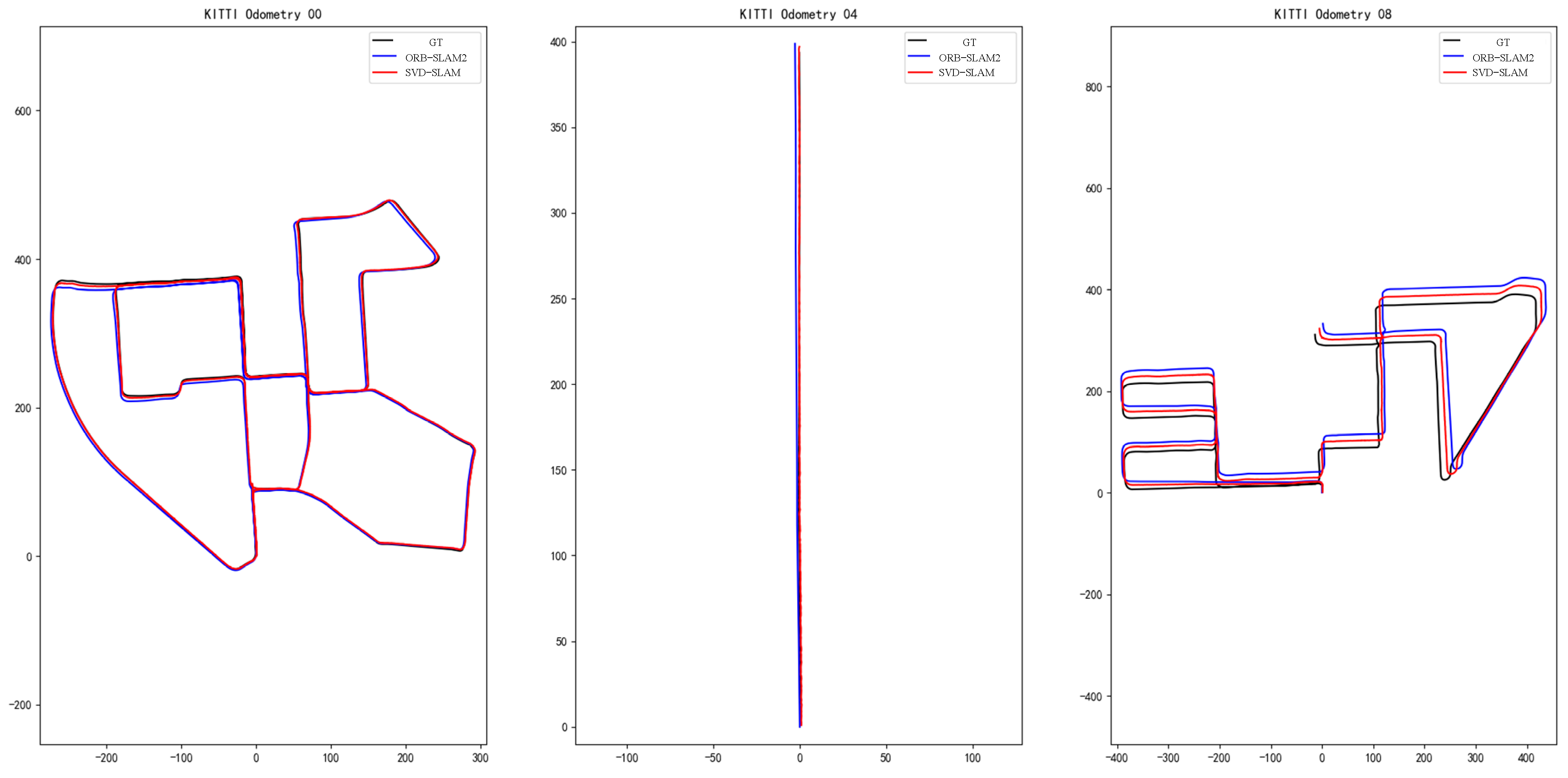
We compared the algorithm proposed in this paper to ORB-SLAM2 to determine whether it is effective because it was developed based on that algorithm’s improvement. We used the KITTI Odometry 00, 04, and 08 sequences to test the localization accuracy and robustness of the improved SLAM algorithm. The 00 sequence contains no dynamic targets, the 04 sequence contains a limited number of dynamic targets, and the 08 sequence contains a significant percentage of dynamic targets. The experimental results are displayed in Figure 4.
Absolute pose error (ATE) and relative pose error (RPE) were utilized to evaluate the positioning accuracy of the algorithm and compare it to the enhanced ORB-SLAM. ATE is the direct error between the estimated pose and the ground truth, which reflects the algorithm’s precision and the trajectory’s global consistency. The RPE includes relative translation error and relative rotation error, both of which are directly measured by odometry. The outcomes are presented in Table 2 and Table 3, where RMSE represents the root mean square error, Mean represents the mean error, and Std represents the standard deviation.
In the dataset series of low dynamic scenes, the SVD-SLAM algorithm improves the RMSE of absolute trajectory error and relative trajectory error by an average of 30.6% and 39.0%, respectively, compared to the ORB-SLAM2 algorithm, as shown in Table 2 and Table 3. In the dataset series of high dynamic scenes, the average improvement in the absolute trajectory error and relative trajectory error RMSE of this algorithm over ORB-SLAM2 is 64.5% and 62.4%, respectively, indicating that the SVD-SLAM algorithm outperforms the traditional ORB-SLAM algorithm in both low and high dynamic scenes. The trajectory is significantly more accurate in both low and high dynamic scenes.

4.3. Real-Time Analysis

Test results for the processing time of image sequences in the KITTI dataset using each module of the improved SLAM algorithm proposed in this paper are shown in Table 4. On the KITTI dataset, the tracking module takes an average of 24.7 ms, the algorithm takes an average of 66.78 ms, and the algorithm can reach a processing speed of 15 Fps. Overall, our proposed SVD-SLAM method can satisfy the real-time requirements of the system while also enhancing positioning precision and robustness.

5. Conclusions

In this paper, we present SVD-SLAM, a SLAM system for autonomous vehicles operating in a dynamic environment. It is based on dynamic feature point rejection, which can improve the localization accuracy and robustness of the stereo vision SLAM algorithm in a dynamic environment. On the basis of the open-source algorithm ORB-SLAM2, a dynamic feature point filtering thread is added to differentiate between dynamic and static image regions using instance segmentation and the feature optical flow method. Then, in the tracking thread, feature points belonging to dynamic regions are eliminated. It improves the robustness of visual SLAM in dynamic scenes by ensuring that camera localization and map construction are not affected by moving objects in the scene. Through experimental validation, the trajectory accuracy is significantly improved in both low and high dynamic scenes in the KITTI dataset, which significantly improves the localization accuracy when dynamic objects are present in the environment and guarantees localization accuracy in static scenes. Real-time system operation is compatible with the dynamic feature point filtering algorithm’s overall execution time. Consequently, the algorithm proposed in this paper can effectively improve the operation requirements of the SLAM algorithm in dynamic scenes and satisfy the localization requirements in highly dynamic scenes, such as autonomous driving.

Author Contributions

Conceptualization, L.T. and H.L.; methodology, L.T.; software, L.T. and Y.Y.; validation, L.T., Y.Y., and H.L.; formal analysis, H.L.; investigation, H.L.; resources, L.T.; data curation, L.T.; writing—original draft preparation, L.T.; writing—review and editing, Y.Y.; visualization, L.T.; supervision, Y.Y.; project administration, Y.Y.; funding acquisition, Y.Y. All authors have read and agreed to the published version of the manuscript.

Funding

This research is supported by the National Natural Science Foundation of China (51975428).

Data Availability Statement

Not applicable.

Acknowledgments

The authors are grateful to the editors and the anonymous reviewers for their insightful comments and suggestions.

Conflicts of Interest

The authors declare no conflict of interest.

References

  1. Wirbel, E.; Steux, B.; Bonnabel, S.; de La Fortelle, A. Humanoid Robot Navigation: From a Visual SLAM to a Visual Compass. In Proceedings of the 2013 10th IEEE International Conference on Networking, Sensing and Control (ICNSC), Evry, France, 10–12 April 2013; pp. 678–683. [Google Scholar]
  2. Li, Y.; Zhu, S.; Yu, Y. Improved Visual SLAM Algorithm in Factory Environment. Robot 2019, 41, 95–103. [Google Scholar]
  3. Macario Barros, A.; Michel, M.; Moline, Y.; Corre, G.; Carrel, F. A Comprehensive Survey of Visual Slam Algorithms. Robotics 2022, 11, 24. [Google Scholar] [CrossRef]
  4. Smith, R.C.; Cheeseman, P. On the Representation and Estimation of Spatial Uncertainty. Int. J. Robot. Res. 1986, 5, 56–68. [Google Scholar] [CrossRef]
  5. Fuentes-Pacheco, J.; Ruiz-Ascencio, J.; Rendón-Mancha, J.M. Visual Simultaneous Localization and Mapping: A Survey. Artif. Intell. Rev. 2015, 43, 55–81. [Google Scholar] [CrossRef]
  6. Klein, G.; Murray, D. Parallel Tracking and Mapping for Small AR Workspaces. In Proceedings of the 2007 6th IEEE and ACM International Symposium on Mixed and Augmented Reality, Nara, Japan, 13–16 November 2007; pp. 225–234. [Google Scholar]
  7. Yu, C.; Liu, Z.; Liu, X.-J.; Xie, F.; Yang, Y.; Wei, Q.; Fei, Q. DS-SLAM: A Semantic Visual SLAM towards Dynamic Environments. In Proceedings of the 2018 IEEE/RSJ International Conference on Intelligent Robots and Systems (IROS), Madrid, Spain, 1–5 October 2018; pp. 1168–1174. [Google Scholar]
  8. Mur-Artal, R.; Montiel, J.M.M.; Tardos, J.D. ORB-SLAM: A Versatile and Accurate Monocular SLAM System. IEEE Trans. Robot. 2015, 31, 1147–1163. [Google Scholar] [CrossRef]
  9. Mur-Artal, R.; Tardós, J.D. Orb-Slam2: An Open-Source Slam System for Monocular, Stereo, and Rgb-d Cameras. IEEE Trans. Robot. 2017, 33, 1255–1262. [Google Scholar] [CrossRef]
  10. Campos, C.; Elvira, R.; Rodríguez, J.J.G.; Montiel, J.M.; Tardós, J.D. Orb-Slam3: An Accurate Open-Source Library for Visual, Visual–Inertial, and Multimap Slam. IEEE Trans. Robot. 2021, 37, 1874–1890. [Google Scholar] [CrossRef]
  11. Qin, T.; Li, P.; Shen, S. Vins-Mono: A Robust and Versatile Monocular Visual-Inertial State Estimator. IEEE Trans. Robot. 2018, 34, 1004–1020. [Google Scholar] [CrossRef]
  12. Fischler, M.A.; Bolles, R.C. Random Sample Consensus: A Paradigm for Model Fitting with Applications to Image Analysis and Automated Cartography. Commun. ACM 1981, 24, 381–395. [Google Scholar] [CrossRef]
  13. Triggs, B.; McLauchlan, P.F.; Hartley, R.I.; Fitzgibbon, A.W. Bundle Adjustment—A Modern Synthesis. In Proceedings of the Vision Algorithms: Theory and Practice: International Workshop on Vision Algorithms, Corfu, Greece, 21–22 September 1999; Springer: Berlin/Heidelberg, Germany, 2000; pp. 298–372. [Google Scholar]
  14. Chapel, M.-N.; Bouwmans, T. Moving Objects Detection with a Moving Camera: A Comprehensive Review. Comput. Sci. Rev. 2020, 38, 100310. [Google Scholar] [CrossRef]
  15. Zhai, C.; Wang, M.; Yang, Y.; Shen, K. Robust Vision-Aided Inertial Navigation System for Protection against Ego-Motion Uncertainty of Unmanned Ground Vehicle. IEEE Trans. Ind. Electron. 2020, 68, 12462–12471. [Google Scholar] [CrossRef]
  16. OUYANG, Y DOF algorithm based on moving object detection programmed by Python. Mod. Electron. Tech. 2021, 44, 78–82.
  17. Wei, T.; Li, X. Binocular Vision SLAM Algorithm Based on Dynamic Region Elimination in Dynamic Environment. Robot 2020, 42, 336–345. [Google Scholar]
  18. Bescos, B.; Fácil, J.M.; Civera, J.; Neira, J. DynaSLAM: Tracking, Mapping, and Inpainting in Dynamic Scenes. IEEE Robot. Autom. Lett. 2018, 3, 4076–4083. [Google Scholar] [CrossRef]
  19. He, K.; Gkioxari, G.; Dollár, P.; Girshick, R. Mask R-Cnn. In Proceedings of the IEEE International Conference on Computer Vision (ICCV), Venice, Italy, 22–29 October 2017; pp. 2961–2969. [Google Scholar]
  20. Badrinarayanan, V.; Kendall, A.; Cipolla, R. Segnet: A Deep Convolutional Encoder-Decoder Architecture for Image Segmentation. IEEE Trans. Pattern Anal. Mach. Intell. 2017, 39, 2481–2495. [Google Scholar] [CrossRef]
  21. Liu, L.; Guo, J.; Zhang, R. YKP-SLAM: A Visual SLAM Based on Static Probability Update Strategy for Dynamic Environments. Electronics 2022, 11, 2872. [Google Scholar] [CrossRef]
  22. Liu, X.; Song, L.; Liu, S.; Zhang, Y. A Review of Deep-Learning-Based Medical Image Segmentation Methods. Sustainability 2021, 13, 1224. [Google Scholar] [CrossRef]
  23. Bolya, D.; Zhou, C.; Xiao, F.; Lee, Y.J. Yolact: Real-Time Instance Segmentation. In Proceedings of the IEEE/CVF International Conference on Computer Vision, Seoul, South Korea, 27 October–2 November 2019; pp. 9157–9166. [Google Scholar]
  24. Chen, B.; Li, S.; Zhao, H.; Liu, L. Map Merging with Suppositional Box for Multi-Robot Indoor Mapping. Electronics 2021, 10, 815. [Google Scholar] [CrossRef]
  25. Huang, Z.; Huang, L.; Gong, Y.; Huang, C.; Wang, X. Mask Scoring R-Cnn. In Proceedings of the IEEE/CVF Conference on Computer Vision and Pattern Recognition, Long Beach, CA, USA, 15–20 June 2019; pp. 6409–6418. [Google Scholar]
  26. Yu, C.; Xiao, B.; Gao, C.; Yuan, L.; Zhang, L.; Sang, N.; Wang, J. Lite-Hrnet: A Lightweight High-Resolution Network. In Proceedings of the IEEE/CVF Conference on Computer Vision and Pattern Recognition, Virtual Conference, 19–25 June 2021; pp. 10440–10450. [Google Scholar]
  27. Geiger, A.; Lenz, P.; Stiller, C.; Urtasun, R. The KITTI Vision Benchmark Suite. 2015. Available online: http://www.Cvlibs.Net/Datasets/Kitti (accessed on 24 February 2023).
Figure 1. SVD-algorithmic SLAM framework. The gray box in the image represents the original portion of ORB-SLAM2, while the green box represents the dynamic feature point filtering portion that we added.
Electronics 12 01883 g001
Figure 2. Dynamic region recognition in images. (a) Original input image. (b) Dynamic feature point detection. (c) Semantic segmentation boundary box. (d) Dynamic region segmentation results.
Electronics 12 01883 g002
Figure 3. YOLACT-Road improves instance segmentation. HRNet is the high-resolution network, HRFPN is the feature pyramid of the backbone network channel, and P3–P7 are FPN-based feature map layers. The network’s prediction head is the mask coefficient prediction head, the bounding box prediction head, the category prediction head, W, H, Ca, 4a, and Ka. The prototype network runs parallel to the prediction head. The GPU matrix operations-based binarization mask module generates masks. Mask Filters preprocesses masks.
Electronics 12 01883 g003
Figure 4. Comparison of trajectory estimation results for sequences 00, 04, 08.
Electronics 12 01883 g004
Table 1. YOLACT model performance of different backbone networks.
ModelBackboneModel Size/MBAverage Precision (AP)/%Speed/fps
YOLACT (base)ResNet101+FPN192.828.6234.71
YOLACT-R50ResNet50+FPN118.426.4547.54
YOLACT-Road(ours)HRNet+HRFPN118.332.4146.30
YOLACT-darknetDarknet53+FPN182.427.6129.32
Table 2. Comparison of absolute trajectory error (ATE).
SequencesORB-SLAM2/mSVD-SLAM/mImprovement/%
RMSEMeanStdRMSEMeanStdRMSEMeanStd
000.76620.71350.27970.53510.52450.125730.226.755.1
040.01320.00870.0570.00760.00680.002942.453.614.0
080.04420.03580.01530.01570.01280.008064.564.247.7
Table 3. Comparison of absolute trajectory error (ATE).
SequencesORB-SLAM2/mSVD-SLAM/mImprovement/%
RMSEMeanStdRMSEMeanStdRMSEMeanStd
000.01460.01170.0670.00880.01000.004039.610.454.8
040.02310.01150.02040.01320.00800.008142.730.560.1
080.4790.39100.03720.01790.01500.012162.461.767.4
Table 4. Test results of image processing time for each module.
Instance Segmentation/msORB Feature Extraction/msDynamic Point Deaction/msTracking Module/msOverall/ms
ORB-SLAM2/17.2/24.741.9
SVD-SLAM6.917.218.124.766.78
Disclaimer/Publisher’s Note: The statements, opinions and data contained in all publications are solely those of the individual author(s) and contributor(s) and not of MDPI and/or the editor(s). MDPI and/or the editor(s) disclaim responsibility for any injury to people or property resulting from any ideas, methods, instructions or products referred to in the content.