Article

A Novel Fault Diagnosis Method of Rolling Bearings Combining Convolutional Neural Network and Transformer

1
College of Engineering, South China Agricultural University, Guangzhou 510642, China
2
Key Laboratory of the Ministry of Education of China for Key Technologies for Agricultural Machine and Equipment, South China Agricultural University, Guangzhou 510642, China
*
Author to whom correspondence should be addressed.
Electronics 2023, 12(8), 1838; https://doi.org/10.3390/electronics12081838
Submission received: 22 March 2023 / Revised: 7 April 2023 / Accepted: 11 April 2023 / Published: 12 April 2023

Abstract

:
Efficient and accurate fault diagnosis plays an essential role in the safe operation of machinery. In respect of fault diagnosis, various data-driven methods based on deep learning have attracted widespread attention for research in recent years. Considering the limitations of feature representation in convolutional structures for fault diagnosis, and the demanding requirements on the quality of data for Transformer structures, an intelligent method of fault diagnosis is proposed in the present study for bearings, namely Efficient Convolutional Transformer (ECTN). Firstly, the time-frequency representation is achieved by means of short-time Fourier transform for the original signal. Secondly, the low-level local features are extracted using an efficient convolution module. Then, the global information is extracted through transformer. Finally, the results of fault diagnosis are obtained by the classifier. Moreover, experiments are conducted on two different bearing datasets to obtain the experimental results showing that the proposed method is effective in combining the advantages of CNN and transformer. In comparison with other single-structure methods of fault diagnosis, the method proposed in this study produces a better diagnostic performance in the context of limited data volume, strong noise, and variable operating conditions.

1. Introduction

With the constant progress in science and technology, the intelligence level of machinery continues to improve, which places even more demanding requirements on the intelligent fault diagnosis of machinery [1]. As one of the widely used mechanical components, rolling bearings are crucial to ensuring the safe operation of machinery [2]. Therefore, the intelligent fault diagnosis of machinery has now become the focus of research on rolling bearing faults [3].
In general, the mainstream methods of mechanical fault diagnosis are divided into model-based and data-driven methods [1,4]. Many of the prior studies were conducted by adopting the model-based approaches. Cococcioni et al. [5] assessed the state of rolling bearings through the manual selection of features and design of classifiers. Xue et al. [6] simplified the process of manual feature selection by combining Principal Component Analysis (PCA) with artificial intelligence methods. Ettefagh et al. [7] adopted K-Nearest Neighbors (k-NN) to perform distance analysis on each data sample of the bearing for determining whether it falls into a certain failure category. Song et al. [8] used wavelet packet transform to decompose the bearing vibration signal and then used support vector machine (SVM) for fault diagnosis. Similarly, there have been many classical algorithms applied to bearing fault diagnosis, such as Bayesian networks [9,10], extreme learning machines (ELM) [11], random forest [12], and empirical mode decomposition [13,14]. To construct the model and process the features, certain priori knowledge and assumptions are required by these classical methods [15].
In recent times, deep learning has emerged as a data-driven approach in numerous domains, including but not limited to computer vision [16], natural language processing [17], audio recognition [18], residual life prediction [19] and defect detection [20]. Due to its capability to automatically discern features from voluminous data, the need for human intervention is reduced [21]. Thus, a wide range of intelligent fault diagnosis techniques based on deep learning have already been proposed [22]. Among these, convolutional neural networks (CNN) have been extensively applied to assist fault diagnosis for their structural simplicity and consistent performance. Zhang et al. [23] presented a one-dimensional deep convolutional neural network with a first-layer wide convolutional kernel for the fault diagnosis of rolling bearings with time-domain signals. Wang et al. [24] proposed to extract features and visualize faults by combining symmetric dot pattern representation with CNN supporting squeeze and excitation. As for multichannel data, Guo et al. [25] proposed to carry out fault diagnosis through multilinear subspace dimensionality reduction and then extract fault features using CNN. Wang et al. [26] integrated the multimodal sensor signals collected from accelerometers and microphones for fault feature fusion and fault diagnosis through multichannel one-dimensional CNN. Recurrent neural networks (RNN) are applicable to capture temporal dependencies by processing information in sequence through a recurrent structure. Chen et al. [27] employed a variant of RNN, namely Long Short Term Memory Network (LSTM), to predict the state of mechanical devices. Zhao et al. [28] adopted sparse auto-encoder (SAE) and gated recurrent unit (GRU) for the direct fault diagnosis of bearing vibration signals. Qiao et al. [29] proposed a multiple-input fault diagnosis model based on CNN and LSTM to achieve bearing fault diagnosis under the context of variable load and variable noise with time-frequency domain signals as input.
Although CNN and RNN are both the deep learning algorithms commonly applied to fault diagnosis, they have their respective drawbacks. For example, CNN is limited in perceptual field and lacking in global information, despite its excellent performance in extracting local features [30]; RNN, which is capable to extract features for sequential information, does not support parallel computing, performs poorly in computational efficiency, is prone to gradient disappearance or explosion at the time of long sequence processing and lacks stability in training [31].
With the advancement of deep learning methodologies, a novel neural network framework, Transformer, has emerged [32]. Following the attention mechanism, it is capable to interact globally with information in each time step with other time steps, for the capture of long-range dependencies in sequential data with high parallelism and high computational power. Ding et al. [33] put forward a method of fault diagnosis for bearings based on time-frequency transformers. Weng et al. [34] integrated multiscale convolution with a one-dimensional visual Transformer to achieve satisfactory outcomes of the bearing fault diagnosis, with the raw vibration signal as input. Tang et al. [35] combined integrated learning and visual Transformer for the diagnosis of bearing fault through wavelet transform to split the vibration signal as multiple sub-signals, with each of these sub-signals as input to the transformer. He et al. [36] combined Siamese networks and transformer to improve the performance in the diagnosis of bearing fault under the context of cross-domain tasks and noisy environments.
However, there remain some problems despite the good results achieved by Transformer-based fault diagnosis in the current study. When the data is limited or poor in quality, the transformers based on attention mechanisms are more susceptible to overfitting as opposed to other deep learning models [35]. In addition, the Transformer model performs less consistently when the operating conditions change.
In the present study, which aims to enhance the accuracy and generalizability of transformer in terms of fault diagnosis, the advantages of the CNN and the Transformer are consolidated to introduce an Efficient Convolutional Transformer Network (ECTN) for bearing fault diagnosis. First of all, to improve the efficiency in extracting fault features, time-frequency representations (TFRs) are performed using the original vibration signals captured through the time-frequency processing method, namely Short Time Fourier Transform (STFT). Then, the ECTN relies on its efficient convolution module to extract the low-level features from the TFRs. Furthermore, the Transformer extracts the global features efficiently from the feature map, which enables the effective extraction of fault features and supports fault diagnosis. In the study of experimental datasets on bearings as collected from two different sources, its advantage in the accuracy and speed of inference is demonstrated through comparison with other fault diagnosis methods of different architectures. Compared to alternative sophisticated bearing fault diagnosis techniques, the proposed method attains fault diagnosis of bearings via the simple combination of Efficient convolution module and transformer module for proficiently extracting fault features from TFRs. The major contributions of this study are as follows.
(1)
A fault diagnosis model named ECTN is introduced, which employs CNN and Transformer. This model integrates the inductive bias capacity of CNN for locality with the global information interaction ability of Transformer, which is effective in extracting fault features from TFRs.
(2)
The experimental results show that the proposed approach to fault diagnosis, which is based on STFT and ECTN, can be adopted to achieve high precision with constrained training data. Meanwhile, it shows robustness to noise and capability of generalization.
The remainder of this paper is structured as follows. In Section 2 and Section 3, the proposed methodology and its constituent techniques are introduced. In Section 4 the experiments are described and the experimental results are discussed. Finally, the conclusion of this paper is drawn in Section 5.

2. Methodology

2.1. Data Processing

In terms of fault diagnosis, time-frequency analysis is widely practiced to analyze the vibration signals of machinery for fault diagnosis. In this study, the time-frequency domain analysis of vibration signals is conducted mainly through the STFT-based method. As a windowed Fourier transform, STFT can maintain a certain time resolution while achieving a higher frequency resolution, which makes it perform well in processing non-stationary vibration signals.
Capable to decompose a one-dimensional time-domain signal into a series of the time-frequency components, short-time Fourier transform is effective in describing the variation of the signal in time and frequency. It is expressed as follows,
V t , ω = + x u v u t e i ω u t d u ,
where V t , ω represents the time-frequency spectrum of the raw signal; x u indicates the raw time-domain signal; v u refers to the window function; v u t denotes the sliding window.
In this study, the Hanning window is taken as the window function of STFT, the length of the window function is set to 256, the overlap is set to 50%, and then the time domain information is segmented using a sliding window form. On this basis, the TFR output from the STFT is converted into an image and then mapped to the RGB image for matching the required input format of the neural network.

2.2. Efficient Convolutional Transformer Network

As shown in Figure 1, the Efficient Convolutional Transformer Network (ECTN) is developed in the present study to integrate convolutional neural network and Transformer. Based on the traditional convolutional neural network, an efficient convolution module is constructed to extract the local feature information in TFRs. Then, the Transformer module is used to extract global feature information. ECTN can be used to diagnose faults rapidly and accurately with less computing cost incurred. The structure of ECTN is shown in Table 1.

2.3. Efficient Convolutional Module

CNN extract features from the samples mainly through convolutional operation and analyzes the samples through multi-layered structures. Currently, the mainstream CNN models include AlexNet, GoogLeNet, VGG networks, and ResNet and some variants of ResNet-based networks [37]. These CNN-based models are usually comprised of multiple convolutional layers, pooling layers, and fully connected layers. In this study, an efficient convolutional module (EConv) is developed in ECTN.
As shown in Figure 1, ECTN involves four main stages. The downsampling layer of stage 1 consists of a layer normalization and a convolutional layer with convolutional kernel size and stride of 4. The downsampling layers in stages 2 to 4 consist of a layer normalization and a convolutional layer with convolutional kernel size and stride of 2. With the first three stages belonging to the EConv module, each stage consists of a separate downsampling layer and a stacked EConv Block. The EConv block consists mainly of a depthwise convolution layer with 7 × 7 convolutional kernels, two convolutional layers with 1 × 1 convolutional kernels, and an efficient channel attention (ECA) layer. Moreover, the residual structure is used to prevent network degradation when deep neural networks are constructed. Unlike the traditional CNNs that use batch normalization and ReLU activation functions, the EConv block uses layer normalization only after the depthwise convolution layers and the GELU activation function after the next convolutional layer.

2.3.1. Depthwise Convolution

Depthwise convolution can be performed to alleviate the computational burden compared to conventional convolution [38]. In the course of traditional convolution, every convolutional kernel executes a convolution operation with each dimension of the input feature matrix, with the number of channels in the resulting feature matrix being identical to that of convolutional kernels. Differently, each convolution kernel has one channel in depthwise convolution. Instead of combining all input channels to obtain an output feature equal to the number of input feature channels, it convolves independently for each input channel, which significantly reduces the computational workload and improves the performance of the model. In this study, the first layer of the EConv Block is a depthwise convolution with a convolution kernel size of 7 × 7.

2.3.2. Inverted Bottleneck Structure

In the classical residual network ResNet, the module is similar to a bottleneck structure in design, where the input is first down-dimensioned, then convolved, and finally up-dimensioned [39]. While the inverted bottleneck is just the opposite, where the input is first up-dimensioned, then feature extracted, and finally down-dimensioned. In the inverted bottleneck structure, the loss of high-dimensional information can be mitigated when the activation function is passed through. Gaining popularity due to MobileNet v2 proposed by Sandler et al. [40], the idea of inverted bottleneck structure has already been frequently adopted in the design of network structures. In the present study, the complex and inefficient depthwise convolution module is moved up with fewer channels, while the simple 1 × 1 convolution module is moved down to concentrate on dimensional transformation and nonlinearization operations. By changing the order, the computation workload can be effectively reduced to maintain an excellent performance.

2.3.3. Efficient Channel Attention

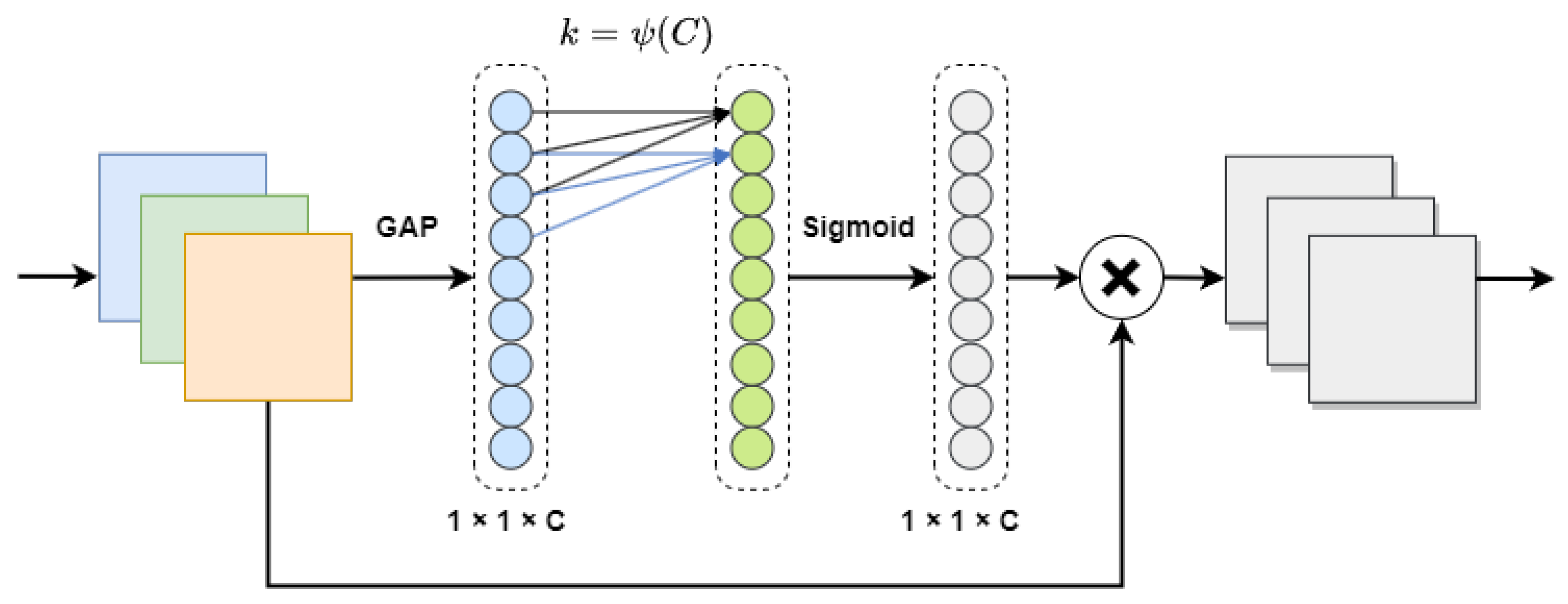
Through one-dimensional convolution, the ECA module achieves the interaction of local cross-channel information without any compromise on the dimensionality. Furthermore, it flexibly selects the size of the one-dimensional convolution kernel to determine the extent of cross-channel information interaction within the local scope [41]. By introducing a small number of parameters, ECA can achieve significant performance gains. As shown in Figure 2, ECA compresses the feature map information of a single channel into a specific value, with a feature vector [1,1,C] formed through a global average pool. Then, one-dimensional convolution is performed through a convolution kernel of size k to obtain the weight information of the corresponding channel, and feature extraction continues on these values. Finally, the information interaction between channels is completed by multiplying it with the channel feature maps corresponding to the weight information kernel.
For the parameter k, the value is proportional to the number of channels, and affectsing the coverage of cross-channel information interactions. To avoid the need for manual adjustment of the parameter k, the value of k is determined flexib adaptively fromthrough channel number C. Based on the assumingption of a mapping relationship ψ between k and C, the value of k can be determined by the following equation,
k = ψ C = log 2 C γ + b γ o d d ,
where γ = 2 , b = 1 , log 2 C γ + b γ o d d denotes the nearest log 2 C γ + b γ of odd numbers. In this study, the ECA module is computed after the 1 × 1 up-dimensioned convolution in the EConv Block.

2.4. Transformer Module

Transformer is a deep neural network model completely based on a self-attention mechanism. Different from the previous neural network models relying on a self-attention mechanism to learn and interpret relationships between sequences, it is capable to better process global information and parallelize the computation. Also, due to the architectural differences, it possesses a completely different sequential structure from the traditional CNN and RNN. Because of its excellent performance in processing long sequence information, Transformer is commonly used not only for natural language processing but also classification. However, it requires more memory and arithmetic power than the existing neural network architectures. To improve the performance of the Transformer on vision tasks, Dosovitskiy [42] proposed Vision Transformer(ViT), which has been applied to various deep learning tasks. However, ViT, as a model relying entirely on Transformer, is subject to limitations in fault diagnosis, and it does not outperform traditional neural networks in case of small sample size and complex working conditions.
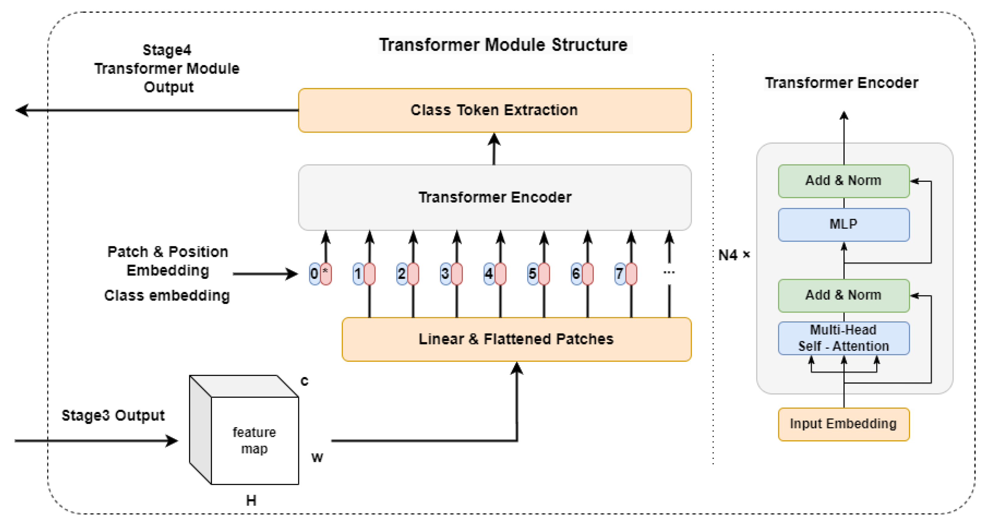
Therefore, the Transformer Module proposed in this study takes the feature maps of TFRs images outputted by EConv as input, with self-attention computation performed on the feature maps to improve the performance of the model. As shown in Figure 3, the Transformer module consists of the embedding layer, Transformer encoder, and class token extraction layer.

2.4.1. Embedding Layer

Embedding layer is intended mainly to achieve a linear projection of flattened blocks, retain the location information of the patches, and add labels to the classes. In this study, EConv outputs the feature map x R h × w × c , where h, w, and c represent the height, width, and number of channels of the feature map, respectively. The dimensions h and w of the feature map after downsampling are spread as x R h w × c , with c up-dimensioned by a convolution of size 1. Meanwhile, the class labels and location information are added before the input to the Transformer encoder, which is purposed to obtain a feature sequence containing the feature map location information and class labels as the input to the Transformer encoder. Meanwhile, to improve the stability of model training, the weights of the embedding layer are discounted from the training [43].

2.4.2. Transformer Encoder

The Transformer encoder serves as a special feature extraction structure used to extract the relevant information mainly from the sequence of the input of the embedding layer. It consists of several identical Transformer blocks, including a multi-head self-attention module with residual concatenation and layer normalization and an MLP layer. The MLP layer is comprised of a fully connected layer, a GELU activation function, and a dropout function. The hidden dimension of the fully connected layer is four times the input vector, which is then reduced to its original size by the activation function and dropout function, with the result outputted by a dropout function. The MLP layer enhances the nonlinearity of the module while improving the capability of generalization.
Among them, the multi-head self-attention is effective in learning the global features of the input vector. Since the single-head self-attention mechanism is limited to learning a single feature representation pattern, the multi-head self-attention mechanism is applied to integrate the diverse patterns learned and augment the learning capacity of the Transformer module. The self-attention formula is expressed as follows,
A t t e n t i o n Q , K , V = s o f t m a x Q · K T d k V ,
Q , K , V = X W ,
where Q, K, and V represent the query matrix, the key matrix, and the value matrix, respectively. These matrices are constructed by multiplying it by the input feature matrix X and the learnable coefficient matrix W. The dimension of Q, K, and V is denoted as d k . The multi-head self-attention mechanism learns different patterns of feature representation through multiple self-attention heads and then combines multiple output vectors. Finally, the results are outputted by linear projection. The multi-head self-attention mechanism is expressed as follows,
M u l t i H e a d Q , K , V = C o n c a t h e a d 1 , h e a d 2 , , h e a d n W ,
where W is the parameter matrix of linear projection.

2.4.3. Class Token Extraction Layer

The class token extraction layer is used to extract the class vectors from the vectors involved in Transformer encoder processing. In this study, the class vectors are taken as the input of the subsequent fault classifier, and the fault category is finalized by the output of the classifier.

3. The Proposed Fault Diagnosis Method

In order to enhance the robustness of the intelligent fault diagnosis model while improving the convergence rate and diagnostic accuracy of the proposed model, a novel technique is presented in this study for the diagnosis of faults in rolling bearings. This method is premised on ECTN, which is a hybrid model combining the advantages of both CNN and Transformer. The diagnostic process, based on ECTN, is illustrated in Figure 4.
The process of fault diagnosis is detailed as follows.
(1)
Collect the original time-domain vibration signal of the rolling bearing through the sensor.
(2)
Segment the original signal into the samples of time domain signal with fixed length and divide them proportionally into the training set, validation set, and test set.
(3)
Convert 1D time domain signal samples into TFRs by means of Short Time Fourier Transform (STFT) and then convert TFRs into 224 × 224 size images.
(4)
Train the established ECTN model and validate it on the test set through the pre-processed TFRs image training ensemble.
(5)
Output the results of fault diagnosis and determine the fault class of the sample.

4. Experiments and Result Discussion

4.1. Experimental Setup

The bearing datasets collected from Case Western Reserve University [3] and Paderborn [44] were taken as the primary datasets. Then, a sequence of experiments was determined to verify the diagnostic capability of ECTN. The hardware of our experimental platform includes an Intel® CORE™ i5-12400F CPU and NVIDIA GeForce RTX 2080 Ti GPU, with the environment of deep learning created by using CUDA 11.8, Python 3.8, and PyTorch 1.13. Initialized at 0.001, the learning rate of the model was determined using the CosineAnnealing algorithm. With the AdamW algorithm as the optimizer, iterative training was performed out for 40 epochs with a batch size of 32. Additionally, the weight decay factor was set to 0.05.

4.2. Comparison Methods and Evaluation Metrics

As shown in Table 2, the proposed fault diagnosis model was validated by selecting four different deep learning models applied to fault diagnosis as the benchmark models for comparison, including 1DCNN [23] and RNN [45] with the raw time-domain vibration signal as input, and CNN [39] and Transformer [42] with the time-domain feature map as input. Based on the same hyperparameters and data preprocessing methods used, the model structure of CNN and Transformer was adjusted to set the number of model parameters to the same level, with time-frequency feature maps as input.
The performance of a fault diagnosis model was evaluated using a confusion matrix. In case of multiple fault classes, the accuracy in the confusion matrix accurately assesses the model performance.
A c c u r a c y = T P + T N T P + F P + F N + T N ,
where TP, TN, FP, FN represent the number of true positives, true negatives, false positives and false negatives.

4.3. Case 1: CWRU Dataset

4.3.1. Description of CWRU Dataset

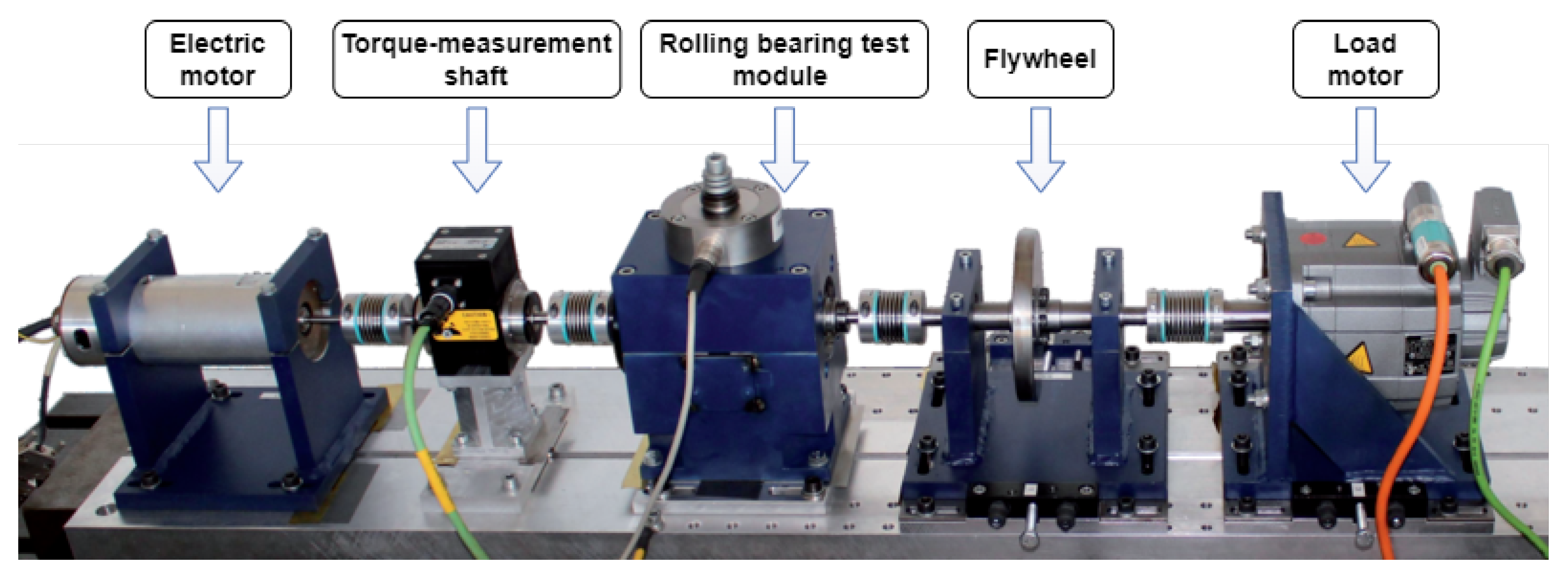
The dataset used in this section was sourced from the Case Western Reserve University (CWRU) Bearing Data Center [3]. To simulate the load, the CWRU dataset was driven directly by a 2 hp servo motor with a dynamometer mounted at the end of the drive shaft. Additionally, a torque measurement device (torque sensor with encoder) was also installed on the drive shaft, which allows the collected torque information to be fed back to the control system for adjustment of the power of the dynamometer and thus control on the load. The experimental platform is illustrated in Figure 5. The CWRU dataset collects operational data from the bearings supporting the motor rotation axis, namely bearing SKF6205 on the drive end and bearing SKF6203 on the fan end, by mounting two accelerometers at 12 o’clock in the motor housing. As shown in Figure 5, the bearing failures are EDM to simulate the rolling element, the inner ring, and outer ring failures of the bearings [46]. For each failure type, there are three failure sizes: 0.007″, 0.014″ and 0.021″. While for each failure, there are four different load cases of 0, 1, 2 and 3 hp, which correspond to the motor speed of 1797, 1772, 1750 and 1730 RPM respectively. Therefore, with the normal operation data introduced, the CWRU data set relates to 10 operating conditions in total for bearings.
As shown in Table 3, the raw experimental data were constructed using the data set of 12 kHz, which is the operation data of the drive end bearing. The data with loads 1, 2, and 3 were constructed as datasets A, B, and C. The original samples were truncated at the ratio of 0.6:0.2:0.2 and divided into the training set, validation set, and test set. Then, the one-dimensional samples of length 1024 were intercepted in each part of the original samples and obtained by the sliding window, respectively. Finally, the one-dimensional samples were converted by STFT into training, validation, and testing samples of the model. Each data set is comprised of 3000 training samples, 1000 validation samples, and 1000 test samples, with a total sample size of 5000.

4.3.2. Performance on Different Samples Sizes

The ECTN was verified by comparing a number of different fault diagnosis models at different sample sizes, with 120, 180, 300, 600, 1200, 1800, 2400, and 3000 training samples randomly selected in proportion to the training set in dataset A. Among them, the original vibration signals were used for the experiments on 1DCNN and RNN. The time-frequency feature maps were used after STFT for experiments on Transformer, CNN, and the method proposed in this paper, and the batch size was set to 2, 4, 8, 8, 16, 16, 32, 32, respectively, with equal proportions of each category in the training set for different sample sizes. Also, the corresponding validation samples were randomly selected from the validation set in dataset A by 30% of the number of training samples. In each experiment conducted at different sample sizes, the corresponding training and validation samples were used for training, and the performance of the model was tested on the test set in dataset A. Each test was repeated five times, with the results of test accuracy averaged.
As shown in Figure 6, the test accuracy of all models progressively improves and stabilizes with an increase in the size of the training sample, which evidences the high sensitivity of deep learning models to the amount of data on fault diagnosis. When the size of the training sample falls below 600, the model with time domain signal as input is low in the accuracy of test and the standard deviation is significant. Also, the training effect is inconsistent. The accuracy of the Transformer model is lower compared to other models in all cases, which is attributable to its high requirement on data volume and sample diversity, and the failure of effective fault diagnosis even with a training sample size of 3000. ECTN performs better with a limited training sample size (e.g., 120 and 180), with the accuracy reaching 95.2% and 95.6%, which are 2.64% and 0.84% higher than the CNN model, respectively. Also, the standard deviation is reduced by 0.29 and 0.6, and the training speed is 84.105 seconds faster, and the performance in stability and accuracy is better than other models. Figure 7 and Figure 8 illustrates the classification effect given 120 and 180 training samples. With a sufficient amount of data and a training sample size of 3000, the accuracy of all models exceeds 97% except for the Transformer model, and the test accuracy achieved by the proposed method reaches 100%.
Table 4 shows the results as obtained when the test is conducted on 3000 training samples, i.e., all the training samples of dataset A. It can be found out from the table that the proposed method achieves a good balance between training time and test accuracy when the order of magnitude of the number of parameters is identical and the same data processing method is used. Also, as shown in Figure 9, the proposed method tends to stabilize and converge gradually after 25 iterations of training, while the training loss of the model is consistently more significant than the validation loss. It is indicated that the structure and regularization of the model are effective in suppressing overfitting and that the model performs well in robustness and generalization.

4.3.3. Performance on Noisy Environment

This section elaborates on the performance of the model in fault diagnosis given a varying level of noise. To this end, the Gaussian white noise with different signal-to-noise ratios is introduced to the original signal. The signal-to-noise ratio is expressed as follows,
S N R d B = 10 log 10 P signal P niose ,
where P signal represents the signal strength, P niose refers to the strength of the noise, S N R d B denotes the signal-to-noise ratio, which is defined as the ratio of the raw signal to the noise signal and expressed in decibels (dB).
The introduc added signal-to-noise ratio ranges from −4 dB to 10 dB. According to Equation (7), we first convert the input signal-to-noise ratio to amplitude units, then calculate the average power P signal of the original data segment needed, and then calculate the power P niose of the Gaussian white noise signal that needs to be added to the data. Finally, Gaussian white noise obeying normal distribution is generated, and the noise is added to the data to get the data with Gaussian white noise added. We use Dataset A is taken as our base dataset and the experimental setup is the same as described in the previous section. Each experiment was repeated five times and the averaged was taken.
Figure 10 shows the experimental results obtained under different noise conditions. Due to the reduction in signal-to-noise ratio, there is a concomitant reduction in diagnostic accuracy regardless of the methods adopted. Despite a reduction in signal-to-noise ratio to −4, the method proposed in this paper maintains a higher accuracy of prediction than 90%. Evidently, the proposed method outperforms other benchmark models in the robustness to noise, especially when the signal-to-noise ratio is lower and the amplitude of noise is greater. Moreover, it is less disturbed under different noise conditions and the diagnostic results are more consistent.

4.3.4. Performance on Domain Generation

In order to evaluate the performance of the proposed model in domain generalization, cross-domain experiments were designed. Previously, the experiments were conducted using dataset A with a fixed load of 1 hp, which is inconsistent with the load variation in practice. Therefore, a dataset was chosen for training and validation before the test was conducted on a different dataset. On the previously designed dataset, there are six different cases involved, namely A–B, A–C, B–A, B–C, C–A, and C–B. The experimental configuration, as described in the preceding section, was replicated five times for each test, with the resultant values averaged for analysis. As shown in Table 5, the proposed method performs better than the other benchmark models in domain generalization under various operating conditions. The average accuracy of the Transformer model reaches only 64.72%, which is the lowest in the test. Both 1DCNN and RNN achieve an average accuracy of less than 90% and more than %. The CNN with TFRs as input and the ECTN model proposed in this paper outperform 1DCNN and RNN.
Between the data sets A, B and C, the working conditions between A and C are more different, and the speed and load changes are more significant (A: 1772[rpm] → C: 1730[rpm], A: 1[hp] → C: 3[hp]). Thus, the accuracy of the experiment is reduced in the two cases of A–C and C–A. The accuracy of ECTN achieved in these two experiments is 92.38% and 85.53%, respectively, which is 10.38% and 3.03% higher than the second-ranking CNN, respectively. As can be seen clearly from Table 5 and Figure 11, the average accuracy achieved by the ECTN proposed in this paper is 94.74%, which is higher compared to other benchmark models, demonstrating its excellent performance in domain generalization.

4.3.5. Ablation Experiments

Ablation experiments were conducted on the basis of cross-domain experiments to validate the proposal of combining efficient convolution and Transformer structures in the model. The experimental design is the same as described in the preceding section, with the EConv module and Transformer module removed from the model and then replaced with the relative structures, respectively.
As shown in Table 6, (w/o) stands for without. It can be found out that the hybrid network that integrates efficient convolution with Transformer structure significantly enhance the accuracy of the model in cross-domain fault diagnosis.

4.4. Case 2: PU Dataset

4.4.1. Description of PU Dataset

In this subsection, the proposed model is validated using the Paderborn University bearing dataset (PU) [44]. As shown in Figure 12, the PU bearing experimental rig consists of five parts. The test bearing is a 6203 deep groove ball bearing damaged due to human factors and operations. There were four different operating conditions set by changing the radial force on the test bearing, as well as the speed and load torque of the drive system. As shown in Table 7, three operating conditions in the PU data set with a rotation speed of 1500 rpm were selected to construct data sets D, E, and F. The data files used in the study are shown in Table 8 from which it can be seen that datasets D, E and F contain the vibration signals collected from healthy, human damaged, and physically damaged bearings, which are divided into six categories. Similarly, the dataset is proportionally divided into a training set, a validation set, and a test set, as shown in Table 9.

4.4.2. Results and Analysis

As shown in Table 10, the proposed method was validated by conducting cross-domain comparative experiments on datasets D, E and F with a 3000 sample sizes of 1800 training samples. The experimental setup is the same as described in the previous section, where D-D denotes the training on dataset D and then the test on D, which corresponds to the accuracy of fault diagnosis as achieved under fixed operating conditions. Under the fixed working conditions, the proposed method outperforms other methods and can identify the fault categories effectively. However, it is usually not outstanding in diagnosing these two categories of faults with labels 0 and 4. The classification effects are shown in Figure 13 and Figure 14, respectively. In cross-domain experiments, the test results of the method are better compared to other benchmark methods. On datasets D, E and F, the proposed method outperforms 1DCNN, RNN, and CNN in average accuracy by 2–3%, and it outperforms Transformer by 12.98%. The experimental results show that the proposed method also outperforms other benchmark models on complex datasets.

5. Conclusions

In this paper, an end-to-end intelligent fault diagnosis method is proposed on the basis of an Efficient Convolutional Transformer Network (ECTN). Firstly, it performs STFT processing on the vibration signal of rolling bearings to obtain TFRs images. Then, the TFRs are inputted into ECTN to extract fault features and determine the fault categories. The proposed ECTN shows the following two characteristics. On the one hand, ECTN relies on the multi-headed attention mechanism of Transform to improve the performance of the network in parallel computing and reduce the computational cost. Meanwhile, the efficient convolution module in it can be used to extract local features from TFRs accurately and improve the stability of the network. On the other hand, the fault feature information is effectively extracted from TFRs for fault diagnosis by simply combining the traditional convolution and deformer Transformer.
Its effectiveness is verified through the comparative experiments conducted on two different datasets. On dataset I, the accuracy of fault diagnosis can reach above 90% even in the case of strong noise and small sample size. On dataset II, the average accuracy of fault diagnosis exceeds 90% in cross-domain experiments. Compared with other fault diagnosis models based on a single structure, the method proposed in this study achieves higher diagnostic accuracy and better generalization performance given insufficient sample size and complex operating conditions. The experimental results show that ECTN, which combines the advantages of convolutional neural network and Transformer, performs well in diagnostic accuracy and training speed.
Nonetheless, there are still some limitations facing the method proposed in this paper. Although the various samples in the dataset used in this paper are fully balanced, it is common to have unbalanced datasets in practice. Also, the method is not suitable for processing multi-channel input signals. Therefore, the focus of our future work is to study the performance of ECTN in fault diagnosis on unbalanced datasets, with multi-channel input signals used to optimize the fault diagnosis method and enhance the performance of the model in generalization.

Author Contributions

Conceptualization, Z.Z.; methodology, W.L.; software, J.Z. and G.Z.; validation, W.L., H.H. and M.P.; formal analysis, J.Z.; investigation, W.L. and J.Z.; resources, W.L.; data curation, W.L.; writing—original draft preparation, W.L.; writing—review and editing, W.L. and Z.Z.; visualization, H.H.; supervision, Z.Z.; project administration, Z.Z.; funding acquisition, Z.Z. All authors have read and agreed to the published version of the manuscript.

Funding

This research was funded by the National Key Research and Development Program [grant numbers 2020YFB1709604].

Institutional Review Board Statement

Not applicable.

Informed Consent Statement

Not applicable.

Data Availability Statement

The data used to support this study are available at the websites https://engineering.case.edu/bearingdatacenter/download-data-file and https://mb.uni-paderborn.de/kat/forschung/datacenterbearing-datacenter, accessed on 10 March 2023.

Conflicts of Interest

The authors declare no conflict of interest.

References

  1. Gao, Z.; Cecati, C.; Ding, S.X. A Survey of Fault Diagnosis and Fault-Tolerant Techniques—Art I: Fault Diagnosis With Model-Based and Signal-Based Approaches. IEEE Trans. Ind. Electron. 2015, 62, 3757–3767. [Google Scholar] [CrossRef] [Green Version]
  2. Li, J.; Huang, R.; He, G.; Liao, Y.; Wang, Z.; Li, W. A Two-Stage Transfer Adversarial Network for Intelligent Fault Diagnosis of Rotating Machinery With Multiple New Faults. IEEEASME Trans. Mechatron. 2021, 26, 1591–1601. [Google Scholar] [CrossRef]
  3. Smith, W.A.; Randall, R.B. Rolling Element Bearing Diagnostics Using the Case Western Reserve University Data: A Benchmark Study. Mech. Syst. Signal Process. 2015, 64–65, 100–131. [Google Scholar] [CrossRef]
  4. Frank, P.M.; Ding, S.X.; Marcu, T. Model-Based Fault Diagnosis in Technical Processes. Trans. Inst. Meas. Control 2000, 22, 57–101. [Google Scholar] [CrossRef]
  5. Cococcioni, M.; Lazzerini, B.; Volpi, S.L. Robust Diagnosis of Rolling Element Bearings Based on Classification Techniques. IEEE Trans. Ind. Inform. 2013, 9, 2256–2263. [Google Scholar] [CrossRef]
  6. Xue, X.; Zhou, J. A Hybrid Fault Diagnosis Approach Based on Mixed-Domain State Features for Rotating Machinery. ISA Trans. 2017, 66, 284–295. [Google Scholar] [CrossRef] [PubMed]
  7. Ettefagh, M.M.; Ghaemi, M.; Yazdanian Asr, M. Bearing Fault Diagnosis Using Hybrid Genetic Algorithm K-Means Clustering. In Proceedings of the 2014 IEEE International Symposium on Innovations in Intelligent Systems and Applications (INISTA), Alberobello, Italy, 23–25 June 2014; pp. 84–89. [Google Scholar]
  8. Song, W.; Xiang, J. A Method Using Numerical Simulation and Support Vector Machine to Detect Faults in Bearings. In Proceedings of the 2017 International Conference on Sensing, Diagnostics, Prognostics, and Control (SDPC), Shanghai, China, 16–18 August 2017; pp. 603–607. [Google Scholar]
  9. Qu, J.; Zhang, Z.; Gong, T. A Novel Intelligent Method for Mechanical Fault Diagnosis Based on Dual-Tree Complex Wavelet Packet Transform and Multiple Classifier Fusion. Neurocomputing 2016, 171, 837–853. [Google Scholar] [CrossRef]
  10. Wu, J.; Wu, C.; Cao, S.; Or, S.W.; Deng, C.; Shao, X. Degradation Data-Driven Time-To-Failure Prognostics Approach for Rolling Element Bearings in Electrical Machines. IEEE Trans. Ind. Electron. 2019, 66, 529–539. [Google Scholar] [CrossRef]
  11. Hu, Q.; Qin, A.; Zhang, Q.; He, J.; Sun, G. Fault Diagnosis Based on Weighted Extreme Learning Machine With Wavelet Packet Decomposition and KPCA. IEEE Sens. J. 2018, 18, 8472–8483. [Google Scholar] [CrossRef]
  12. Wang, Z.; Zhang, Q.; Xiong, J.; Xiao, M.; Sun, G.; He, J. Fault Diagnosis of a Rolling Bearing Using Wavelet Packet Denoising and Random Forests. IEEE Sens. J. 2017, 17, 5581–5588. [Google Scholar] [CrossRef]
  13. Van, M.; Kang, H. Bearing-ault Diagnosis Using Non-ocal Means Algorithm and Empirical Mode Decomposition-ased Feature Extraction and Two-tage Feature Selection. IET Sci. Meas. Technol. 2015, 9, 671–680. [Google Scholar] [CrossRef]
  14. Fu, Q.; Jing, B.; He, P.; Si, S.; Wang, Y. Fault Feature Selection and Diagnosis of Rolling Bearings Based on EEMD and Optimized Elman_AdaBoost Algorithm. IEEE Sens. J. 2018, 18, 5024–5034. [Google Scholar] [CrossRef]
  15. Liu, R.; Yang, B.; Zio, E.; Chen, X. Artificial Intelligence for Fault Diagnosis of Rotating Machinery: A Review. Mech. Syst. Signal Process. 2018, 108, 33–37. [Google Scholar] [CrossRef]
  16. Ren, S.; He, K.; Girshick, R.; Sun, J. Faster R-CNN: Towards Real-Time Object Detection with Region Proposal Networks. In Proceedings of the IEEE International Conference on Computer Vision, Santiago, Chile, 13–16 December 2015. [Google Scholar]
  17. Collobert, R.; Weston, J. A Unified Architecture for Natural Language Processing: Deep Neural Networks with Multitask Learning. In Proceedings of the 25th International Conference on Machine Learning, Helsinki, Finland, 5–9 July 2008. [Google Scholar]
  18. Hinton, G.; Deng, L.; Yu, D.; Dahl, G.; Mohamed, A.; Jaitly, N.; Senior, A.; Vanhoucke, V.; Nguyen, P.; Sainath, T.; et al. Deep Neural Networks for Acoustic Modeling in Speech Recognition: The Shared Views of Four Research Groups. IEEE Signal Process. Mag. 2012, 29, 82–87. [Google Scholar] [CrossRef]
  19. Zhang, A.; Wang, H.; Li, S.; Cui, Y.; Liu, Z.; Yang, G.; Hu, J. Transfer Learning with Deep Recurrent Neural Networks for Remaining Useful Life Estimation. Appl. Sci. 2018, 8, 2416. [Google Scholar] [CrossRef] [Green Version]
  20. Li, W.; Zhang, L.; Wu, C.; Cui, Z.; Niu, C. A New Lightweight Deep Neural Network for Surface Scratch Detection. Int. J. Adv. Manuf. Technol. 2022, 123, 1999–2015. [Google Scholar] [CrossRef]
  21. Salakhutdinov, R. Deep Learning. In Proceedings of the 20th ACM SIGKDD International Conference on Knowledge Discovery and Data Mining, New York, NY, USA, 24–27 August 2014; p. 1973. [Google Scholar]
  22. Zhao, R.; Yan, R.; Chen, Z.; Mao, K.; Wang, P.; Gao, R.X. Deep Learning and Its Applications to Machine Health Monitoring. Mech. Syst. Signal Process. 2019, 115, 213–237. [Google Scholar] [CrossRef]
  23. Zhang, W.; Peng, G.; Li, C.; Chen, Y.; Zhang, Z. A New Deep Learning Model for Fault Diagnosis with Good Anti-Noise and Domain Adaptation Ability on Raw Vibration Signals. Sensors 2017, 17, 425. [Google Scholar] [CrossRef] [Green Version]
  24. Wang, H.; Xu, J.; Yan, R.; Gao, R.X. A New Intelligent Bearing Fault Diagnosis Method Using SDP Representation and SE-CNN. IEEE Trans. Instrum. Meas. 2020, 69, 2377–2389. [Google Scholar] [CrossRef]
  25. Guo, Y.; Zhou, Y.; Zhang, Z. Fault Diagnosis of Multi-Channel Data by the CNN with the Multilinear Principal Component Analysis. Measurement 2021, 171, 108513. [Google Scholar] [CrossRef]
  26. Wang, X.; Mao, D.; Li, X. Bearing Fault Diagnosis Based on Vibro-Acoustic Data Fusion and 1D-CNN Network. Measurement 2021, 173, 108518. [Google Scholar] [CrossRef]
  27. Chen, Z.; Liu, Y.; Liu, S. Mechanical State Prediction Based on LSTM Neural Netwok. In Proceedings of the 2017 36th Chinese Control Conference (CCC), Dalian, China, 26–28 July 2017; pp. 3876–3881. [Google Scholar]
  28. Zhao, K.; Jiang, H.; Li, X.; Wang, R. An Optimal Deep Sparse Autoencoder with Gated Recurrent Unit for Rolling Bearing Fault Diagnosis. Meas. Sci. Technol. 2020, 31, 015005. [Google Scholar] [CrossRef]
  29. Qiao, M.; Yan, S.; Tang, X.; Xu, C. Deep Convolutional and LSTM Recurrent Neural Networks for Rolling Bearing Fault Diagnosis Under Strong Noises and Variable Loads. IEEE Access 2020, 8, 66257–66269. [Google Scholar] [CrossRef]
  30. Wu, B.; Xu, C.; Dai, X.; Wan, A.; Zhang, P.; Yan, Z.; Tomizuka, M.; Gonzalez, J.; Keutzer, K.; Vajda, P. Visual Transformers: Token-Based Image Representation and Processing for Computer Vision. arXiv 2020, arXiv:2006.03677. [Google Scholar]
  31. Kolen, J.F.; Kremer, S.C. Gradient Flow in Recurrent Nets: The Difficulty of Learning LongTerm Dependencies. In A Field Guide to Dynamical Recurrent Networks; IEEE: Piscataway, NJ, USA, 2001; pp. 237–243. ISBN 978-0-470-54403-7. [Google Scholar]
  32. Vaswani, A.; Shazeer, N.; Parmar, N.; Uszkoreit, J.; Jones, L.; Gomez, A.N.; Kaiser, L.; Polosukhin, I. Attention Is All You Need; Google Brain & University of Toronto: Toronto, ON, Canada, 2017. [Google Scholar]
  33. Ding, Y.; Jia, M.; Miao, Q.; Cao, Y. A Novel Time-requency Transformer Based on Self-ttention Mechanism and Its Application in Fault Diagnosis of Rolling Bearings. Mech. Syst. Signal Process. 2022, 168, 108616. [Google Scholar] [CrossRef]
  34. Weng, C.; Lu, B.; Yao, J. A One-Dimensional Vision Transformer with Multiscale Convolution Fusion for Bearing Fault Diagnosis. In Proceedings of the 2021 Global Reliability and Prognostics and Health Management (PHM-Nanjing), Nanjing, China, 15–17 October 2021; p. 1. [Google Scholar]
  35. Tang, X.; Xu, Z.; Wang, Z. A Novel Fault Diagnosis Method of Rolling Bearing Based on Integrated Vision Transformer Model. Sensors 2022, 22, 3878. [Google Scholar] [CrossRef]
  36. He, Q.; Li, S.; Bai, Q.; Zhang, A.; Yang, J.; Shen, M. A Siamese Vision Transformer for Bearings Fault Diagnosis. Micromachines 2022, 13, 1656. [Google Scholar] [CrossRef]
  37. Liu, Z.; Mao, H.; Wu, C.-Y.; Feichtenhofer, C.; Darrell, T.; Xie, S. A ConvNet for the 2020s. arXiv 2022, arXiv:2202.03752. [Google Scholar]
  38. Howard, A.G.; Zhu, M.; Chen, B.; Kalenichenko, D.; Wang, W.; Weyand, T.; Andreetto, M.; Adam, H. MobileNets: Efficient Convolutional Neural Networks for Mobile Vision Applications. arXiv 2017, arXiv:1704.04861. [Google Scholar]
  39. He, K.; Zhang, X.; Ren, S.; Sun, J. Deep Residual Learning for Image Recognition. In Proceedings of the 2016 IEEE Conference on Computer Vision and Pattern Recognition (CVPR), Las Vegas, NV, USA, 27–30 June 2016; pp. 770–778. [Google Scholar]
  40. Sandler, M.; Howard, A.; Zhu, M.; Zhmoginov, A.; Chen, L.-C. MobileNetV2: Inverted Residuals and Linear Bottlenecks. arXiv 2019, arXiv:1801.04381. [Google Scholar]
  41. Wang, Q.; Wu, B.; Zhu, P.; Li, P.; Zuo, W.; Hu, Q. ECA-Net: Efficient Channel Attention for Deep Convolutional Neural Networks. IEEE Trans. Neural Netw. Learn. Syst. 2020, 32, 2133–2143. [Google Scholar]
  42. Dosovitskiy, A.; Beyer, L.; Kolesnikov, A.; Weissenborn, D.; Zhai, X.; Unterthiner, T.; Dehghani, M.; Minderer, M.; Heigold, G.; Gelly, S.; et al. An Image Is Worth 16x16 Words: Transformers for Image Recognition at Scale. arXiv 2021, arXiv:2010.11929. [Google Scholar]
  43. Chen, X.; Xie, S.; He, K. An Empirical Study of Training Self-Supervised Vision Transformers. arXiv 2021, arXiv:2104.02057. [Google Scholar]
  44. Lessmeier, C.; Kimotho, J.; Zimmer, D.; Sextro, W. Condition Monitoring of Bearing Damage in Electromechanical Drive Systems by Using Motor Current Signals of Electric Motors: A Benchmark Data Set for Data-Driven Classification. Mech. Syst. Signal Process. 2016, 66, 388–399. [Google Scholar]
  45. Zhang, X.; He, C.; Lu, Y.; Chen, B.; Zhu, L.; Zhang, L. Fault Diagnosis for Small Samples Based on Attention Mechanism. Measurement 2022, 187, 110242. [Google Scholar] [CrossRef]
  46. Li, C.; Li, S.; Zhang, A.; He, Q.; Liao, Z.; Hu, J. Meta-Learning for Few-Shot Bearing Fault Diagnosis under Complex Working Conditions. Neurocomputing 2021, 439, 197–211. [Google Scholar] [CrossRef]
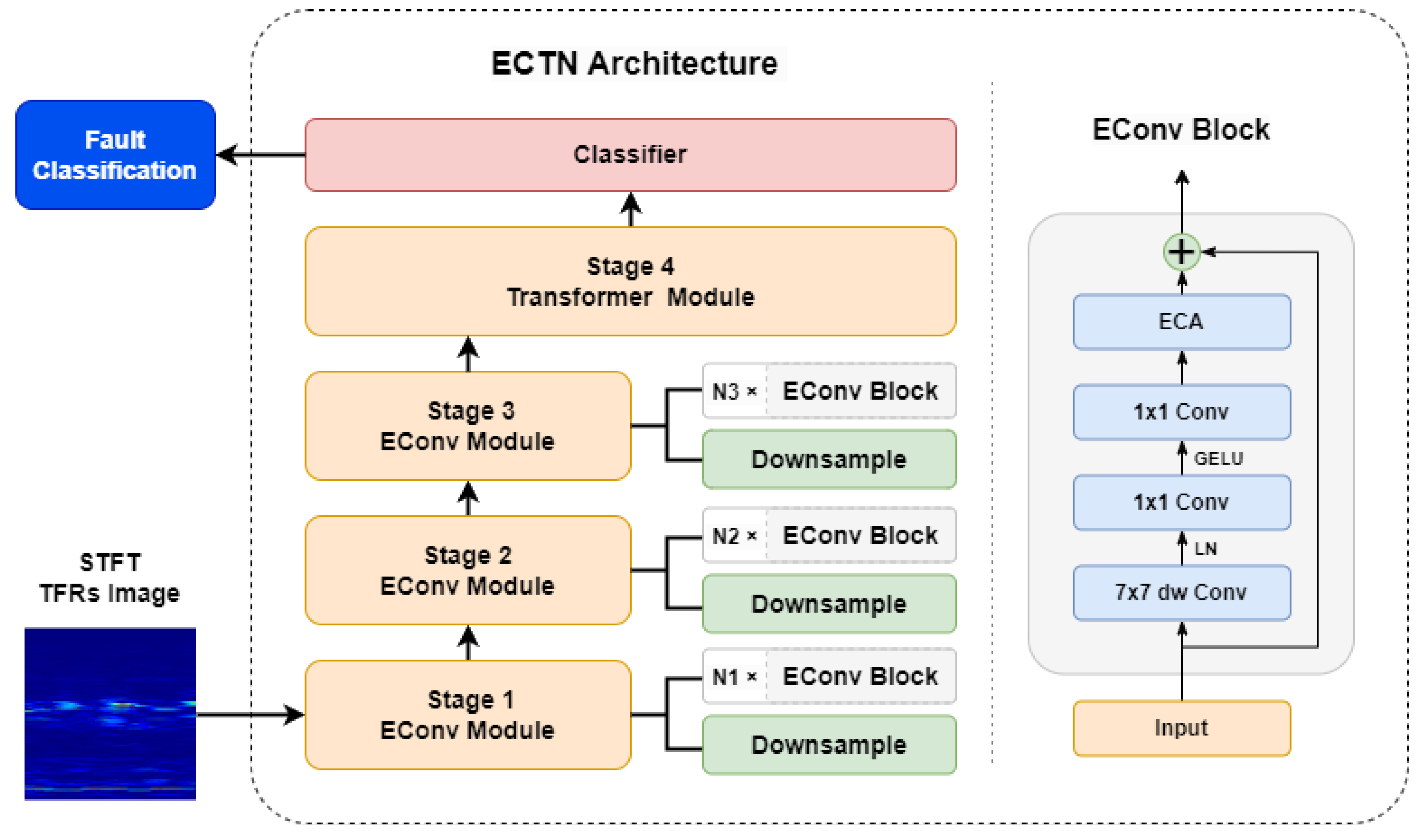
Figure 1. The proposed architecture of ECTN.
Electronics 12 01838 g001
Figure 2. The structure of the ECA module.
Electronics 12 01838 g002
Figure 3. The structure of the Transformer module.
Electronics 12 01838 g003
Figure 4. The framework of the proposed method.
Electronics 12 01838 g004
Figure 5. The bearing fault experiment platform of CWRU and the bearing fault classes.
Electronics 12 01838 g005
Figure 6. Diagnosis results of the proposed method compared with those of the comparison model for different training sample sizes.
Electronics 12 01838 g006
Figure 7. Confusion matrix results for the proposed method at (a) 180 samples and (b) 120 samples.
Electronics 12 01838 g007
Figure 8. Features visualization via t-SNE for the proposed method on (a) 180 samples and (b) 120 samples.
Electronics 12 01838 g008
Figure 9. The (a) accuracy and (b) loss of the proposed ECTN.
Electronics 12 01838 g009
Figure 10. Average diagnostic accuracy for different fault diagnosis methods under different SNRs.
Electronics 12 01838 g010
Figure 11. Accuracy histogram with 3000 training samples on CWRU.
Electronics 12 01838 g011
Figure 12. The Bearing Fault Experiment Platform of PU.
Electronics 12 01838 g012
Figure 13. Confusion matrix results for the proposed method at working conditions (a) D, (b) E, (c) F.
Electronics 12 01838 g013
Figure 14. Features visualization via t-SNE for the proposed method at working conditions (a) D, (b) E, (c) F.
Electronics 12 01838 g014
Table 1. Details of the proposed model.
StageLayer TypeOutput SizeKernel Size × Channels/Attention Heads
 Input224 × 224 × 3/
Stage1Downsample56 × 56 × 244 × 4 × 24
 N1 × EConv Block56 × 56 × 24 7 × 7 × 24 1 × 1 × 96 1 × 1 × 24 e c a × 3
Stage2Downsample28 × 28 × 482 × 2 × 48
 N2 × EConv Block28 × 28 × 48 7 × 7 × 48 1 × 1 × 192 1 × 1 × 48 e c a × 3
Stage3Downsample14 × 14 × 962 × 2 × 96
 N3 × EConv Block14 × 14 × 96 7 × 7 × 96 1 × 1 × 384 1 × 1 × 96 e c a × 9
Stage4Downsample7 × 7 × 1922 × 2 × 192
 Patch Linear & Flatten49 × 192/
 Class token & position encode50 × 192/
 N4 × Transformer Encoder50 × 19212 × 3
 Class Token Extraction1 × 192/
ClassifierFully Connected1 × Fault Class Num 
Table 2. The comparison methods.
Input TypeMethods BaseImplementation Detail
Time-based1DCNNDetails referred to [23].
 RNNDetails referred to [45].
Time-FrequencyTransformerDetails referred to [42].
 CNNDetails referred to [39].
 ECTN(our)As shown in Table 1.
Table 3. Dataset constructed based on CWRU bearing dataset.
Fault LocationNoneBallInner RingOuter RingLoadRPM
Fault Diameter(inch)00.0070.0140.0210.0070.0140.0210.0070.0140.021
Class Labels0123456789
Dataset ATrain60060060060060060060060060060011772
Valid200200200200200200200200200200
Test200200200200200200200200200200
Dataset BTrain60060060060060060060060060060021750
Valid200200200200200200200200200200
Test200200200200200200200200200200
Dataset CTrain60060060060060060060060060060031730
Valid200200200200200200200200200200
Test200200200200200200200200200200
Table 4. Performance test results with 3000 training samples on CWRU.
Input TypeModelMean AccuracyBest AccuracyStdParams NumTraining Time (s)
Time-based1DCNN97.62%98.89%0.9254,31033.867
 RNN99.54%100%0.5550,80495.649
Time-FrequencyTransformer84.82%86.2%0.872,819,146183.050
 CNN99.04%99.2%0.112,052,126366.308
 ECTN99.62%100%0.262,229,655282.203
Table 5. Mean classification accuracy(%) with 3000 training samples on CWRU.
MethodsA–BA–CB–AB–CC–AC–BAverage
1DCNN96.6285.4494.7194.6081.4684.2189.51
RNN95.8489.2594.0886.3774.0878.638637
Transformer73.3745.1073.3759.8362.10745764.72
CNN99.2082.0092.1092.3082.5096.439076
ECTN(our)99.3792.3896.9797.6085.5396.5794.74
Table 6. Ablation experiments with 3000 training samples on CWRU.
A–BA–CB–AB–CC–AC–BAverage
ECTN99.3792.3896.9797.6085.5396.5794.74
(w/o) Econv78.0062.8081.9375.1373.73843075.98
(w/o) Transformer98.9388.6797.6794.3777.0791.9391.44
(w/o) Econv & Transformer97.1077.6091.0393.0776.7090.5087.67
Table 7. Working conditions of D,E,F dataset on PU dataset.
DataSetsRotational Speed (rpm)Load Torque (Nm)Radial Force (n)Name of Setting
D15000.71000N15_M01_F10
E15000.11000N15_M07_F04
F15000.7400N15_M07_F10
Table 8. Files of the PU bearing dataset used to construct the D,E,F dataset.
Fault LocationNoneOuter RingInner Ring
File NO.K001
K002
KA01
(Artificial)
KA04
(Real)
KI01
(Artificial)
KI14
(Real)
Table 9. Dataset constructed based on PU bearing dataset.
Fault LocationNoneOuter RingInner Ring
Fault LabelsK001K002KA01KA03KI01KI14
012345
Dataset DTrain600600600600600600
Valid200200200200200200
Test200200200200200200
Dataset ETrain600600600600600600
Valid200200200200200200
Test200200200200200200
Dataset FTrain600600600600600600
Valid200200200200200200
Test200200200200200200
Table 10. Mean classification accuracy(%) with 1800 training samples on the Paderborn dataset.
MethodsD–DD–ED–FE–EE–DE–FF–FF–DF–EAverage
1DCNN90.8381.8989.8192.1380.7289.5693.0490.0090.0088.66
RNN88.9987.1789.5892.7084.7291.19903783.2285.7288.19
Transformer79.7266.5680.6780.1171.83822885.5077.3978.5678.07
CNN88.9489.0385.3993.5089.6387.67891788.5185.7888.62
ECTN(our)94.3389.9492.6197.4489.3790.2293.3991.3490.1391.05
Disclaimer/Publisher’s Note: The statements, opinions and data contained in all publications are solely those of the individual author(s) and contributor(s) and not of MDPI and/or the editor(s). MDPI and/or the editor(s) disclaim responsibility for any injury to people or property resulting from any ideas, methods, instructions or products referred to in the content.