


Advancements and Challenges in Machine Learning: A Comprehensive Review of Models, Libraries, Applications, and Algorithms


Abstract
1. Introduction
2. Types of Machine Learning
2.1. Supervised Learning
2.2. Unsupervised Learning
2.3. Semi-Supervised Learning(SSL)
2.4. Reinforcement Learning
3. Exploratory Data Analysis In Machine Learning
- Python libraries: Pandas, Numpy, Matplotlib, Seaborn, Plotly
- R libraries: ggplot2, dplyr, tidyr, caret
- Tableau
- Excel
- SAS
- IBM SPSS
- Weka
- Matlab
- Statistica
- Minitab
4. Machine Learning Problems
4.1. Classification
4.2. Regression
4.3. Clustering
4.4. Image Classification and Segmentation
4.5. Object Detection
4.6. Association Rule Learning
4.7. Ranking
- Web search results ranking
- Writing sentiment analysis
- Travel agency booking availability based on search criteria
4.8. Optimization Problems
5. Machine Learning Model Designs
5.1. Regression and Classification Problems
5.1.1. Linear Regression
5.1.2. Logistic Regression
5.1.3. Decision Tree
5.1.4. Random Forest
5.1.5. Support Vector
- 1.
- Linear Kernel
- 2.
- Polynomial Kernel
- 3.
- Radial Basis Functions Kernels
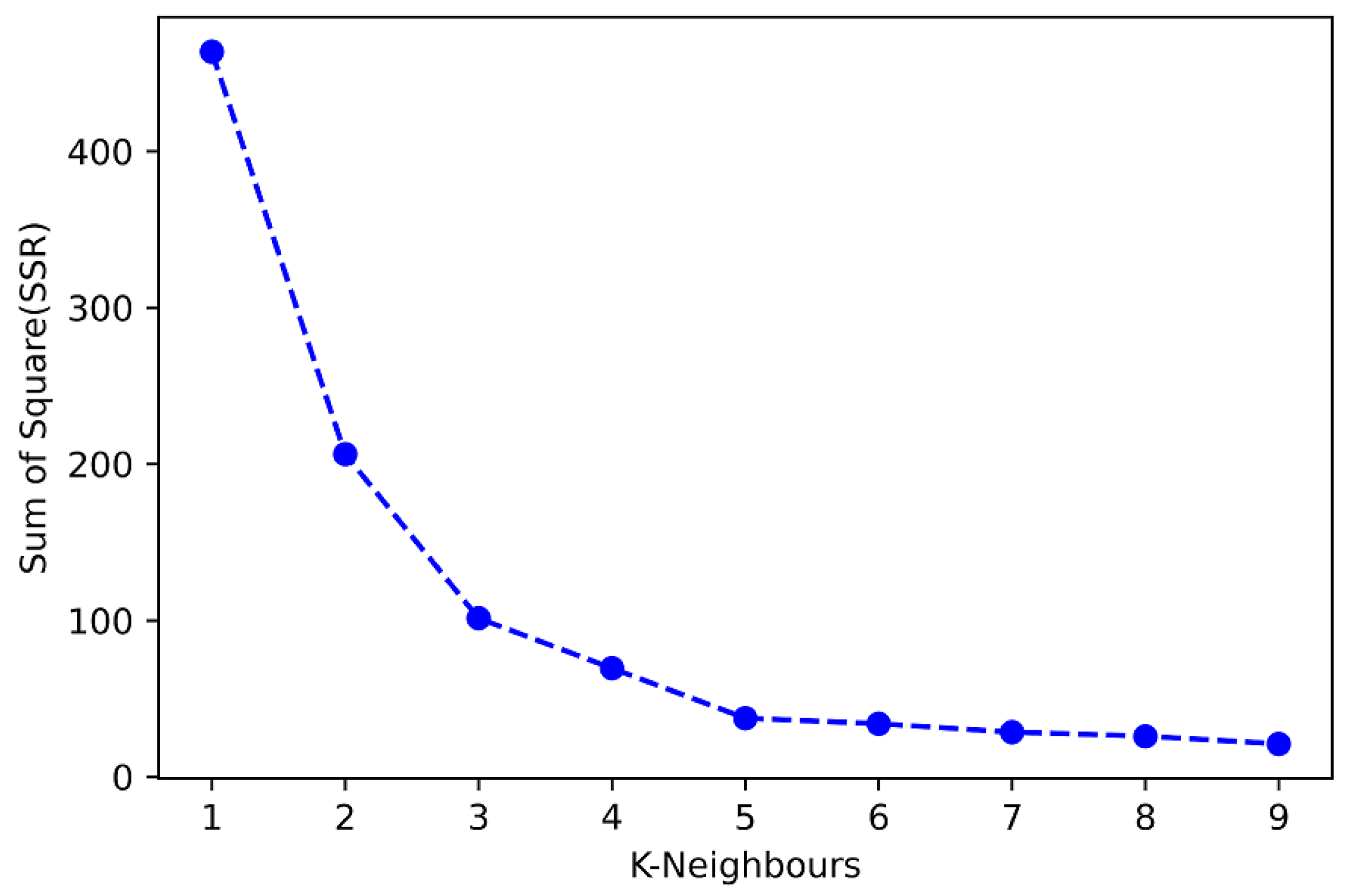
5.1.6. K-Nearest Neighbour
5.1.7. Neural Networks
- 1.
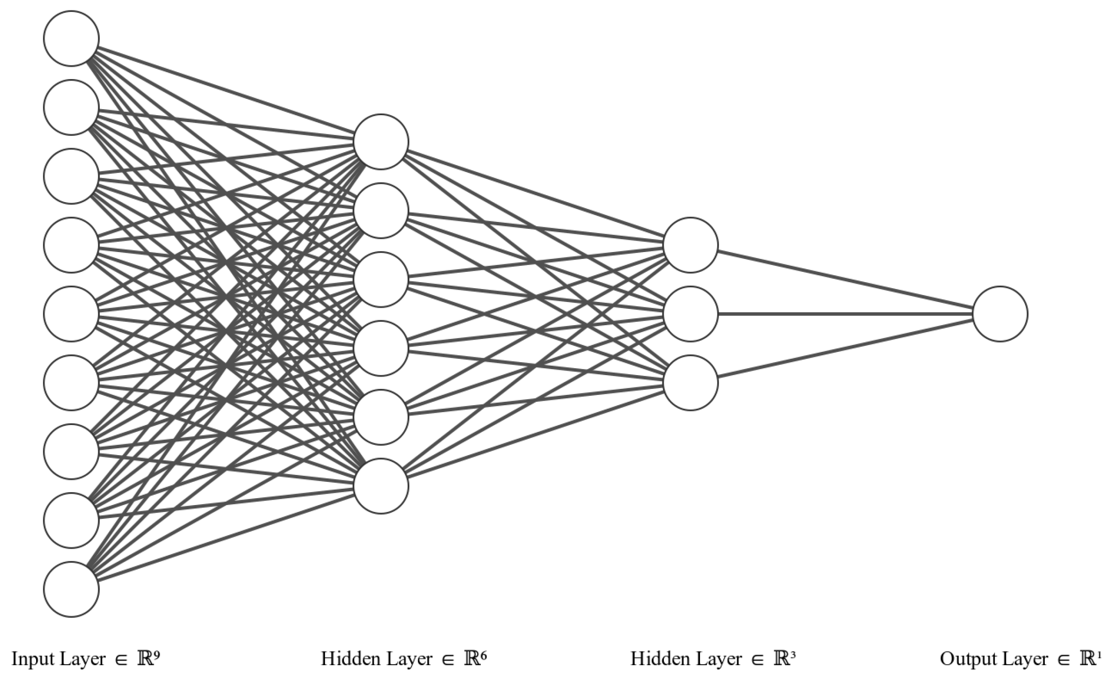
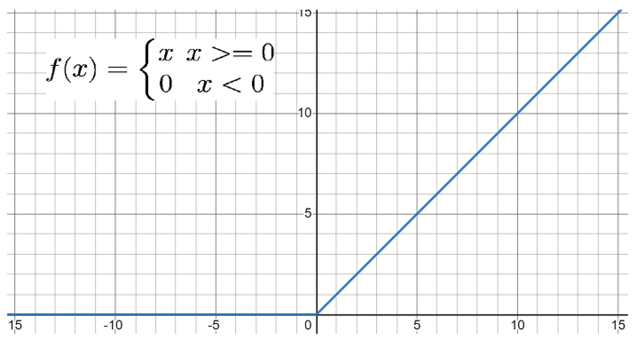
- Multi Layer Perceptron(MLP)/ Deep Neural Network: Multi layer perceptrons are similar to feed-forward neural network, but in this network there are more than one hidden layer.In the backpropogation algorithm, the output from the output layer is compared with the real value, and then weights are adjusted according to the residual. This step is repeated until there is no improvement in the output. Figure 10 shows a typical example of a deep neural network. In the real world, the data is rarely linear, so to handle non-linear data, non-linear activation functions are required. Usually two types of activation functions are applied in the MLP model: one for the hidden layer, which is generally the same for all the layers, but there is no compulsion, and one for the output layer. The most commonly used activation functions are (1) linear activation function, (2) sigmoid, and (3) relu. The output of these activation functions decides whether the neuron will fire or not. For example, in one of the most common activation functions denoted by Equation (11) the neuron is activated or fired only when the output of the neuron is greater than or equal to zero. Figure 11 shows the graphical representation of the Relu activation function. And Figure 12 representation of Sigmoid activation function.
- 2.
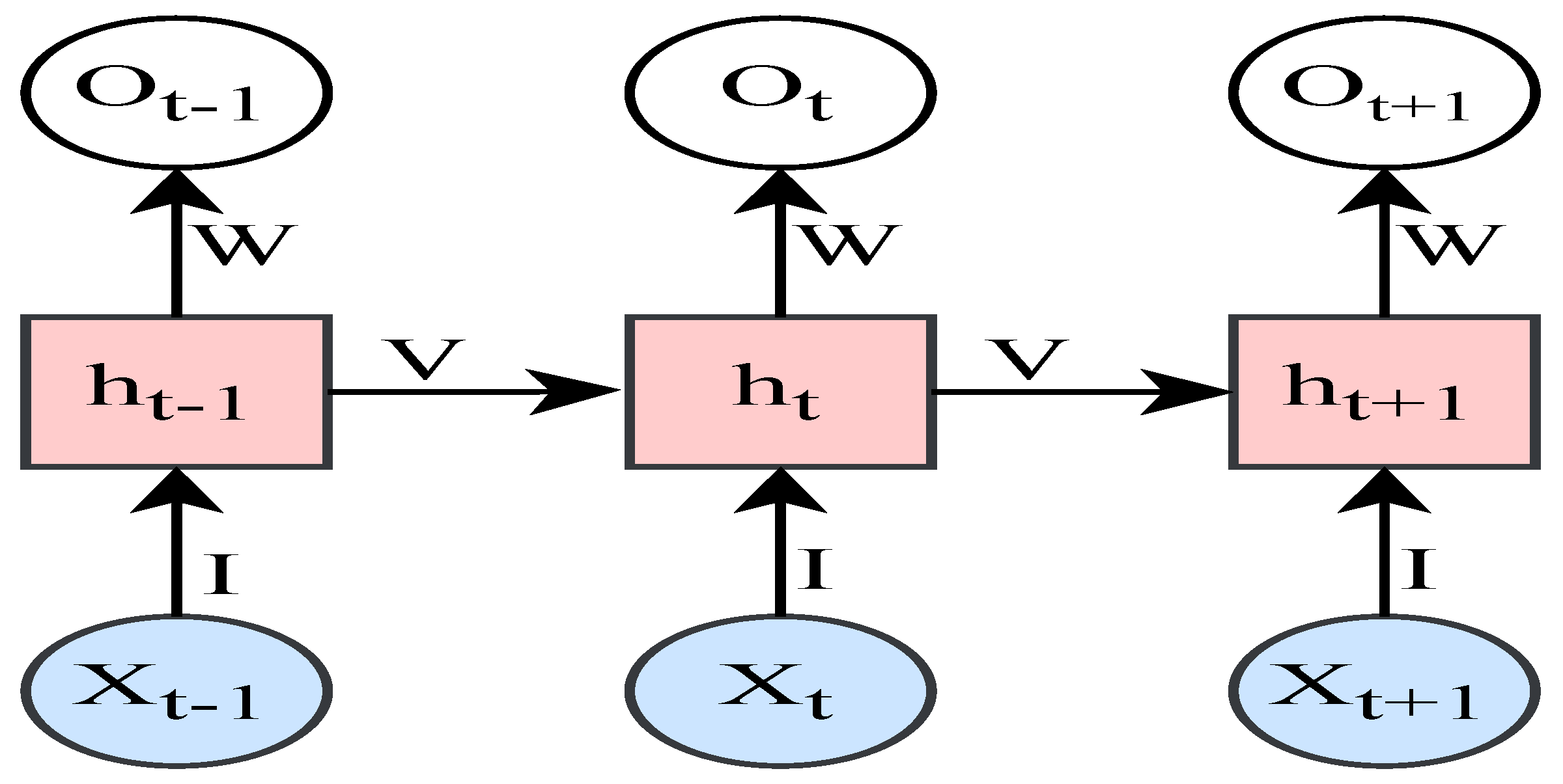
- Recurrent Neural Networks (RNN): Recurrent Neural Networks are derived from the feed-forward neural network. These networks have additional connections in their layers that enhance an ANN’s ability to learn from sequential data. This can be any form of sequential data, such as numerical time-series data or video and audio. As seen in Figure 13, a hidden layer of RNN cells passes the output to the next layer and to the adjacent cell in series. This enables the network to learn from patterns that appear in sequence. There are a few different formulations for simple RNN networks, such as the following: The W, I, and b are the weights and recurrent connection matrices.The hidden layer vector is calculated, including the recurrent connections as . The output vector is , and is the input vector.The activation functions are and [34].
- 3.
- Long Short-Term Memory (LSTM): Long short-term memory is an artificial neural network cell type that maintains memory and has input-output and forgets gates as shown in Figure 14. The LSTM is a further developed form of the RNN that incorporates the memory cell. The memory is able to carry forward over various temporal intervals and learn relations between dependent events that are not directly temporally sequential. The LSTM is also an enhanced ANN cell for overcoming the vanishing gradient problem in deep ANNs. The vanishing gradient problem refers to the exponentially smaller error signal that propagates back through the ANN during the supervised learning process as small error values (0,1) are multiplied together. Through its cell formulation, the forget gate does not have an exponential decay factor and thus counters the vanishing gradient problem. ANN using LSTM has shown record-breaking performance in language processing, such as speech recognition, in chatbots for responding to input text, and machine translation.The formulation of an LSTM cell is as follows: let W represent weight matrices and U represent the cell’s connection matrices. The components of the cell are the forget gate, input gate, output gate to the next recurrent cell in the layer, and memory cell input gate, represented respectively in the equations below.The cell state is maintained as . The output vector that goes to the next layer in the network . The variable state of the memory cell is an element of real numbers, as with the network input and . All vectors except the hidden state, output, and cell input activation vectors range from (0,1). The hidden state is in the range of [35,36,37].
- 4.
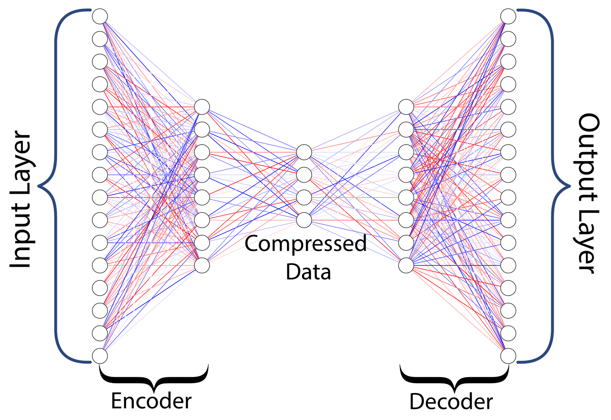
- Autoencoders: Autoencoders are an unsupervised learning technique in which neural networks are utilized for representation learning. There is a neural network architecture that imposes a bottleneck in the network and forces a compressed knowledge representation of the original input as shown in Figure 15. If the input features were independent of one another, this compression and subsequent reconstruction would be very difficult. However, if a structure exists in the data, such as correlations between input features, this structure can be learned and applied when moving the input through the network’s bottleneck. An auto-encoder comprises two parts that are encoders and decoders [38].The objective of the encoder is to compress the data in such a way that only minimal information is lost, whereas the objective of the decoder is to utilize the compressed information and regenerate the original data. Data compression, image denoising, dimensionality reduction, feature extraction, new data generation, image colorization, and anomaly detection are a few applications of autoencoders.The basic autoencoder consists of five parts: input layer, encoder hidden layer, compressed data, also known as a latent vector, decode hidden layer, and output layer. In autoencoders, the number of input features is always equal to the number of output features, and the output layer will always have fewer neurons than the input layer; otherwise, there is the possibility of data replication and there won’t be any compression. Mathematically, autoencoders can be expressed as shown in Equation (23)x is the input vector, is the encoder function, z is the compressed data, is the decoder function and is the output. Deep autoencoders are similar to basic autoencoders, but they have multiple hidden layers for encoders and decoders, where the number of hidden layers for both the encoder and the decoder should be equal and should have the same number of neurons. It’s similar to a mirror image, where the latent variable vector acts as a mirror. Some common types of autoencoders include denoising the autoencoder, the variational autoencoder, and the convolutional autoencoder [6].
- 5.
- Generative Adversarial Network (GAN): Like autoencoders, the primary application of GAN is to generate a new dataset from a given set of data. However, the architecture of GAN is very different from autoencoders. In GAN, there are two parts: the generator and discriminator. These are two different neural networks that run in parallel. The generator starts with random noise and generates a sample. Based on the feedback from the discriminator, the generator trains to generate more realistic data, and the discriminator learns from the real sample of data and the feedback from the generator. With the improvement in the performance of the generator, the performance of the discriminator deteriorates, and for a perfect generator, the accuracy of the discriminator is 50%. The basic architecture is shown in Figure 16.In GAN, two loss functions work in parallel, one for the generator and the other for the discriminator. The generator’s objective is to minimize the loss, whereas the objective of the discriminator is to maximize the loss. The mathematical formulation for the loss function is shown in Equation (24).where is the discriminators’ probability that the real data is real, is the expected value of the real data, z is the noise, is the generator output with z, is discriminator’s probability estimate that the fake data is real, is the expected output of the random samples from the generator.
- 6.
- Convolutional networks (CNN): CNNs have great applications in computer vision. These networks receive an image as input and perform a sequence of convolution and max pool operations to progressively smaller scales, descending the initial part of the ‘U’ followed by up-convolution and convolution in sequence to ascend the later part of the ‘U’. This model design has proven highly accurate at classifying objects in an image. The convolution network captures spatial and temporal dependencies in an image and performs better at classifying image data when compared to a flattened feed-forward neural network. In a convolutional network, a kernel or matrix passes over the 2-D data array and performs an up or down convolution on the data; alternatively, in a color image, the convolution kernel can be 3-dimensional. These networks are trained in supervised learning and classify images using the softmax classification technique. The ability to automatically do feature extraction and determination is the strength of these models over any competing model. The top image classification AI is based on CNNs, including LeNet, AlexNet, VGGNet, GoogleLeNet, ResNet, and ZFNet.
- 7.
- Transformer Neural Network: Transformer networks are more effective at handling long data sequences because they handle the incoming data in parallel, while standard neural networks process the data sequentially. These types of neural networks are heavily used in Natural Language (NLP) for language translation and text summarization. Transformative networks are unique in that they can prioritize different subsets of incoming data while making decisions. This is called the self-attention show in Equation (25). An attention function is a mapping between a query and a collection of key-value pairs to an output, where the query, the key-value pairs, and the result are all vectors. The output is calculated as a weighted sum of the values, where a compatibility function between the query and the corresponding key determines the weight assigned to each value.This equation computes the attention weights for a given input sequence by calculating the dot product of the query matrix Q and the key matrix K, scaling the result by the square root of the dimension of the key matrix , and applying the softmax function. The resulting attention weights are then applied to the value matrix V to weigh it and compute the output.The Transformer network consists of an encoder and a decoder. The encoder computes a sequence of hidden representations from the input sequence, utilizing several self-attention layers and feed-forward layers. After receiving the encoder’s output, the decoder generates the output sequence by attending to the encoder’s hidden representations and employing additional self-attention and feed-forward layers.Some of this network’s significant advantages are the ability to handle long sequences of data efficiently, its parallel processing capabilities, and its effectiveness in natural language processing tasks. However, it also comes with some disadvantages, including the high computational resources s required for training and the need for large amounts of data for effective training.
- 8.
- Graph Neural Network: Graph Neural Networks (GNNs) are a class of deep learning models designed to handle data structured as graphs. GNNs are particularly useful for tasks involving relational or structured data, such as social networks, citation networks, and molecular structures. The core principles of Graph Neural Networks (GNNs) and their operation in the context of graph-structured data.
- (a)
- Information diffusion mechanism: GNNs work by iteratively propagating information between nodes in the graph, simulating a process similar to information diffusion or spreading across the graph.
- (b)
- Graph processing: In a GNN, each node in the graph is associated with a processing unit that maintains a state and is connected to other units according to the graph’s connectivity.
- (c)
- State updates and information exchange: The processing units (or nodes) update their states and exchange information with their neighbors in the graph. This process is iteratively performed until the network reaches a stable equilibrium, meaning the node states no longer change significantly between iterations.
- (d)
- Output computation: Once the network reaches a stable equilibrium, the output for each node is computed locally based on its final state. This can be used for various tasks, such as node classification, link prediction, or graph classification.
- (e)
- Unique stable equilibrium: The GNN’s information diffusion mechanism is designed so that a unique stable equilibrium always exists. This ensures that the iterative process of state updates and information exchange eventually converges to a stable solution, making the GNN’s output consistent and reliable.
One simple example of a Graph Neural Network (GNN) is the Graph Convolutional Network (GCN), introduced in [39]. The GCN operates on graph-structured data and updates each node’s representation based on its neighbors’ representations. The update rule for the hidden representation of a node in a GCN can be expressed as:Here:denotes the hidden representation of nodes at the l-th layer, where is the input node features. is the adjacency matrix of the graph with added self-connections, computed as , where is the original adjacency matrix and is the identity matrix. is the degree matrix of , with . is the trainable weight matrix at the l-th layer. is an activation function, such as ReLU. In a GCN, the node representations are updated iteratively for a fixed number of layers or iterations. After the final layer, the node representations can be used for various tasks, such as node classification, link prediction, or graph classification.
5.2. Clustering
5.2.1. K-Means
5.2.2. Density Based Clustering
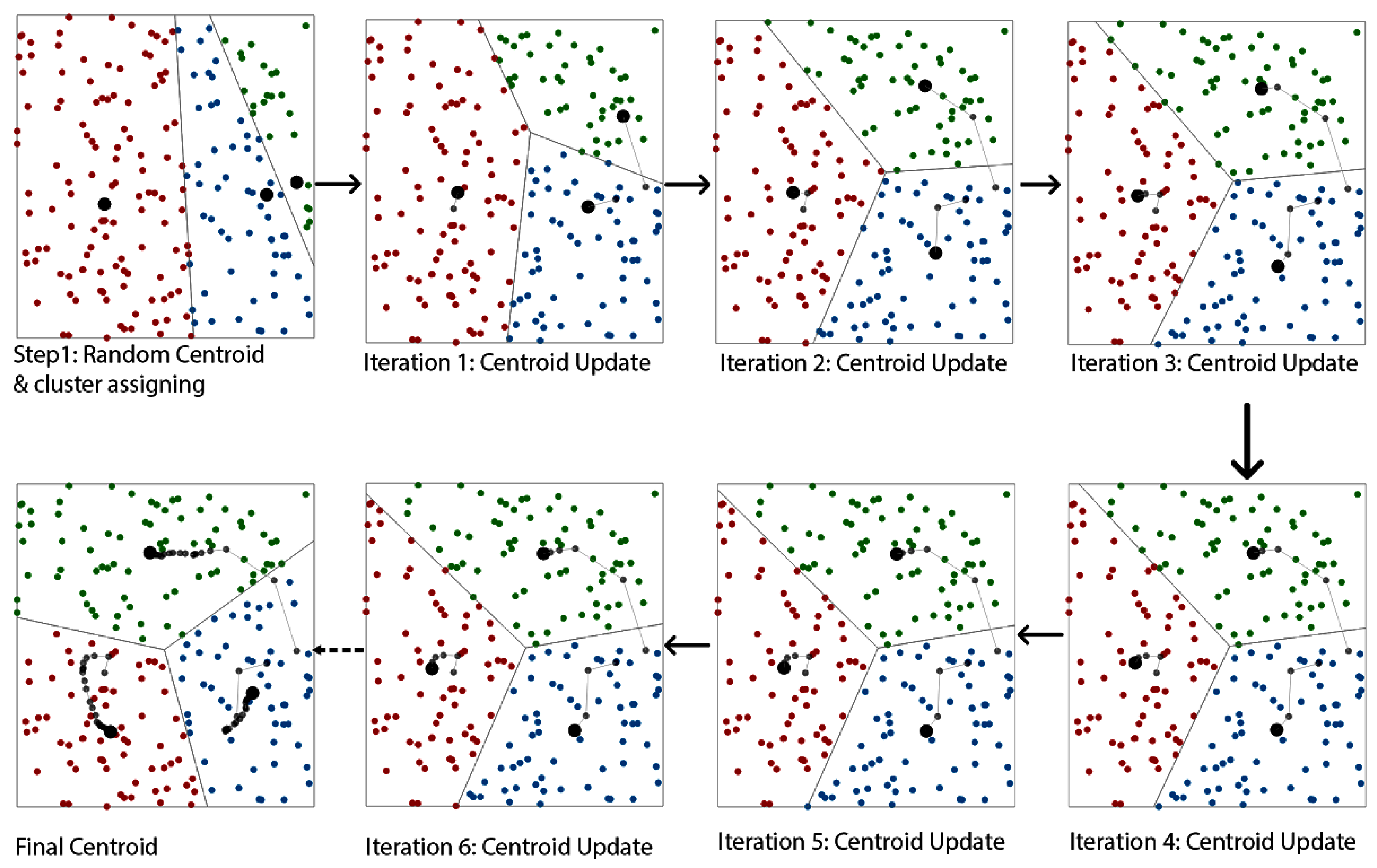
- Density-based spatial clustering of applications with noise (DBSCAN): DBSCAN starts with any object in the dataset and looks at its neighbors within a certain distance and is mostly denoted by eplison (Eps). If the points around it in that Eps are more than the minimum number of neighbors, then these points are marked as core points. The cluster is formed by core objects and non-core objects. The non-core points are part of the cluster, but they don’t extend the cluster, which means they cannot include other non-core points in the cluster. The other objects that are not part of any clusters are marked as outliers. The distance between the points is usually the Euclidean distance. The of DBSCAN is presetned in Figure 18.K-means is a centroid-based clustering algorithm, and it starts with the initialization of the number of clusters, followed by assigning a random centroid to each cluster. In the next step, we assign the points to the nearest centroid cluster, and once all the points are assigned, we update the centroid.
- Ordering Points To Identify Cluster Structure(OPTICS): OPTICS is an extended version of DBSCAN. In OPTICS two more hyperparameters are added. (1) Core Distance (2) Reachability Distance. Core distance is defined as the minimum radius value in order to mark the point as a core point, which means it will see if there is any sub-cluster within a cluster that satisfies the minimum neighbor condition. Reachability is the maxima of the core distance and the Euclidean distance between the points. Reachability and core distance are not defined for non-core points. The OPTICS algorithm works well compared to its predecessor, DBSCAN, as it is able to handle data with varying densities.
5.3. Optimization
5.3.1. Genetic Algorithm
- 1.
- Selection
- 2.
- Crossover
- 3.
- Mutation
- 4.
- Fitness function
5.3.2. Particle Swarm Optimization
5.3.3. Vortex Search
5.3.4. Simulated Annealing
5.3.5. Pattern Search
5.3.6. Artificial Bee Colony
5.4. Hyperparamter Optimization Algorithms
- 1.
- Grid Search: An exhaustive search technique that evaluates all possible combinations of hyperparameter values specified in a predefined grid [50].
- 2.
- Random Search: A simple yet effective method that samples random combinations of hyperparameter values from specified distributions, often more efficient than grid search [50].
- 3.
- Bayesian Optimization: A model-based optimization technique that uses surrogate models, typically Gaussian processes or tree-structured Parzen estimators, to guide the search for optimal hyperparameters [51].
- 4.
- Gaussian Processes: A Bayesian optimization variant that employs Gaussian processes as the surrogate model to capture the underlying function of hyperparameters and the objective [52].
- 5.
- Tree-structured Parzen Estimators (TPE): A Bayesian optimization variant that uses TPE to model the probability distribution of hyperparameters conditioned on the objective function values [53].
- 6.
- HyperBand: A bandit-based approach to hyperparameter optimization that adaptively allocates resources to different configurations and performs early stopping to improve efficiency [54].
- 7.
- Successive Halving: Successive Halving is a hyperparameter optimization approach used to identify the optimal hyperparameter combination for a particular machine learning model. The technique seeks to determine the optimal choice of hyperparameters given a constrained budget, which is often the total number of times the model can be trained and evaluated.The primary goal of successive halving is to more efficiently allocate resources by swiftly removing configurations with subpar hyperparameters. This is accomplished by running the model in parallel with various hyperparameter values and lowering the number of analyzed configurations iteratively [55].
6. Major Challenges in Machine Learning and Research Gaps
6.1. Underfitting
Underfitting Prevention Techniques
- 1.
- 2.
- Training Time: If a model has an under-fitting problem, increasing its training time can improve its accuracy [58].
- 3.
- Feature Engineering: A poor selection of features or data can mean that regardless of the model chosen, the ML will struggle to learn from the data. Feature engineering can include limiting input data through selection via principle component analysis as well as scaling input data features to the same ranges. Other feature engineering may also be done.
- 4.
- Outliers Removal: outliers can produce an unwanted effect on the training of a regression model or yield bad forecast results if taken as true input in a predictor. Filtering outliers can be necessary.
- 5.
- Increased Model Complexity: Compared with less complicated models, more sophisticated machine learning models, such as multi-layer perceptrons, can sometimes produce higher levels of accuracy. On the other hand, the training procedure itself needs to be optimized; otherwise, there is a risk of overfitting [59].
6.2. Overfitting
Overfitting Prevention Techniques
- 1.
- More training data
- 2.
- Regularisation
- 3.
- Cross Validation
- 4.
- Early Stopping
- 5.
- Dropout Layer
- 6.
- Reduce Model Complexity
- 7.
- Ensemble Learning
6.3. Model Selection
- 1.
- Akaike Information Criterion (AIC): AIC is a model selection criterion introduced by Akaike [64]. It estimates the relative quality of a set of models and is given by:where k is the number of parameters in the model, and L is the maximized value of the likelihood function for the model.
- 2.
- Bayesian Information Criterion (BIC): Also known as Schwarz Information Criterion (SIC), BIC is a model selection criterion introduced by Schwarz [65]. It is similar to AIC but has a stronger penalty for model complexity:where n is the number of samples, k is the number of parameters in the model, and L is the maximized value of the likelihood function for the model.
- 3.
- Minimum Description Length (MDL): MDL is an information-theoretic model selection criterion based on the idea of data compression [66]. It aims to find the model that can represent the data with the shortest description length (the sum of model complexity and data encoding length). MDL works well for dataset model selection. It is better than the Akaike Information Criterion (AIC) and the Bayesian Information Criterion (BIC) since it does not require assumptions about data distribution or model prior probability.
6.4. Scalability
6.5. Hyperparameter Tuning
6.6. Data availability and Missing Data
One Model Doesn’t Fit All
- 1.
- Different model architectures: Different machine learning models have different architectures and learning algorithms optimized for specific problems.
- 2.
- Model objectives: Different models have different objectives, such as minimizing mean squared error, maximizing likelihood, or maximizing accuracy. Therefore, different algorithms are used to optimize each model’s objective function.
- 3.
- Model complexity: Different models have varying levels of complexity, and a more complex model requires a different algorithm to optimize its parameters. For example, simple linear models can be optimized using gradient descent, while complex deep learning models require more sophisticated algorithms such as backpropagation.
- 4.
- Computational efficiency: Different models have different computational requirements, and some algorithms are better suited for larger datasets or distributed environments. For example, gradient boosting algorithms can handle large datasets and are suitable for distributed computing, while decision trees can become computationally expensive for larger datasets.
- 5.
- Data and problem characteristics: Different machine learning problems have varying data types, feature spaces, noise levels, underlying distributions, and objectives. Therefore, it is important to select or develop a model that is most appropriate for the specific problem at hand.
7. Generalization
Hardware Requirement
8. Machine Learning and the Programming Languages
8.1. Python
8.2. R-Programming Libraries
- Multivariate Imputation via Chained Sequences (MICE): It is handy tools for data preprocessing like handling of missing data and multivariate data imputation technique as we discussed earlier that missing data is one of the biggest challenge in machine learning models [84].
- Rpart: Its used for recursive partition for classification and regression problem. Rpart is used to build decision trees [85].
- Randomforest: This package is used to implement random forest algorithm for classification and regression task. Additionally it provide relative feature importance for the model [86].
- Caret: The caret (classification and regression training) package in R provides a wealth of resources for creating predictive models from the wide variety of existing R models. The goal of this package is to streamline the process of training and tweaking models using a wide range of modeling approaches. Methods for preparing training data, determining which variables are most important, and visualizing the resulting model are also included.SVM, random forest, bagged trees, neural networks, etc. are just some of the models that may be implemented using caret [87].
- E1071 Naive Bayes, Fourier Transform, Support Vector Machines, Bagged Clustering, etc. are just a few of the algorithms that may be put into action with the help of e1071. The most useful tool that e1071 provides is the use of support vector machines, which allow us to do classification and regression on data that would otherwise be non separable on the given dimension [88].
- Nnet: It is R library that is used to build and train neural network model for classification and regression problem [89].
8.3. Java
8.4. C++
8.5. Research Gaps
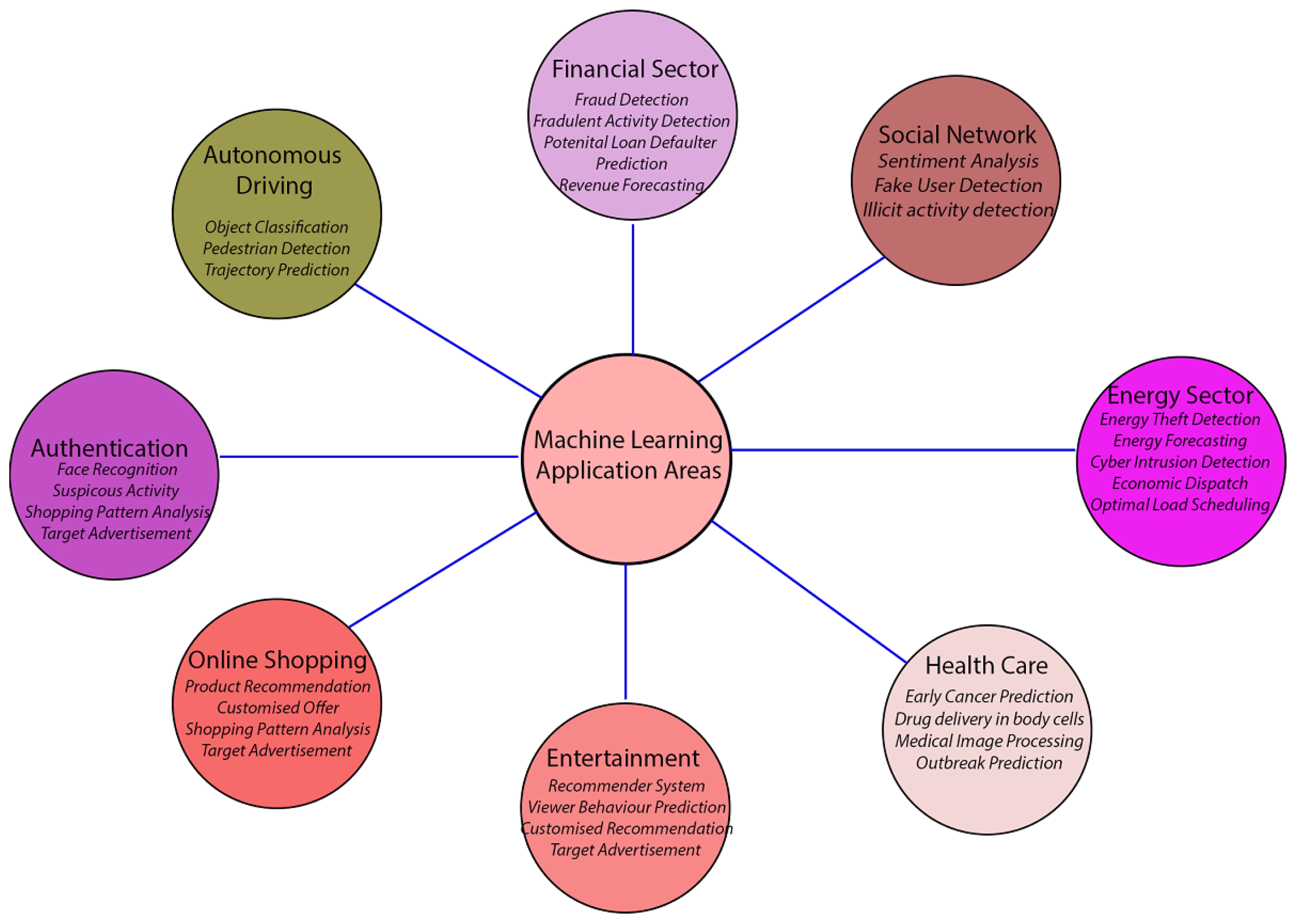
9. Applications of Machine Learning
- Energy Sector: As we discussed earlier in this article machine learning has been heavily used in the energy sector. In [126] a comparative study using random forest, support vector, naive Bayes, decision tree, and AdaBoost was performed to predict false data injection attacks in power systems. The experiment performed showed random forest yielded the most accurate results with and without feature selection and is very effective in such types of problems. However, feature selection can affect the performance of machine learning models to a great extent. A similar study was performed in [127] to detect power system faults using a decision tree, K-Nearest Neighbour and SVM. The results showed that the SVM outperformed DT and KNN algorithms with an accuracy of 91.6%. Machine learning is a very handy tool for anomaly detection in different domains, the study performed by the authors of [128] presented a study on autoencoder LSTM, Facebook prophet (time-series forecasting tool), and isolation forest predict anomaly in solar power plants. This study showed AE-LSTM can detect anomalies with high accuracy and can differentiate between anomalous signals and healthy signals.The demand for energy is increasing which is driving more households to install off-grid solar power plants. A study performed in [129] proposed a machine learning framework to maximize the consumption of solar energy using a random forest algorithm. Smart grids are vulnerable to cyberattacks. A detailed survey on various cyberattacks and their defense mechanism has been discussed in [130,131]. Machine learning may be used to identify those attacks. This includes the fake data injection attack, which can have a significant effect on AI-based smart grids [132,133]. An autoregressive integrated moving average(ARIMA) has been proposed in [134] to predict the state of charge for unknown charge and discharge rate. Also in [135] multi-layer perceptron and long short-term based model was proposed to predict battery state of charge. This work shows that the mean squared error for MLP is higher than LSTM model.
- Healthcare: Both the Naive Bayes (NB) classifier and the KNN algorithm can be used for classification problems. In this analysis [136], the authors compared the performance of KNN and Naive Bayes in predicting breast cancer. The correctness of their performance was analyzed using a cross-validation technique. According to the findings, KNN provides the highest degree of accuracy of 97.51% and had the lowest error rate compared to the NB classifier with an accuracy of 96.19%. While in [137] GAN was used to generate synthetic skin lesions. chest x-rays and renal cell carcinoma. The model was trained using 10,000 real images to generate similar synthetic images, and the performance of the models was assessed by training the model on synthetic images and another training using synthetic and real images. In [138] the study was performed on 8066 patients to predict the factors for breast cancer survivors using machine learning. In this study, random forest yielded the most accurate results and showed that the cancer stage classification, tumor size, total auxiliary lymph nodes removal, positive lymph nodes, primary treatment type, and method of diagnosis were the key factors. A comparative study to predict heart disease using logistic regression, KNN, neural network, SVM, naive Bayes, and the decision was performed in [139]. The training was performed on 297 patients sample with 13 attributes. The study showed that the SVM along with feature selection can yield up to 92.37% accuracy.
- Financial sector: It is a sector that generates a humongous amount of data every day. These data vary a lot, it can be transaction data, loan application data, borrowers’ personal data, stock data, company information data, and others. Deep learning algorithms can be used to predict stock prices [140]. The base model for the classification problem which is logistic regression can be used to predict the loan defaulter with an accuracy of 81.1% [141]. Similar research done by the authors of [142] showed that the loan default prediction accuracy can be 100% with the AdaBoost model. In the financial sector financial crisis also play a considerable role in economics. Therefore, to predict the financial crisis authors of [143] developed a hybrid model of K-means and genetic ant colony algorithm. To access the model authors used tested using the Qualitative Bankruptcy dataset [144], Polish dataset [145], and Weislaw dataset [146] data. The proposed model showed an accuracy ranging from 97.55% to 97.93% for different datasets.
- Autonomous Driving: Enhancing the safety of transportation has become feasible as a result of the quickening pace at which artificial intelligence is being incorporated into motor vehicles. It has been demonstrated that safety features such as collision detection, park assists, and lane change assist are particularly beneficial in the prevention of accidents [147,148,149]. Taking it a step further, machine learning methods for multiple object detection, trajectory prediction, motion, and speed estimation have been crucial in the development of autonomous vehicles. Even if the number of autonomous vehicles is still expanding and they are not entirely self-sufficient, additional research and data are required to demonstrate the effectiveness of such automobiles. Cybersecurity is another issue that needs to be addressed in relation to autonomous vehicles; this is due to the fact that these vehicles are equipped with a large number of sensors that provide driving assistance and that their battery management systems communicate data to the cloud. A detailed survey done in [150] presents various cyber threats and their prevention technique in autonomous vehicles.
- E-Commerce: Another industry that largely relies on machine learning is the e-commerce industry. The forecast of the product demand is done with the help of machine learning. For instance, during the winter months, sales of seasonal products like jackets are at an all-time high, and the demand for products that are used on a daily basis can skyrocket if there is any kind of severe weather alert. This kind of projection contributes to the more efficient management of supply chains [151]. In addition, online retailers often send personalized notifications to customers depending on the users’ search histories or the products they have bought in the past. The recommender system is another area in which e-commerce companies invest a lot of money. This system helps retailers propose products that are similar to ones that customers have already purchased or are considering purchasing [152,153]. In the media industry, comparable articles are suggested to users based on their reading histories. An SVM-based recommender system was proposed in ref. [154]. Some of the most prominent challenges in news recommender systems including cold start and data sparsity are discussed in ref. [155]. Furthermore, in the entertainment industry, similar shows are suggested to users depending on whether or not they have seen them or put them on their whitelists. A k-means and KNN algorithm-based recommender system is proposed in ref. [156] Both industries take a similar strategy.
- Satellite Communication: Machine learning (ML) has demonstrated significant potential in improving various aspects of satellite communication systems, making them more efficient, reliable, and adaptable. Some key ML applications in satellite communication include [157,158,159,160]:
- -
- Interference detection and mitigation: ML algorithms can identify and classify interference sources in satellite signals, enabling operators to maintain optimal system performance.
- -
- Flexible payload configuration: ML techniques, particularly deep learning, can optimize resource allocation within satellite payloads, allowing the system to adapt to changing user demands and improve capacity utilization.
- -
- Congestion prediction: ML-based forecasting can predict network congestion in satellite communication systems, enabling operators to proactively manage network resources and avoid service disruptions.
- -
- Spectrum management: ML can assist in dynamic spectrum allocation and interference mitigation, leading to more efficient use of available spectrum and better overall system performance.
- -
- Anomaly detection: ML algorithms can analyze telemetry data to detect anomalies or potential issues in satellite systems, enabling operators to address problems before they escalate.
- -
- Orbit determination and prediction: ML can improve satellite orbit prediction accuracy, facilitating better planning for satellite-based services, collision avoidance, and space debris tracking.
10. Conclusions
Author Contributions
Funding
Institutional Review Board Statement
Informed Consent Statement
Data Availability Statement
Conflicts of Interest
References
- Li, X.; Li, H.; Pan, B.; Law, R. Machine Learning in Internet Search Query Selection for Tourism Forecasting. J. Travel Res. 2021, 60, 1213–1231. [Google Scholar] [CrossRef]
- Xin, Y.; Kong, L.; Liu, Z.; Chen, Y.; Li, Y.; Zhu, H.; Gao, M.; Hou, H.; Wang, C. Machine Learning and Deep Learning Methods for Cybersecurity. IEEE Access 2018, 6, 35365–35381. [Google Scholar] [CrossRef]
- Handa, A.; Sharma, A.; Shukla, S.K. Machine learning in cybersecurity: A review. Wires Data Min. Knowl. Discov. 2019, 9, e1306. [Google Scholar] [CrossRef]
- Martínez Torres, J.; Iglesias Comesaña, C.; García-Nieto, P.J. Review: Machine learning techniques applied to cybersecurity. Int. J. Mach. Learn. Cybern. 2019, 10, 2823–2836. [Google Scholar] [CrossRef]
- James, D. Introduction to Machine Learning with Python: A Guide for Beginners in Data Science, 1st ed.; CreateSpace Independent Publishing Platform: North Charleston, SC, USA, 2018. [Google Scholar]
- Jordan, J. Introduction to Autoencoders. 2018. Available online: https://www.jeremyjordan.me/autoencoders/ (accessed on 23 January 2023).
- Chapelle, O.; Schölkopf, B.; Zien, A. Semi-Supervised Learning; The MIT Press: Cambridge, MA, USA, 2006. [Google Scholar] [CrossRef]
- Alpaydin, E. Introduction to Machine Learning, 3rd ed.; Adaptive Computation and Machine Learning; MIT Press: Cambridge, MA, USA, 2014. [Google Scholar]
- Kober, J.; Bagnell, J.A.; Peters, J. Reinforcement learning in robotics: A survey. Int. J. Robot. Res. 2013, 32, 1238–1274. [Google Scholar] [CrossRef]
- Lu, R.; Hong, S.H.; Zhang, X. A Dynamic pricing demand response algorithm for smart grid: Reinforcement learning approach. Appl. Energy 2018, 220, 220–230. [Google Scholar] [CrossRef]
- Ott, R.L.; Longnecker, M.T. Introduction to Statistical Methods and Data Analysis (with CD-ROM); Duxbury Press: Duxbury, MA, USA, 2006. [Google Scholar]
- Mathworks.com. Machine Learning with MATLAB. 2022. Available online: mathworks.com (accessed on 22 November 2022).
- Microsoft. Azure Machine Learning Documentation. 2022. Available online: https://docs.microsoft.com/en-us/azure/machine-learning/ (accessed on 6 February 2023).
- Python. Python Software Foundation. 2022. Available online: https://www.python.org/psf/ (accessed on 6 February 2023).
- r–project.org. R: What is R? 2022. Available online: https://www.r-project.org/about.html (accessed on 6 February 2023).
- Amazon. Cloud Computing Services—Amazon Web Services (AWS). 2022. Available online: https://aws.amazon.com/ (accessed on 6 February 2023).
- IBM. SPSS Software|IBM. 2022. Available online: https://www.ibm.com/analytics/spss-statistics-software (accessed on 6 February 2023).
- cs.Waikato.ac.nz. Weka 3—Data Mining with Open Source Machine Learning Software in Java. 2022. Available online: https://www.cs.waikato.ac.nz/ml/weka/ (accessed on 6 February 2023).
- DataRobot.com. DataRobot AI Cloud—The Next Generation of AI. 2022. Available online: https://www.datarobot.com/ (accessed on 5 February 2023).
- Gooogle. Cloud AutoML Custom Machine Learning Models. 2022. Available online: https://cloud.google.com/automl (accessed on 4 February 2023).
- Amazon. Machine Learning—Amazon Web Services. 2022. Available online: https://aws.amazon.com/sagemaker/ (accessed on 5 February 2023).
- KNIME.com. Open for Innovation. 2022. Available online: knime.com (accessed on 4 February 2023).
- Alteryx.com. Self-Service Analytics, Data Science & Process Automation|Alteryx. 2022. Available online: alteryx.com (accessed on 4 February 2023).
- Villegas-Mier, C.G.; Rodriguez-Resendiz, J.; Álvarez Alvarado, J.M.; Jiménez-Hernández, H.; Odry, Á. Optimized Random Forest for Solar Radiation Prediction Using Sunshine Hours. Micromachines 2022, 13, 1406. [Google Scholar] [CrossRef]
- Varma, A.; Sarma, A.; Doshi, S.; Nair, R. House Price Prediction Using Machine Learning and Neural Networks. In Proceedings of the 2018 Second International Conference on Inventive Communication and Computational Technologies (ICICCT), Coimbatore, India, 20–21 April 2018; pp. 1936–1939. [Google Scholar] [CrossRef]
- Ho, W.K.; Tang, B.S.; Wong, S.W. Predicting property prices with machine learning algorithms. J. Prop. Res. 2021, 38, 48–70. [Google Scholar] [CrossRef]
- Huynh-Cam, T.T.; Chen, L.S.; Le, H. Using Decision Trees and Random Forest Algorithms to Predict and Determine Factors Contributing to First-Year University Students’ Learning Performance. Algorithms 2021, 14, 318. [Google Scholar] [CrossRef]
- Xu, R.; Wunsch, D. Survey of clustering algorithms. IEEE Trans. Neural Netw. 2005, 16, 645–678. [Google Scholar] [CrossRef]
- Gavali, P.; Banu, J.S. Chapter 6—Deep Convolutional Neural Network for Image Classification on CUDA Platform. In Deep Learning and Parallel Computing Environment for Bioengineering Systems; Sangaiah, A.K., Ed.; Academic Press: Cambridge, MA, USA, 2019; pp. 99–122. [Google Scholar] [CrossRef]
- Géron, A. Hands-on Machine Learning with Scikit-Learn and TensorFlow: Concepts, Tools, and Techniques to Build Intelligent Systems; O’Reilly Media: Sebastopol, CA, USA, 2017. [Google Scholar]
- Edgar, T.W.; Manz, D.O. Research Methods for Cyber Security, 1st ed.; Syngress Publishing: Oxford, UK, 2017. [Google Scholar]
- Chapter 11 Random Forests|Hands-On Machine Learning with R. Available online: https://bradleyboehmke.github.io/HOML/random-forest.html (accessed on 4 February 2023).
- Burkov, A. The Hundred-Page Machine Learning Book; Andriy Burkov: Quebec, QC, Canada, 2019. [Google Scholar]
- Elman, J.L. Finding Structure in Time. Cogn. Sci. 1990, 14, 179–211. [Google Scholar] [CrossRef]
- Gers, F.A.; Schmidhuber, J.; Cummins, F. Learning to Forget: Continual Prediction with LSTM. Neural Comput. 2000, 12, 2451–2471. [Google Scholar] [CrossRef] [PubMed]
- Hochreiter, S.; Schmidhuber, J. Long Short-Term Memory. Neural Comput. 1997, 9, 1735–1780. [Google Scholar] [CrossRef] [PubMed]
- Team, G.L. Types of Neural Networks and Definition of Neural Network. 2021. Available online: https://www.mygreatlearning.com/blog/types-of-neural-networks/ (accessed on 4 February 2023).
- Fengming, Z.; Shufang, L.; Zhimin, G.; Bo, W.; Shiming, T.; Mingming, P. Anomaly detection in smart grid based on encoder-decoder framework with recurrent neural network. J. China Univ. Posts Telecommun. 2017, 24, 67–73. [Google Scholar] [CrossRef]
- He, K.; Zhang, X.; Ren, S.; Sun, J. Deep Residual Learning for Image Recognition. arXiv 2016, arXiv:1609.02907. [Google Scholar]
- Mallawaarachchi, V. Introduction to Genetic Algorithms—Including Example Code. 2020. Available online: https://www.pinterest.com/pin/introduction-to-genetic-algorithms-including-example-code–656821926880321724/ (accessed on 4 February 2023).
- Yang, X.S. Chapter 8—Particle Swarm Optimization. In Nature-Inspired Optimization Algorithms, 2nd ed.; Yang, X.S., Ed.; Academic Press: Cambridge, MA, USA, 2021; pp. 111–121. [Google Scholar] [CrossRef]
- Kennedy, J.; Eberhart, R. Particle swarm optimization. In Proceedings of the ICNN’95—International Conference on Neural Networks, Perth, Australia, 27 November–1 December 1995; Volume 4, pp. 1942–1948. [Google Scholar] [CrossRef]
- Doğan, B.; Ölmez, T. A new metaheuristic for numerical function optimization: Vortex Search algorithm. Inf. Sci. 2015, 293, 125–145. [Google Scholar] [CrossRef]
- Özkış, A.; Babalık, A. A novel metaheuristic for multi-objective optimization problems: The multi-objective vortex search algorithm. Inf. Sci. 2017, 402, 124–148. [Google Scholar] [CrossRef]
- Gharehchopogh, F.S.; Maleki, I.; Dizaji, Z.A. Chaotic vortex search algorithm: Metaheuristic algorithm for feature selection. Evol. Intell. 2022, 15, 1777–1808. [Google Scholar] [CrossRef]
- Kirkpatrick, S.; Gelatt, C.D.; Vecchi, M.P. Optimization by Simulated Annealing. Science 1983, 220, 671–680. [Google Scholar] [CrossRef]
- Černý, V. Thermodynamical approach to the traveling salesman problem: An efficient simulation algorithm. J. Optim. Theory Appl. 1985, 45, 41–51. [Google Scholar] [CrossRef]
- Torczon, V. On the Convergence of Pattern Search Algorithms. SIAM J. Optim. 1997, 7, 1–25. [Google Scholar] [CrossRef]
- Karaboga, D.; Basturk, B. A powerful and efficient algorithm for numerical function optimization: Artificial bee colony (ABC) algorithm. J. Glob. Optim. 2007, 39, 459–471. [Google Scholar] [CrossRef]
- Bergstra, J.; Bengio, Y. Random search for hyper-parameter optimization. J. Mach. Learn. Res. 2012, 13, 281–305. [Google Scholar]
- Snoek, J.; Larochelle, H.; Adams, R.P. Practical Bayesian optimization of machine learning algorithms. In Proceedings of the Advances in Neural Information Processing Systems, Lake Tahoe, NV, USA, 3–6 December 2012; pp. 2951–2959. [Google Scholar]
- Rasmussen, C.E.; Williams, C.K. Gaussian Processes for Machine Learning; MIT Press: Cambridge, MA, USA, 2006. [Google Scholar]
- Bergstra, J.; Yamins, D.; Cox, D.D. Making a science of model search: Hyperparameter optimization in hundreds of dimensions for vision architectures. In Proceedings of the 30th International Conference on Machine Learning (ICML), Atlanta, GA, USA, 16–21 June 2013; pp. 115–123. [Google Scholar]
- Li, L.; Jamieson, K.; DeSalvo, G.; Rostamizadeh, A.; Talwalkar, A. Hyperband: A novel bandit-based approach to hyperparameter optimization. arXiv 2016, arXiv:1603.06560. [Google Scholar]
- Jamieson, K.; Talwalkar, A. Non-stochastic best arm identification and hyperparameter optimization. arXiv 2015, arXiv:1502.07943. [Google Scholar]
- Tufail, S.; Batool, S.; Sarwat, A.I. A Comparative Study Of Binary Class Logistic Regression and Shallow Neural Network For DDoS Attack Prediction. In Proceedings of the SoutheastCon 2022, Mobile, AL, USA, 26 March–3 April 2022; pp. 310–315. [Google Scholar] [CrossRef]
- Zhu, X.; Vondrick, C.; Fowlkes, C.C.; Ramanan, D. Do We Need More Training Data? Int. J. Comput. Vis. 2016, 119, 76–92. [Google Scholar] [CrossRef]
- Kim, Y.J.; Choi, S.; Briceno, S.; Mavris, D. A deep learning approach to flight delay prediction. In Proceedings of the 2016 IEEE/AIAA 35th Digital Avionics Systems Conference (DASC), Sacramento, CA, USA, 25–29 September 2016; pp. 1–6. [Google Scholar] [CrossRef]
- Bustillo, A.; Reis, R.; Machado, A.R.; Pimenov, D.Y. Improving the accuracy of machine-learning models with data from machine test repetitions. J. Intell. Manuf. 2022, 33, 203–221. [Google Scholar] [CrossRef]
- Tibshirani, R. Regression Shrinkage and Selection via the Lasso. J. R. Stat. Soc. Ser. Methodol. 1996, 58, 267–288. [Google Scholar] [CrossRef]
- Prechelt, L. Early Stopping—But When? In Neural Networks: Tricks of the Trade; Orr, G.B., Müller, K.R., Eds.; Springer: Berlin/Heidelberg, Germany, 1998; pp. 55–69. [Google Scholar] [CrossRef]
- Srivastava, N.; Hinton, G.; Krizhevsky, A.; Sutskever, I.; Salakhutdinov, R. Dropout: A Simple Way to Prevent Neural Networks from Overfitting. J. Mach. Learn. Res. 2014, 15, 1929–1958. [Google Scholar]
- Guyon, I.; Elisseeff, A. An Introduction to Variable and Feature Selection. J. Mach. Learn. Res. 2003, 3, 1157–1182. [Google Scholar]
- Akaike, H. A new look at the statistical model identification. IEEE Trans. Autom. Control. 1974, 19, 716–723. [Google Scholar] [CrossRef]
- Schwarz, G. Estimating the Dimension of a Model. Ann. Stat. 1978, 6, 461–464. [Google Scholar] [CrossRef]
- Rissanen, J. Modeling by shortest data description. Automatica 1978, 14, 465–471. [Google Scholar] [CrossRef]
- Bottou, L. Large-Scale Machine Learning with Stochastic Gradient Descent. In Proceedings of the Proceedings of COMPSTAT’2010: 19th International Conference on Computational Statistics, Paris, France, 22–27 August 2010; Lechevallier, Y., Saporta, G., Eds.; Physica-Verlag HD: Heidelberg, Germany, 2010; pp. 177–186. [Google Scholar]
- Jiang, P.; Ergu, D.; Liu, F.; Cai, Y.; Ma, B. A Review of Yolo Algorithm Developments. Procedia Comput. Sci. 2022, 199, 1066–1073. [Google Scholar] [CrossRef]
- Faisal, A.; Kamruzzaman, M.; Yigitcanlar, T.; Currie, G. Understanding autonomous vehicles: A systematic literature review on capability, impact, planning and policy. J. Transp. Land Use 2019, 12, 45–72. [Google Scholar] [CrossRef]
- Fei-Fei, L.; Fergus, R.; Perona, P. One-shot learning of object categories. IEEE Trans. Pattern Anal. Mach. Intell. 2006, 28, 594–611. [Google Scholar] [CrossRef]
- Riggs, H.; Tufail, S.; Parvez, I.; Sarwat, A. Survey of Solid State Drives, Characteristics, Technology, and Applications. 2020. Available online: https://www.researchgate.net/publication/339884124_Survey_of_Solid_State_Drives_Characteristics_Technology_and_Applications (accessed on 5 February 2023).
- Tufail, S.; Qadeer, M.A. Cloud Computing in Bioinformatics: Solution to Big Data Challenge. Int. J. Comput. Sci. Eng. 2017, 5, 232–236. [Google Scholar] [CrossRef]
- Bekkerman, R.; Bilenko, M.; Langford, J. Scaling up Machine Learning: Parallel and Distributed Approaches; Cambridge University Press: Cambridge, UK, 2011. [Google Scholar]
- Parallel Processing—An Overview. Available online: https://www.sciencedirect.com/topics/computer-science/parallel-processing (accessed on 5 February 2023).
- Chollet, F. Deep Learning with Python; Manning: Shelter Island, NY, USA, 2018; ISBN 9781617294433. [Google Scholar]
- Abadi, M.; Agarwal, A.; Barham, P.; Brevdo, E.; Chen, Z.; Citro, C.; Corrado, G.S.; Davis, A.; Dean, J.; Devin, M.; et al. TensorFlow: Large-Scale Machine Learning on Heterogeneous Systems. 2015. Available online: tensorflow.org (accessed on 6 February 2023).
- Paszke, A.; Gross, S.; Massa, F.; Lerer, A.; Bradbury, J.; Chanan, G.; Killeen, T.; Lin, Z.; Gimelshein, N.; Antiga, L.; et al. PyTorch: An Imperative Style, High-Performance Deep Learning Library. In Advances in Neural Information Processing Systems 32; Wallach, H., Larochelle, H., Beygelzimer, A., d’Alché-Buc, F., Fox, E., Garnett, R., Eds.; Curran Associates, Inc.: Red Hook, NY, USA, 2019; pp. 8024–8035. [Google Scholar]
- Harris, C.R.; Millman, K.J.; van der Walt, S.J.; Gommers, R.; Virtanen, P.; Cournapeau, D.; Wieser, E.; Taylor, J.; Berg, S.; Smith, N.J.; et al. Array programming with NumPy. Nature 2020, 585, 357–362. [Google Scholar] [CrossRef]
- Hunter, J.D. Matplotlib: A 2D graphics environment. Comput. Sci. Eng. 2007, 9, 90–95. [Google Scholar] [CrossRef]
- pandas-dev/pandas: Pandas. Zenodo 2020, 21, 1–9. [CrossRef]
- Pedregosa, F.; Varoquaux, G.; Gramfort, A.; Michel, V.; Thirion, B.; Grisel, O.; Blondel, M.; Prettenhofer, P.; Weiss, R.; Dubourg, V.; et al. Scikit-learn: Machine Learning in Python. J. Mach. Learn. Res. 2011, 12, 2825–2830. [Google Scholar]
- Bradski, G. The OpenCV Library. Dr. Dobb’S J. Softw. Tools Prof. Program. 2000, 25, 120–123. [Google Scholar]
- Tufail, S.; Qadeer, M.A. Analysing data using R: An application in healthcare sector. Int. J. Comput. Sci. Eng. 2017, 5, 249–253. [Google Scholar] [CrossRef]
- Wilson, S. MICE Algorithm. 2021. Available online: https://cran.r-project.org/web/packages/miceRanger/vignettes/miceAlgorithm.html (accessed on 14 January 2023).
- Therneau, T.; Atkinson, B.; Ripley, B. Recursive Partitioning and Regression Trees [R Package Rpart Version 4.1.16]. 2022. Available online: https://rdrr.io/cran/rpart/man/ (accessed on 14 January 2023).
- Breiman, L. Random Forests. Mach. Learn. 2001, 45, 5–32. [Google Scholar] [CrossRef]
- Kuhn, M. Building Predictive Models in R Using the caret Package. J. Stat. Softw. 2008, 28, 1–26. [Google Scholar] [CrossRef]
- Meyer, D.; Dimitriadou, E.; Hornik, K.; Weingessel, A.; Leisch, F.; Chang, C.C.; Lin, C.C.; Meyer, M.D. Package ‘e1071’. R J. 2019. [Google Scholar]
- Ripley, B.; Venables, W.; Ripley, M.B. Package ‘nnet’. Package Version 2016, 7, 700. [Google Scholar]
- Health Insurance Portability and Accountability Act of 1996 (HIPAA). 2022. Available online: https://www.cdc.gov/phlp/publications/topic/hipaa.html (accessed on 6 February 2023).
- Gaynor, A. Complying with Coppa: Frequently Asked Questions. 2023. Available online: https://www.ftc.gov/business-guidance/resources/complying-coppa-frequently-asked-questions (accessed on 6 February 2023).
- Electronic Communications Privacy Act of 1986 (Ecpa). Available online: https://bja.ojp.gov/program/it/privacy-civil-liberties/authorities/statutes/1285# (accessed on 6 February 2023).
- Summary of Your Rights under the Fair Credit Reporting Act. Available online: https://www.consumer.ftc.gov/sites/default/files/articles/pdf/pdf-0096-fair-credit-reporting-act.pdf (accessed on 23 January 2023).
- Fair Credit Reporting Act—ftc.gov. Available online: https://www.ftc.gov/system/files/ftc_gov/pdf/545A-FCRA-08-2022-508.pdf (accessed on 25 January 2023).
- de la Torre, L. A guide to the california consumer privacy act of 2018. SSRN Electron. J. 2018. [Google Scholar] [CrossRef]
- Mondschein, C.F.; Monda, C. The EU’s General Data Protection Regulation (GDPR) in a Research Context. In Fundamentals of Clinical Data Science; Kubben, P., Dumontier, M., Dekker, A., Eds.; Springer International Publishing: Cham, Switzerland, 2019; pp. 55–71. [Google Scholar] [CrossRef]
- Office of the Privacy Commissioner of Canada. Pipeda Fair Information Principles. 2019. Available online: https://www.priv.gc.ca/en/privacy-topics/privacy-laws-in-canada/the-personal-information-protection-and-electronic-documents-act-pipeda/p_principle/ (accessed on 6 February 2023).
- Cavoukian, A. Personal Health Information Protection Act—IPC. 2004. Available online: https://www.ipc.on.ca/wp-content/uploads/Resources/hguide-e.pdf (accessed on 8 February 2023).
- Notani, S. Overview of the Digital Personal Data Protection (DPDP) Bill, 2022—Data Protection—India. 2022. Available online: https://www.mondaq.com/india/data-protection/1255222/overview-of-the-digital-personal-data-protection-dpdp-bill-2022 (accessed on 4 February 2023).
- Draper, N.; Smith, H. Applied Regression Analysis 2014. Available online: https://www.wiley.com/en-us/Applied+Regression+Analysis%2C+3rd+Edition-p-9780471170822 (accessed on 28 January 2023).
- Hosmer, D.W.; Lemeshow, S. Applied Logistic Regression; John Wiley & Sons: Hoboken, NJ, USA, 2000. [Google Scholar]
- Quinlan, J.R. Induction of Decision Trees. Mach. Learn. 1986, 1, 81–106. [Google Scholar] [CrossRef]
- Cortes, C.; Vapnik, V. Support-vector networks. Mach. Learn. 1995, 20, 273–297. [Google Scholar] [CrossRef]
- Cover, T.; Hart, P. Nearest neighbor pattern classification. IEEE Trans. Inf. Theory 1967, 13, 21–27. [Google Scholar] [CrossRef]
- LeCun, Y.; Bengio, Y.; Hinton, G. Deep learning. Nature 2015, 521, 436–444. [Google Scholar] [CrossRef]
- Friedman, J.H. Greedy function approximation: A gradient boosting machine. Ann. Stat. 2001, 29, 1189–1232. [Google Scholar] [CrossRef]
- Rish, I. An empirical study of the naive Bayes classifier. In Proceedings of the IJCAI 2001 Workshop on Empirical Methods in Artificial Intelligence, Seattle, WA, USA, 4 August 2001; Volume 3, pp. 41–46. [Google Scholar]
- Chen, T.; Guestrin, C. Xgboost: A scalable tree boosting system. In Proceedings of the 22nd ACM SIGKDD International Conference on Knowledge Discovery and Data Mining, San Francisco, CA, USA, 13–17 August 2016; pp. 785–794. [Google Scholar]
- Ke, G.; Meng, Q.; Finley, T.; Wang, T.; Chen, W.; Ma, W.; Liu, T.Y. Lightgbm: A highly efficient gradient boosting decision tree. In Proceedings of the Advances in Neural Information Processing Systems, Long Beach, CA, USA, 4–9 December 2017; pp. 3146–3154. [Google Scholar]
- Goodfellow, I.; Bengio, Y.; Courville, A. Deep Learning; MIT Press: Cambridge, MA, USA, 2016. [Google Scholar]
- Krizhevsky, A.; Sutskever, I.; Hinton, G.E. Imagenet classification with deep convolutional neural networks. In Proceedings of the Advances in Neural Information Processing Systems, Lake Tahoe, NV, USA, 3–6 December 2012; Volume 25, pp. 1097–1105. [Google Scholar]
- Graves, A.; Schmidhuber, J. Framewise phoneme classification with bidirectional LSTM and other neural network architectures. Neural Netw. 2005, 18, 602–610. [Google Scholar] [CrossRef]
- Jolliffe, I.T. Principal Component Analysis; Wiley Online Library: Hoboken, NJ, USA, 2002. [Google Scholar]
- van der Maaten, L.; Hinton, G. Visualizing data using t-SNE. J. Mach. Learn. Res. 2008, 9, 2579–2605. [Google Scholar]
- Hinton, G.E.; Salakhutdinov, R.R. Reducing the dimensionality of data with neural networks. Science 2006, 313, 504–507. [Google Scholar] [CrossRef]
- Agrawal, R.; Imielinski, T.; Swami, A. Mining association rules between sets of items in large databases. In Proceedings of the ACM SIGMOD International Conference on Management of Data, Washington, DC, USA, 26–28 May 1993; pp. 207–216. [Google Scholar]
- Ester, M.; Kriegel, H.P.; Sander, J.; Xu, X. A density-based algorithm for discovering clusters in large spatial databases with noise. In Proceedings of the 2nd international conference on knowledge discovery and data mining (KDD’96), Portland, OR, USA, 2–4 August 1996; pp. 226–231. [Google Scholar]
- Liu, F.T.; Ting, K.M.; Zhou, Z.H. Isolation forest. In Proceedings of the 2012 11th International Conference on Machine Learning and Applications (ICMLA), Boca Raton, FL, USA, 12–15 December 2012; pp. 450–456. [Google Scholar]
- Kohonen, T. The self-organizing map. Proc. IEEE 1990, 78, 1464–1480. [Google Scholar] [CrossRef]
- Ankerst, M.; Breunig, M.M.; Kriegel, H.P.; Sander, J. OPTICS: Ordering points to identify the clustering structure. In Proceedings of the ACM Sigmod Record, Philadelphia, PA, USA, 12–17 June 2022; ACM: New York, NY, USA, 1999; Volume 28, pp. 49–60. [Google Scholar]
- Goodfellow, I.; Pouget-Abadie, J.; Mirza, M.; Xu, B.; Warde-Farley, D.; Ozair, S.; Courville, A.; Bengio, Y. Generative adversarial nets. In Proceedings of the Advances in Neural Information Processing Systems, Montreal, QC, Canada, 8–13 December 2014; Volume 27, pp. 2672–2680. [Google Scholar]
- Hinton, G.E.; Osindero, S.; Teh, Y.W. A fast learning algorithm for deep belief nets. Neural Comput. 2006, 18, 1527–1554. [Google Scholar] [CrossRef]
- Watkins, C.J. Learning from Delayed Rewards; University of Cambridge: Cambridge, UK, 1989. [Google Scholar]
- Mnih, V.; Kavukcuoglu, K.; Silver, D.; Rusu, A.A.; Veness, J.; Bellemare, M.G.; Petersen, S. Human-level control through deep reinforcement learning. Nature 2015, 518, 529–533. [Google Scholar] [CrossRef] [PubMed]
- Sutton, R.S.; McAllester, D.A.; Singh, S.P.; Mansour, Y. Policy gradient methods for reinforcement learning with function approximation. In Proceedings of the Advances in Neural Information Processing Systems, Denver, CO, USA, 20 June 2000; pp. 1057–1063. [Google Scholar]
- Kumar, A.; Saxena, N.; Choi, B.J. Machine Learning Algorithm for Detection of False Data Injection Attack in Power System. In Proceedings of the 2021 International Conference on Information Networking (ICOIN), Jeju Island, Republic of Korea, 13–16 January 2021; pp. 385–390. [Google Scholar] [CrossRef]
- Goswami, T.; Roy, U.B. Predictive Model for Classification of Power System Faults using Machine Learning. In Proceedings of the TENCON 2019—2019 IEEE Region 10 Conference (TENCON), Kochi, India, 17–20 October 2019; pp. 1881–1885. [Google Scholar] [CrossRef]
- Ibrahim, M.; Alsheikh, A.; Awaysheh, F.M.; Alshehri, M.D. Machine Learning Schemes for Anomaly Detection in Solar Power Plants. Energies 2022, 15, 1082. [Google Scholar] [CrossRef]
- Gautam, M.; Raviteja, S.; Mahalakshmi, R. Energy Management in Electrical Power System Employing Machine Learning. In Proceedings of the 2019 International Conference on Smart Systems and Inventive Technology (ICSSIT), Tirunelveli, India, 27–29 November 2019; pp. 915–920. [Google Scholar] [CrossRef]
- Tufail, S.; Parvez, I.; Batool, S.; Sarwat, A. A Survey on Cybersecurity Challenges, Detection, and Mitigation Techniques for the Smart Grid. Energies 2021, 14, 5894. [Google Scholar] [CrossRef]
- Tyav, J.; Tufail, S.; Roy, S.; Parvez, I.; Debnath, A.; Sarwat, A. A comprehensive review on Smart Grid Data Security. In Proceedings of the SoutheastCon 2022, Mobile, AL, USA, 26 March–3 April 2022; pp. 8–15. [Google Scholar] [CrossRef]
- Tufail, S.; Batool, S.; Sarwat, A.I. False Data Injection Impact Analysis In AI-Based Smart Grid. In Proceedings of the SoutheastCon 2021, Mobile, AL, USA, 26 March–3 April 2022; pp. 1–7. [Google Scholar] [CrossRef]
- Riggs, H.; Tufail, S.; Khan, M.; Parvez, I.; Sarwat, A.I. Detection of False Data Injection of PV Production. In Proceedings of the 2021 IEEE Green Technologies Conference (GreenTech), Denver, CO, USA, 7–9 April 2021; pp. 7–12. [Google Scholar] [CrossRef]
- Khalid, A.; Sundararajan, A.; Sarwat, A.I. An ARIMA-NARX Model to Predict Li-Ion State of Charge for Unknown Charge/Discharge Rates. In Proceedings of the 2019 IEEE Transportation Electrification Conference (ITEC-India), Bengaluru, India, 17–19 December 2019; pp. 1–4. [Google Scholar] [CrossRef]
- Khalid, A.; Sundararajan, A.; Acharya, I.; Sarwat, A.I. Prediction of Li-Ion Battery State of Charge Using Multilayer Perceptron and Long Short-Term Memory Models. In Proceedings of the 2019 IEEE Transportation Electrification Conference and Expo (ITEC), Detroit, MI, USA, 19–21 June 2019; pp. 1–6. [Google Scholar] [CrossRef]
- Amrane, M.; Oukid, S.; Gagaoua, I.; Ensarİ, T. Breast cancer classification using machine learning. In Proceedings of the 2018 Electric Electronics, Computer Science, Biomedical Engineerings’ Meeting (EBBT), Istanbul, Turky, 18–19 April 2018; pp. 1–4. [Google Scholar] [CrossRef]
- Chen, R.J.; Lu, M.Y.; Chen, T.Y.; Williamson, D.F.K.; Mahmood, F. Synthetic data in machine learning for medicine and healthcare. Nat. Biomed. Eng. 2021, 5, 493–497. [Google Scholar] [CrossRef]
- Ganggayah, M.D.; Taib, N.A.; Har, Y.C.; Lio, P.; Dhillon, S.K. Predicting factors for survival of breast cancer patients using machine learning techniques. BMC Med Inform. Decis. Mak. 2019, 19, 48. [Google Scholar] [CrossRef] [PubMed]
- Li, J.P.; Haq, A.U.; Din, S.U.; Khan, J.; Khan, A.; Saboor, A. Heart Disease Identification Method Using Machine Learning Classification in E-Healthcare. IEEE Access 2020, 8, 107562–107582. [Google Scholar] [CrossRef]
- Nikou, M.; Mansourfar, G.; Bagherzadeh, J. Stock price prediction using DEEP learning algorithm and its comparison with machine learning algorithms. Intell. Syst. Account. Financ. Manag. 2019, 26, 164–174. [Google Scholar] [CrossRef]
- Sheikh, M.A.; Goel, A.K.; Kumar, T. An Approach for Prediction of Loan Approval using Machine Learning Algorithm. In Proceedings of the 2020 International Conference on Electronics and Sustainable Communication Systems (ICESC), Coimbatore, India, 2–4 July 2020; pp. 490–494. [Google Scholar] [CrossRef]
- Lai, L. Loan Default Prediction with Machine Learning Techniques. In Proceedings of the 2020 International Conference on Computer Communication and Network Security (CCNS), Xi’an, China, 21–23 August 2020; pp. 5–9. [Google Scholar] [CrossRef]
- Uthayakumar, J.; Metawa, N.; Shankar, K.; Lakshmanaprabu, S.K. Intelligent hybrid model for financial crisis prediction using machine learning techniques. Inf. Syst. -Bus. Manag. 2020, 18, 617–645. [Google Scholar] [CrossRef]
- Martin, A.; Uthayakumar, J.; Nadarajan, M. UCI Machine Learning Repository. 2014. Available online: https://archive.ics.uci.edu/ml/datasets/Qualitative_Bankruptcy (accessed on 8 February 2023).
- Maciej, Z.; Sebastian, K.T.; Jakub, M.T. Polish Companies Bankruptcy Data Data Set; UCI Machine Learning Repository. 2016. Available online: https://archive.ics.uci.edu/ml/datasets/polish+companies+bankruptcy+data (accessed on 8 February 2023).
- Pietruszkiewicz, W. Dynamical systems and nonlinear Kalman filtering applied in classification. In Proceedings of the 2008 7th IEEE International Conference on Cybernetic Intelligent Systems, London, UK, 9–10 September 2008; pp. 1–6. [Google Scholar] [CrossRef]
- LeBeau, P. New Report Shows How Many Accidents, Injuries Collision Avoidance Systems Prevent. 2017. Available online: https://www.cnbc.com/2017/08/22/new-report-shows-how-many-accidents-injuries-collision-avoidance-systems-prevent.html (accessed on 14 January 2023).
- Nanda, S.; Joshi, H.; Khairnar, S. An IOT Based Smart System for Accident Prevention and Detection. In Proceedings of the 2018 Fourth International Conference on Computing Communication Control and Automation (ICCUBEA), Pune, India, 16–18 August 2018; pp. 1–6. [Google Scholar] [CrossRef]
- Uma, S.; Eswari, R. Accident prevention and safety assistance using IOT and machine learning. J. Reliab. Intell. Environ. 2022, 8, 79–103. [Google Scholar] [CrossRef]
- Kim, K.; Kim, J.S.; Jeong, S.; Park, J.H.; Kim, H.K. Cybersecurity for autonomous vehicles: Review of attacks and defense. Comput. Secur. 2021, 103, 102150. [Google Scholar] [CrossRef]
- Carbonneau, R.; Laframboise, K.; Vahidov, R. Application of machine learning techniques for supply chain demand forecasting. Eur. J. Oper. Res. 2008, 184, 1140–1154. [Google Scholar] [CrossRef]
- Fernández-García, A.J.; Iribarne, L.; Corral, A.; Criado, J.; Wang, J.Z. A recommender system for component-based applications using machine learning techniques. Knowl.-Based Syst. 2019, 164, 68–84. [Google Scholar] [CrossRef]
- Addagarla, S.K.; Amalanathan, A. Probabilistic Unsupervised Machine Learning Approach for a Similar Image Recommender System for E-Commerce. Symmetry 2020, 12, 1783. [Google Scholar] [CrossRef]
- Fortuna, B.; Fortuna, C.; Mladenić, D. Real-Time News Recommender System. In Proceedings of the Machine Learning and Knowledge Discovery in Databases, Ghent, Belgium, 14–18 September 2020; Balcázar, J.L., Bonchi, F., Gionis, A., Sebag, M., Eds.; Springer: Berlin/Heidelberg, Germany, 2010; pp. 583–586. [Google Scholar]
- Raza, S.; Ding, C. News recommender system: A review of recent progress, challenges, and opportunities. Artif. Intell. Rev. 2022, 55, 749–800. [Google Scholar] [CrossRef] [PubMed]
- Ahuja, R.; Solanki, A.; Nayyar, A. Movie Recommender System Using K-Means Clustering AND K-Nearest Neighbor. In Proceedings of the 2019 9th International Conference on Cloud Computing, Data Science & Engineering (Confluence), Noida, India, 10–11 January 2019; pp. 263–268. [Google Scholar] [CrossRef]
- Vázquez, M.Á.; Henarejos, P.; Pappalardo, I.; Grechi, E.; Fort, J.; Gil, J.C.; Lancellotti, R.M. Machine Learning for Satellite Communications Operations. IEEE Commun. Mag. 2021, 59, 22–27. [Google Scholar] [CrossRef]
- Ortiz, F.; Monzon Baeza, V.; Garces-Socarras, L.M.; Vásquez-Peralvo, J.A.; Gonzalez, J.L.; Fontanesi, G.; Lagunas, E.; Querol, J.; Chatzinotas, S. Onboard Processing in Satellite Communications Using AI Accelerators. Aerospace 2023, 10, 101. [Google Scholar] [CrossRef]
- Ferreira, P.V.R.; Paffenroth, R.; Wyglinski, A.M.; Hackett, T.M.; Bilen, S.G.; Reinhart, R.C.; Mortensen, D.J. Reinforcement learning for satellite communications: From LEO to deep space operations. IEEE Commun. Mag. 2019, 57, 70–75. [Google Scholar] [CrossRef]
- Fourati, F.; Alouini, M.S. Artificial intelligence for satellite communication: A review. Intell. Converg. Netw. 2021, 2, 213–243. [Google Scholar] [CrossRef]
- Choi, D.; Lee, K. An Artificial Intelligence Approach to Financial Fraud Detection under IoT Environment: A Survey and Implementation. Secur. Commun. Netw. 2018, 2018, 5483472. [Google Scholar] [CrossRef]
- Lei, H.; Cailan, H. Comparison of Multiple Machine Learning Models Based on Enterprise Revenue Forecasting. In Proceedings of the 2021 Asia-Pacific Conference on Communications Technology and Computer Science (ACCTCS), Shenyang, China, 22–24 January 2021. [Google Scholar]
- Ganguli, R.; Mehta, A.; Sen, S. A Survey on Machine Learning Methodologies in Social Network Analysis. In Proceedings of the 2020 8th International Conference on Reliability, Infocom Technologies and Optimization (Trends and Future Directions) (ICRITO), Noida, India, 4–5 June 2020. [Google Scholar]
- Koggalahewa, D.; Xu, Y.; Foo, E. An unsupervised method for social network spammer detection based on user information interests. J. Big Data 2022, 9, 1–35. [Google Scholar] [CrossRef]
- Chowdhury, B.H.; Rahman, S. A review of recent advances in economic dispatch. IEEE Trans. Power Syst. 1990, 5, 1248–1259. [Google Scholar] [CrossRef]
- Wang, H.; Lei, Z.; Zhang, X.; Zhou, B.; Peng, J. A review of deep learning for renewable energy forecasting. Energy Convers. Manag. 2019, 198, 111799. [Google Scholar] [CrossRef]
- Tan, M.; Yuan, S.; Li, S.; Su, Y.; Li, H.; He, F. Ultra-Short-Term Industrial Power Demand Forecasting Using LSTM Based Hybrid Ensemble Learning. IEEE Trans. Power Syst. 2019, 35, 2937–2948. [Google Scholar] [CrossRef]
- Big Data and Machine Learning in Health Care|Clinical Decision Support|JAMA|JAMA Network. Available online: https://jamanetwork.com/journals/jama/article-abstract/2675024 (accessed on 14 January 2023).
- Frid-Adar, M.; Diamant, I.; Klang, E.; Amitai, M.; Goldberger, J.; Greenspan, H. GAN-based synthetic medical image augmentation for increased CNN performance in liver lesion classification. Neurocomputing 2018, 321, 321–331. [Google Scholar] [CrossRef]
- Machine Learning Applications in Drug Development. Available online: https://www.sciencedirect.com/science/article/pii/S2001037019303988 (accessed on 22 January 2023).
- Yannakakis, G.N.; Maragoudakis, M.; Hallam, J. Preference Learning for Cognitive Modeling: A Case Study on Entertainment Preferences. IEEE Trans. Syst. Man-Cybern.-Part Syst. Humans 2009, 39, 1165–1175. [Google Scholar] [CrossRef]
- Wu, C.; Wang, Y.; Ma, J. Full article: Maximal Marginal Relevance-Based Recommendation for Product Customisation. Enterp. Inf. Syst. 2021, 1–14. [Google Scholar]
- Rausch, T.M.; Derra, N.D.; Wolf, L. Predicting online shopping cart abandonment with machine learning approaches. Int. J. Mark. Res. 2022, 64, 89–112. [Google Scholar] [CrossRef]
- CEEOL—Article Detail. Available online: https://www.ceeol.com/ (accessed on 14 January 2023).
- Verma, K.K.; Singh, B.M.; Dixit, A. A review of supervised and unsupervised machine learning techniques for suspicious behavior recognition in intelligent surveillance system. Int. J. Inf. Technol. 2019, 14, 397–410. [Google Scholar] [CrossRef]
- Li, L.; Mu, X.; Li, S.; Peng, H. A Review of Face Recognition Technology. IEEE Access 2020, 8, 139110–139120. [Google Scholar] [CrossRef]
- Kohli, P.; Chadha, A. Enabling Pedestrian Safety Using Computer Vision Techniques: A Case Study of the 2018 Uber Inc. Self-driving Car Crash. In Advances in Information and Communication: Proceedings of the 2019 Future of Information and Communication Conference (FICC), San Francisco, CA, USA, 14–15 March 2019; Arai, K., Bhatia, R., Eds.; Springer International Publishing: Cham, Switzerland, 2020; pp. 261–279. [Google Scholar]
- Gupta, A.; Anpalagan, A.; Guan, L.; Khwaja, A.S. Deep learning for object detection and scene perception in self-driving cars: Survey, challenges, and open issues. Array 2021, 10, 100057. [Google Scholar] [CrossRef]


| Tool | Company | Open Source | Programming Skill Required | Reference |
|---|---|---|---|---|
| Matlab | MathWorks | No | Moderate | [12] |
| Microsoft Azure Auto ML | Microsoft, Inc. | No | Low | [13] |
| Python | Python Software Foundation | Yes | High | [14] |
| R | Microsoft | Yes | High | [15] |
| Amazon AWS | Amazon, Inc. | No | Moderate | [16] |
| IBM SPSS | IBM, Inc. | No | Low | [17] |
| Weka tool | University of Waikato | Yes | Moderate | [18] |
| DataRobot | DataRobot, Inc. | No | Low | [19] |
| Google Cloud AutoML | Google LLC | No | Moderate | [20] |
| Amazon SageMaker | Amazon, Inc. | No | Low | [21] |
| KNIME | Privately Held | Yes | Low | [22] |
| Alteryx | Alteryx, Inc. | No | Low | [23] |
| Countries | Relevant Act | Requirements |
|---|---|---|
| United States | Health Insurance Portability and Accountability Act (HIPAA) | This requires organizations to implement appropriate technical and administrative safeguards to ensure the security and privacy of personal health information(PHI) |
| Children’s Online Privacy Protection Act (COPPA) | This law applies to the collection of personal information from children under the age of 13 and sets requirements for obtaining parental consent for the collection of such information. | |
| Electronic Communications Privacy Act (ECPA) | This law governs the interception and disclosure of electronic communications and applies to emails, text messages, and other electronic communications. | |
| Fair Credit Reporting Act (FCRA) | This law governs the protection of credit information and applies to credit reporting agencies, lenders, and other entities that use credit information for credit decisions. | |
| California Consumer Privacy Act (CCPA) | This law gives California residents specific rights over their personal information and requires organizations to provide disclosures and notices regarding the collection and use of personal information. | |
| European Union | General Data Protection Regulation (GDPR) | 1. Right to access: Individuals have the right to access their personal data and to receive information about how their data is processed. 2. Right to erasure: Individuals have the right to request that their personal data be deleted 3. Right to data portability: Individuals have the right to receive their personal data in a structured and machine-readable format, and to transmit it to another controller. 4. Right to rectification: Individuals have the right to request that inaccurate personal data be corrected. 5. Data protection by design and by default: Organizations must take appropriate technical and organizational measures to ensure that personal data is processed in a secure and confidential manner. 6. Data protection impact assessments: Organizations must conduct data protection impact assessments in certain situations where the processing of personal data is likely to result in high risk to the rights and freedoms of individuals. 7. Notification of data breaches: Organizations must notify individuals and the supervisory authority without undue delay in the event of a personal data breach. |
| Canada | Personal Information Protection and Electronic Documents Act (PIPEDA) | This governs the collection, use, and disclosure of personal information by organizations in the course of commercial activities. Provisions of PIPEDA (1) Obtaining consent for the collection, use, and disclosure of personal information. (2) Specifying the purposes for which personal information is collected. (3) Limiting the collection of personal information. (4) Ensuring accuracy, protecting personal information with appropriate security measures, and being transparent about policies and practices. (5) Allowing individuals to file a complaint, and ensuring compliance with the law. |
| Personal Health Information Protection Act (PHIPA) | This protects the privacy of personal health information while still letting people who are in charge of health information collect, use, and share this information to offer good healthcare. Provisions of PHIPA (1) Obtaining consent for the collection, use, and disclosure of personal health information, specifying the purposes for which personal health information is collected. (2) limiting the collection of personal health information (3) Granting individuals the right to access their personal health information (4) Allowing individuals to file a complaint, and ensuring compliance with the law. | |
| Australia | Privacy Act 1988 | The Privacy Act 1988 is an Australian law that governs the handling of personal information by Australian government agencies and also private sector organizations. (1) Organizations must obtain consent from individuals for the collection, use, and disclosure of personal information (2) Must only collect personal information that is reasonably necessary for a lawful purpose (3) Individuals have the right to access their personal information held by organizations, and to request correction of any inaccuracies (4) They can also make a complaint to the Office of the Australian Information Commissioner if they believe their privacy rights have been breached. |
| India | Information Technology (Reasonable security practices and procedures and sensitive personal data or information) Rules, 2011 | This provides the guidelines in India that regulate the handling of personal data and information in the information technology sector. Provisions: (1) Organizations must implement reasonable security practices and procedures to protect personal data and information from unauthorized access, alteration, destruction, or disclosure. (2) Organizations must only collect personal data that is necessary for the purpose for for which it was collected and must ensure its accuracy and integrity. (3) Sensitive personal data, such as financial information, biometric information, and health information, is given special protection and must be treated with additional security measures. (4) Organizations must obtain explicit consent from individuals for the collection, use, and disclosure of personal data, including sensitive data. (5) Personal data must be stored in a secure manner, taking into account the nature of the data and the potential risks associated with its loss or unauthorized access. (6) Individuals have the right to access their personal data held by organizations and to request correction of any inaccuracies. |
| Algorithm | Advantages | Disadvantages | References | |
|---|---|---|---|---|
| Supervised Learning Algorithms | Linear Regression | Simple and easy to implement Interpretable Fast training time | Assumes linear relationship between features and target Sensitive to outliers | [100] |
| Logistic Regression | Simple and easy to implement Interpretable Provides probability estimates | Assumes linear relationship between features and log-odds of target classes Sensitive to outliers | [101] | |
| Decision Trees | Interpretable Can handle non-linear relationships Can handle missing values | Prone to overfitting Sensitive to small changes in data | [102] | |
| Random Forest | Reduces overfitting compared to Decision Trees Handles missing data well | Can be slow to train and predict Less interpretable than Decision Trees | [86] | |
| Support Vector Machines (SVM) | Effective in high-dimensional spaces | Prone to overfitting in large datasets | [103] | |
| k-Nearest Neighbors (k-NN) | Simple and easy to implement No training time | Sensitive to feature scaling High memory requirement | [104] | |
| Neural Networks | Can model complex relationships Suitable for high-dimensional data | Requires large amount of training data Difficult to interpret | [105] | |
| Gradient Boosting | High predictive accuracy Can handle missing data | Can be slow to train Requires tuning of hyperparameters | [106] | |
| Naive Bayes | Simple and fast Performs well on small datasets | Assumes independence of features May perform poorly on large or complex datasets | [107] | |
| Extreme Gradient Boosting (XGBoost) | - High predictive accuracy - Faster and more efficient than traditional Gradi- ent Boosting | Can be prone to overfitting Requires tuning of hyperparameters | [108] | |
| LightGBM | Fast training and lower memory usage High predictive accuracy | Requires tuning of hyperparameters Can be prone to overfitting | [109] | |
| Convolutional Neural Networks | Effective for image recognition and other visual tasks, can learn hierarchical representations | Computationally expensive, requires large amounts of data, difficult to interpret | [105,110,111] | |
| Recurrent Neural Networks | Suitable for sequential data, can learn temporal dependencies | Computationally expensive, prone to vanishing gradients, difficult to interpret | [36,105,110] | |
| Long Short-Term Memory Networks | Handles long-term dependencies in sequential data, effective for language modeling and other natural language processing tasks | Computationally expensive, requires large amounts of data, prone to overfitting | [110,112] | |
| Unsupervised Machine Learning Algorithms | Neural Networks | Can model complex relationships Suitable for high-dimensional data | Requires large amount of training data Difficult to interpret | [105] |
| Principal Component Analysis (PCA) | Reduces dimensionality of data while preserving most important information, easy to interpret results | Assumes linear relationships between variables, may not perform well on non-linear data | [113] | |
| t-SNE | Preserves non-linear relationships in high-dimensional data, visually appealing results | Computationally expensive, difficult to interpret results | [114] | |
| Autoencoders | Can learn complex representations of data, useful for dimensionality reduction and anomaly detection | Sensitive to hyperparameters, may overfit on small datasets | [105,110,115] | |
| Association Rule Mining | Can identify frequent itemsets and interesting rules, useful for market basket analysis and recommendation systems | Limited to binary data, can suffer from the “curse of dimensionality” | [116] | |
| DBSCAN | Can identify arbitrary shaped clusters, does not require specifying number of clusters beforehand | Sensitive to choice of distance metric and hyperparameters, may not perform well on high- dimensional data | [117] | |
| Isolation Forest | Useful for outlier detection and anomaly detection, can handle high-dimensional data | May not work well with datasets containing many similar instances, sensitive to choice of hyperparameters | [118] | |
| Self-Organizing Map (SOM) | Preserves topological properties of input data Good for visualization of high-dimensional data | Requires selection of map size and shape Convergence depends on the learning rate and neighborhood functions | [119] | |
| Apriori Algorithm | Widely used for association rule learning Easy to implement | - High computational complexity - Inefficient for large datasets | [116] | |
| OPTICS | Can find clusters of arbitrary shapes Extends DBSCAN by handling varying densities | Higher complexity than DBSCAN Requires tuning of parameters | [120] | |
| Generative Adversarial Networks | Can generate realistic synthetic data, useful for image and text generation | Prone to mode collapse, can be difficult to train, not suitable for all types of data | [105,110,121] | |
| Deep Belief Networks | Can learn hierarchical representations of data, effective for unsupervised learning | Computationally expensive, requires large amounts of data, difficult to interpret | [105,110,122] | |
| Reinforcement Learning | Q-learning | Model-free Can learn directly from raw data Converges to optimal policy | Assumes a discrete state and action space Can be slow to converge | [123] |
| Deep Q-Network (DQN) | Can handle continuous and high-dimensional state spaces Combines Q-learning with deep neural networks | Requires large amount of training data May be unstable or diverge | [124] | |
| Policy Gradient Methods | Can handle continuous action spaces Directly optimize the policy | Often suffer from high variance Can be sensitive to step size | [125] |
| Domain | Applications | References |
|---|---|---|
| Financial Sector | These applications include automated trading, detection of fraud, financial advisory services for investors, revenue forecasting, and estimate of potential to default on loans. | [161,162] |
| Social Networks | include the detection of a spammer, link prediction, user classification, friend suggestions, community or cluster identification, and trend analysis. | [163,164] |
| Energy Sector | Forecasting generation by renewables, economic distribution of energy, energy demand forecasts. | [165,166,167] |
| Health Care | Prediction of disease, drug development, medical image processing, outbreak prediction. | [168,169] |
| Entertainment | Recommender system, Viewer behavior prediction, customized recommendation, target advertisement | [170,171] |
| Online Shopping | Product Recommendation, Customised offer, shopping pattern analysis, targeted advertisement | [172,173] |
| Authentication | Face recognition, suspicious activity, shopping pattern analysis, target advertisement | [174,175,176] |
| Autonomous Driving | Object Classification, pedestrian detection, trajectory prediction | [177,178] |
Disclaimer/Publisher’s Note: The statements, opinions and data contained in all publications are solely those of the individual author(s) and contributor(s) and not of MDPI and/or the editor(s). MDPI and/or the editor(s) disclaim responsibility for any injury to people or property resulting from any ideas, methods, instructions or products referred to in the content. |
© 2023 by the authors. Licensee MDPI, Basel, Switzerland. This article is an open access article distributed under the terms and conditions of the Creative Commons Attribution (CC BY) license (https://creativecommons.org/licenses/by/4.0/).
Share and Cite
Tufail, S.; Riggs, H.; Tariq, M.; Sarwat, A.I. Advancements and Challenges in Machine Learning: A Comprehensive Review of Models, Libraries, Applications, and Algorithms. Electronics 2023, 12, 1789. https://doi.org/10.3390/electronics12081789
Tufail S, Riggs H, Tariq M, Sarwat AI. Advancements and Challenges in Machine Learning: A Comprehensive Review of Models, Libraries, Applications, and Algorithms. Electronics. 2023; 12(8):1789. https://doi.org/10.3390/electronics12081789
Chicago/Turabian StyleTufail, Shahid, Hugo Riggs, Mohd Tariq, and Arif I. Sarwat. 2023. "Advancements and Challenges in Machine Learning: A Comprehensive Review of Models, Libraries, Applications, and Algorithms" Electronics 12, no. 8: 1789. https://doi.org/10.3390/electronics12081789
APA StyleTufail, S., Riggs, H., Tariq, M., & Sarwat, A. I. (2023). Advancements and Challenges in Machine Learning: A Comprehensive Review of Models, Libraries, Applications, and Algorithms. Electronics, 12(8), 1789. https://doi.org/10.3390/electronics12081789