A Novel Method for ECG Signal Compression and Reconstruction: Down-Sampling Operation and Signal-Referenced Network

Abstract

Objective. The wearable electrocardiogram (ECG) monitoring device is an effective tool for diagnosing intermittent heart diseases. However, the massive amount of ECG data increases power consumption during wireless transmission, thereby reducing the monitoring duration of the wearable device. Here, we presented a novel method to solve this problem. Method. To reduce the data size, we used a down-sampling operation to compress signals. Then, we designed a signal-referenced network to reconstruct the original signals from the compressed ones. We validated the proposed method on the China Physiological Signal Challenge 2018 database, used the root mean square error (RMSE) to evaluate the performance of the proposed network, and evaluated the effectiveness of the reconstructed signals via the F1-score of an ECG signal classifier. Main Result. The classifier used in this paper achieved an F1-score of 84% on 500 Hz signals reconstructed from 25 Hz, 89% from 50 Hz, 90% from 125 Hz, and 95% from 250 Hz. The RMSE of these four sampling rates was 0.10 mV, 0.08 mV, 0.05 mV, and 0.04 mV, respectively. Significance. The experimental result shows that the proposed network has a good performance when reconstructing signals. Furthermore, our method can remove the computational load of compressing signals from wearable devices.

1. Introduction

In recent years, wearable electrocardiogram (ECG) monitoring devices used for diagnosing intermittent heart diseases are becoming more popular due to their light weight and long-duration monitoring characteristics [1]. Such a wearable monitoring device is worn on the body and samples ECG signals in real time [2]. The sampled ECG signal is converted to digital values by an analog-to-digital converter (ADC), and then these digital values are sent to a mobile phone via the wireless module of the wearable device, for example, Bluetooth Low Energy (BLE) [3,4,5,6]. However, a significant data size results in considerable energy consumption during the wireless transmission and compression computation, thereby decreasing the monitoring duration of wearable ECG devices [7].

The compression of ECG data is an effective way to decrease data size, and it always cooperates with a corresponding reconstruction algorithm [8]. Depending on the type of compression, the methods in recent years can be categorized as direct data methods, parameter extraction methods, and transform domain methods [9]. The direct data compression method utilizes inter-sample correlation to eliminate redundant information. In [10], the authors proposed a compression scheme that consists of a digital integrate-and-fire sampler and a lossless entropy encoder, and used a shared codebook to decompress encoded ECG signals in the data-receiving end. This method has ultra-low power consumption for a real-time wireless ECG application. Parameter extraction compression methods consist of a pre-processing stage where key features are extracted from ECG signals, and then a scalar or vector quantizer codes these features. In [11], the authors proposed a compression method called ASEC. This method is based on analysis via synthesis coding, and consists of a beat codebook, long- and short-term predictors, and an adaptive residual quantizer. It also uses a defined distortion measure to encode every heartbeat efficiently. This method has a minimum bit rate, while maintaining a predetermined distortion level. The decompression method uses long-term predictors and a beat codebook to estimate the predicted signal and uses residual decoding to reconstruct residual signals. Finally, reconstructed ECG signals are created by adding residual signals and predicted signals. The transform domain method is used to project an ECG signal to a transform domain utilizing a linear orthogonal transformation. In [12], the authors proposed a wavelet-based method for e-health cardiac online diagnostic systems; the method firstly utilizes a continuous-time level-crossing analog-to-digital converter (LC-ADC) to compress ECG signals, and then biorthogonal 3.1 wavelet is applied to further compress the ECG signal. In the receiving end, the inverse discrete wavelet transform and linear interpolation are used to reconstruct the original ECG signals. In [7], a novel compressive sampling (CS) method was proposed for ECG signal compression. The advantage of this method is that the sensing matrix is not evaluated in each signal frame but only whether a significant change in the signal distribution is found. This advantage decreases the computational load of the acquisition end significantly.

Although these previous works provide many effective solutions to reduce data size, some works still need wearable devices to inevitably implement matrix or floating computation. Therefore, the problem of these previous works is that the computational load of compressing ECG signals cannot be fully removed from wearable devices.

For such a problem, we were enlightened by the super-resolution (SR) technique. This technique can reconstruct high-sampling-rate signals from low-sampling-rate ones, and enables wearable devices to transmit very-low-sampling-rate ECG signals directly, without any compression computation [13]. This technique itself is well-studied in the field of image processing [14,15,16]. With the rapid development of deep learning techniques in recent years, the SR technique based on a convolutional neural network (CNN) is gradually being applied to other fields. In audio processing, V. Kuleshov et al. [17] improved an SR network to increase the audio sampling rate and restore missing samples in low-resolution signals. A deep neural network approach proposed by S. E. Eskimez et al. [18] generates missing high-frequency content to up-sample a given speech signal. In bio signal processing, Moonyoung Kwon et al. [19] proposed a novel approach based on SR to enhance electroencephalography (EEG) spatial resolution while maintaining its data properties. Tsai-Min Chen et al. [13] applied the SR technique to the field of ECG signal processing for the first time, and they proposed a deep-learning-based ECG SR network to recover low-sampling-rate ECG signals. Their experimental result shows that approximately half of the classification accuracy is maintained within the reconstructed signals. For this novel technique, it is still a challenge to design an ECG SR network that can reconstruct ECG signals from very-low-sampling-rate ones.

In this paper, for a three-lead (I, II, V2) ECG monitoring system, we proposed a novel method to realize ECG signal compression and reconstruction. To realize the compression of ECG signals, we directly decrease the sampling rate of two signals (Leads II and V2) using a down-sampling operation. To realize the reconstruction of the ECG signals, we designed a novel network that includes two input paths. The first path inputs two low-sampling-rate signals, and the second path inputs the signal with the original sampling rate (Lead I). The second path is used to help the network better reconstruct signals. We regarded the signal inputted into this path as the reference signal. According to the structure of the network, we named this network the signal-referenced network in this paper. Our method can not only be applied to an ECG monitoring system, but can also be applied to a wearable exoskeleton system to improve its working duration [20]. The contributions of this work are below:

(a)

We proposed a novel approach to compress and reconstruct ECG signals. Our method can remove the full computational load of compressing ECG signals on wearable devices.

(b)

We evaluate the effectiveness of our method in the inter-patient pattern. The results show that the reconstruction performance is promising.

The rest of the paper is organized as follows. In Section 2, the proposed method and its details are presented. In Section 3, the experimental content is presented. The experimental result and the discussion of the result are presented in Section 4. Finally, Section 5 presents the conclusion and our future works.

2. Materials and Methods

2.1. Overview of the Proposed Method

In this chapter, we first introduce the ECG monitoring system that employs the proposed method. Then, we introduce the application of the down-sampling operation and the signal-referenced network.

Figure 1 shows the structure of our wearable ECG monitoring system. In this system, a wearable device is pasted on the body’s chest and acquires ECG signals that include channels I, II, and V2 at a sampling rate of 500 Hz. The Bluetooth Low Energy (BLE) module of the wearable device transmits these signals to a mobile phone. Then, the mobile phone uploads the received signals to the monitoring server. A classification algorithm works at the backend of the server. Meanwhile, the server provides a webpage to display the real-time signals and diagnostic information given by these algorithms.

Our proposed method attempts to reconstruct high-sampling-rate ECG signals from low-sampling-rate ones and makes wearable devices transmit data with smaller data sizes. In light of this goal, a down-sampling operation runs in the wearable device and a signal-referenced network runs in the server.

Figure 2 shows an example of a wearable device compressing an ECG signal using a down-sampling operation. A wearable device with a 24-bit analog-to-digital converter (ADC) that samples at a frequency of 500 samples per second produces a data size of 4500 bytes per second. In this figure, (d) and (e) are down-sampled signals with a sampling rate of 25 Hz. In contrast to the original signals, (b) and (c), plenty of ECG details are eliminated. Signal (a) is regarded as the reference signal which keeps the original sampling rate and waits to be sent. After the down-sampling operation, the reference signal and two compressed signals are sent to a mobile phone via BLE. Finally, the data size shrinks to only 1650 bytes per second, with a decrease of 63%.

Figure 3 shows the schematic diagram of signal reconstruction using the signal-referenced network. In this figure, signal (a) is regarded as the reference signal and helps the signal-referenced network recover the details of compressed signals (b) and (c). The signal-referenced network benefits from the sufficient computational resource of the server and outputs high-sampling-rate signals (d) and (e). Then, the original and reconstructed signals are analyzed using subsequent algorithms.

2.2. Definition of the Down-Sampling Operation

In the three-lead ECG monitoring system, we employed a down-sampling operation to decrease the sampling rate of two signals (Leads II and V2), thereby decreasing the data size of wearable devices. In this paper, we regard the down-sampling operation as signal compression. Our method compresses only two signals for several reasons.

(a)

This method avoids losing excessive diagnostic effectiveness of the ECG signal while decreasing the data size as much as possible.

(b)

We used the uncompressed signal to help the network better reconstruct ECG signals.

Let us consider a vector X of N samples acquired in a certain time window, expressed as

$$\mathrm{X}=\left\{x_1,x_2,\dots ,x_N\right\}$$

(1)

To intuitively calculate the down-sampling degree, we defined the compression rate (CR) as

$$\mathrm{CR}=\frac{S{\mathrm{R}}_O}{S{R}_C}$$

(2)

where SF is the abbreviation of the sampling rate and its subscript character ‘O’ denotes original signals. ‘C’ denotes compressed signals, so CR is the rate of the original sampling rate to the reduced sampling rate.

If the CR is given, we can obtain the length of the compressed vector, calculated as

$$M=Round\left(\frac{N}{CR}\right)$$

(3)

where M is the length of the compressed vector and N is the length of the original signal.

Meanwhile, the compressed vector is defined as

$$\widehat{X}=\left\{\widehat{x_1},\widehat{x_2},\dots ,\widehat{x_M}\right\}$$

(4)

For each sampling point of the compressed vector, we defined the down-sampling operation as

$${\widehat{x}}_i=x_k,k=1+(i-1)\times CR,1\le i\le M$$

(5)

The definition of the down-sampling operation does not contain any matrix multiplication and floating-point calculation. In principle, this operation drops a certain number of sampling points periodically. Therefore, the wearable device does not require significant energy consumption to realize this operation.

2.3. Structure of the Signal-Referenced Network

We proposed a signal-referenced network to reconstruct high-sampling-rate signals. As for low sampling rates, this network supports 25 Hz, 50 Hz, 125 Hz, and 250 Hz. An example of reconstructing 500 Hz signals from 25 Hz ones is shown in Figure 4. The structure consists of three steps: (a) scale matching, (b) detail reconstruction, and (c) detail fusion.

The first step of the network enables the reference signal to match every up-sampled low-sampling-rate signal, as shown in Figure 4a. During the optimization of this network’s structure, we found that the form of matching reference signal and low-sampling-rate signals using multiple up-sampling scales had the best prediction performance. These up-sampling scales are 1, 2, 5, 10, and 20 times, as shown by the green arrows in Figure 4a. Correspondingly, the down-sampling scales used for the reference signal are 0.05, 0.1, 0.25, 0.5, and 1 time, as shown in Figure 4a, with the red arrows. Then, these up-sampled and down-sampled results concatenate with each other. In the deep learning field, we called such results “feature maps”.

In the second step, we realize the reconstruction of details through five residual stacks. A residual stack consists of different residual blocks, as shown in Figure 5a. The difference between these residual blocks is the filter size and the kernel size. Additionally, we also modified the activation function and the style of the residual path of the original residual block [21]. For the activation function, we used a Leaky Rectified Linear Unit (LReLU), because this activation function works better on ECG signals than other activation functions, according to our experiential knowledge. The residual path consists of a 1D convolution layer and a batch normalization layer, as shown in Figure 5b. At the end of this step, the feature maps outputted from the residual stacks are up-sampled to a feature with a length of 5000 sampling points, and then these up-sampled feature maps are concatenated, as shown in Figure 5b.

The final step aims to further fuse concatenated feature maps. Due to the method of regression, the last residual block used in this step does not include the final activation function, and the filter size of the final residual block is 2. The output signals of this step are also 10 s but with a high sampling rate of 500 Hz.

The series of operations applied to the low-sampling-rate signal, including up-sampling, concatenating, passing a residual stack, and the final up-sampling, forms paths to recover the detail of low-sampling rate-signals, as shown in Figure 4, Path 1 to Path 5. Such a structure with multiple paths is beneficial to make our network apply to signals with different low sampling rates. For the application of 50 Hz signals, we only need to remove Path 5. For the application of 125 Hz signals, we only need to remove Paths 4 and 5. For the application of 250 Hz signals, we only need to remove Paths 3, 4, and 5. It is worth noting that the referencing signal is very important for signal reconstruction. It is because the reconstruction of the missed component in the compressed signal is totally reliant on the learned knowledge of the network if there is no referencing signal, which increases the possibility of recovering incorrect signal detail, especially in the condition of a lower sampling rate.

We developed this network with the Pytorch 3.7 platform, used mean square error loss (MSE Loss) as the loss function, trained the network with 100 epochs, and had a learning rate of 0.01. The training hardware was Nvidia GTX2080-Ti with a random seed number of zero. The pseudo code of the training process is shown below.

1.Initialize model, GPU, Optimizer. Load data for DS_train, DS_validate, DS_test.

2. For i = 1 in range of 100 epochs:

Train model with DS_train, calculate loss, and backward propagation.

Validate model with DS_validate, obtain MSE.

If MSE is smaller than last one,

save current parameters of the model as the best ones.

3.Load the best parameters of the model.

4.Test model with DS_test and obtain the final result.

2.4. Datasets

We used the China Physiological Signal Challenge 2018 (CPSC 2018) database [22] to validate our method. The records of this database come from 11 hospitals and contain 9 types of heart signals including one normal and eight abnormal types (9831 records from 9458 patients with a time length of 7–60 min). These records include 12 lead signals, sampled at a frequency of 500 Hz. In keeping with the leads of our wearable ECG monitoring system, we only used the I, II, and V2 leads of each record. We separated this database into a training set, validation set, and testing set, with a ratio of 6:2:2 as per the inter-patient mode. The type of signals and the number of records are listed in

Table 1. Heartbeat types and the number of records.

Type	Number of Records
	Training Set	Validation Set	Testing Set
Normal (N)	551	184	183
Atrial fibrillation (AF)	659	220	219
First-degree atrioventricular block (I-AVB)	422	141	141
Left bundle branch block (LBBB)	124	42	41
Right bundle branch block (RBBB)	1017	339	339
Premature atrial contraction (PAC)	344	97	115
Premature ventricular contraction (PVC)	392	149	131
ST-segment depression (STD)	496	164	165
ST-segment elevated (STE)	121	41	40
Total	4126	1377	1374

. We employed a classification algorithm to select signals from the database available for this work. This algorithm won the second prize in the CPSC 2018 and can be downloaded from the official website. This essential operation avoided the result lacking authenticity due to artificial subjectivity. There is also a principle that the selected data must keep the ECG classification algorithm’s F1 score of 100% on all classes. This principle excludes uncertainty caused by the floating on the result of the classification and makes the reasons for the floating of results directly point to the effectiveness of the reconstructed signals. Moreover, keeping the independence of each separated dataset, including the training set, validating set, and testing set, is also very important. It determines whether the results are true or not. We utilized the CPSC 2018 for some reasons. The first is that the sampling frequency and resolution rate were the same as our device, and the data were more abundant than ours. The second is that due to the restriction of our private data, public data could be used to compare in a better way. In this work, we only used the “Training set” on the official website. This dataset can be obtained from the link “http://2018.icbeb.org/Challenge.html (accessed on 1 April 2023)”. We have added supplementary information about the database in our revised manuscript.

3. Experiments and Evaluation Metrics

3.1. Experimental Design

We designed ten experimental schemes to validate the proposed network, and they were divided into four groups, as shown in

Table 2. Experimental configurations.

Group Number	Index	Reference Signal	Low Sampling Rate Signal	Classification Signals
Group 1	1	I	II, V2	I, II, V2
	2	II	I, V2	I, II, V2
	3	V2	I, II	I, II, V2
Group 2	4	I	II, V2	II, V2
	5	II	I, V2	I, V2
	6	V2	I, II	I, II
Group 3	7	-	II, V2	II, V2
	8	-	I, V2	I, V2
	9	-	I, II	I, II
Group 4	10	-	I, II, V2	I, II, V2

. The symbol ‘-’ in column “reference signal” signifies that input signals do not include the reference signal and paths of down-sampling with the reference signal are removed. The last column “Classification Signals” lists the signals used for the classification. Our method was validated on signals with four kinds of low sampling rates: 25 Hz, 50 Hz, 125 Hz, and 250 Hz, respectively.

Group 1 aimed to investigate the optimal combination of the reference signal and low-sampling-rate signals. To validate the classification effectiveness of reconstructed signals, we removed the reference signal from these classification signals, as shown in Table 2, Group 2. We investigated the importance of the reference signal in Group 3. Group 4 is special because the low-sampling-rate signal is a three-channel input. We added a channel both to the low-sampling-rate input and output to match the channel number of signals of Group 4. This group was regarded as a control group to show the classification performance and signal error in the condition that all signals are compressed.

3.2. Evaluation Metrics

In this work, we used two metrics, root mean square error (RMSE) and F1-score, to evaluate our method for two reasons:

(a)

The RMSE metric is used to calculate the error between true and reconstructed signals.

(b)

The F1-score is an intuitive evaluation metric. We used it to evaluate the effectiveness of reconstructed signals.

These two metrics are defined as follows:

$$\mathrm{RMSE}=\sqrt{\frac{{\sum }_{n=1}^N{\left[x\left(n\right)-\widehat{x}\left(n\right)\right]}^2}{N}}$$

(6)

where $x\left(n\right)$ is the true signal, $\widehat{x}\left(n\right)$ is the reconstructed signal, and N denotes the length of the reconstructed signal. In this work, N was 5000 samples and RMSE’s unit was millivolt (mV).

$$F1-score=\frac{2\times TP}{2\times TP+FP+FN}$$

(7)

For a certain class in a multi-classification problem, TP, FP, FN, and TN are true-positive numbers, false-positive numbers, false-negative numbers, and true-negative numbers, respectively. The average of this metric between classes was calculated to give a final evaluation.

To obtain the F1-score, we employed an open-source ECG classification algorithm to classify reconstructed signals. This algorithm won the second prize in the 2018 China Physiological Signal Challenge, and it is capable of classifying 12-lead ECG signals [23]. To achieve the purpose of validating our method, we used only three channels (I, II, V2) of this algorithm, and the other channels were all set to zero.

4. Experimental Results and Discussion

Figure 6 shows the experimental results of Group 1 and Group 2. In Figure 6a, the combination in Index 1 always performs better than the others for every sampling frequency. Its F1-score was 84% and 95% at a sampling rate of 25 Hz and 250 Hz, respectively. Although the F1-score of the combination in Index 2 is slightly lower than that of Index 1, it still reached 82% and 88% at a sampling rate of 25 Hz and 250 Hz. At the sampling rate of 125 Hz, their performances were similar. The combination in Index 3 has a large distance between the F1-score and the others. Its best F1-score was only 41% at the sampling rate of 250 Hz. In Figure 6b, F1-scores of all combinations in Group 2 decreased by 23–31% due to the removal of the reference signal during classification. However, the F1-score of the combination in Index 4 was still above 60%, and its root mean square error was the smallest among these sampling frequencies, as shown in Figure 6c. We can be enlightened by the comparison of Figure 6 in the following ways:

(a)

The combination in Index 1 (or Index 4) is optimal for the reconstruction and classification.

(b)

The retention of one original sampling rate signal (the reference signal) is essential for ECG diagnosis.

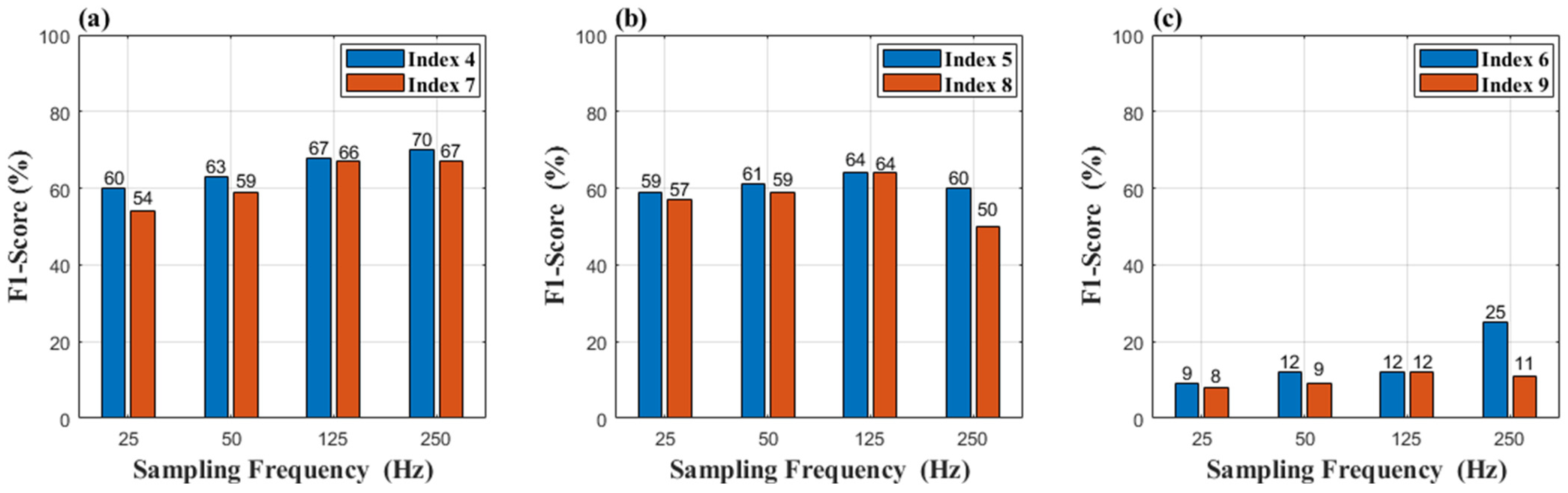
Figure 7 and Figure 8 are the results of a comparison between Group 2 and Group 3. In Figure 7a,b, the reference signal promotes the reconstruction of signals at a sampling rate of 25 Hz, and the F1-score increases by 6% in (a) and 2% in (b), respectively. In terms of the reconstruction error, reference signals play an important role to recover the details of the signals, as shown in Figure 8a,b. The RMSE of Group 2 has an obvious decrease compared to that of Group 3. However, the effectiveness of the reference signal is weaker in indices 6 and 9, as shown in Figure 8c, which indicates that signal V2 cannot provide enough information to recover the details of the signals (Leads I and II). We can be told by Figure 8 that signal “I” is the optimal option to be the reference signal.

Table 3. Experimental results of Index 10 and Index 1.

Sampling Frequency (Hz)	Index 10		Index 1
	RMSE (mV)	F1-Score (%)	RMSE (mV)	F1-Score (%)
25	0.17	63	0.10	84
50	0.15	81	0.08	89
125	0.12	83	0.05	90
250	0.08	81	0.04	95

shows the results of Index 1 and Index 10 (Group 4). Both the classification effectiveness and reconstruction error of the combination in Index 1 are superior to those in Group 4. At a sampling rate of 25 Hz, the combination in Index 1 obtained an F1-score of 84%, far more than that of Index 10. Although the RMSE of Index 10 decreases at the sampling rate of 125 Hz and 250 Hz, its F1-score also decreases. For this combination, the reason for this phenomenon is that the network does not perform well in some classes that include N, AF, RBBB, PAC, STD, and STE, as shown in

Table 4. Experimental result of the classification.

Type		N	AF	I-AVB	LBBB	RBBB	PAC	PVC	STD	STE	Average
F1-score	125 Hz	78	92	95	89	89	79	89	67	73	83
	250 Hz	75	87	95	93	86	78	91	60	66	81

. Although the details of the signals are better reconstructed, the main ECG features are not, such as the amplitude of R waves or T waves.

Figure 9 shows the comparison of the original signals, compressed signals, and reconstructed signals. In this figure, the left graph shows the signals of the lead II in indices 1 and 7. Another part shows the signals of the lead V2 in indices 1 and 7. To have a clear comparison, we overlaid the original signal on other waves. It can be seen clearly that the down-sampling operation eliminated the details of the red signals. Then, the details were reconstructed well by our network, shown as green and yellow waves in this figure. These green waves were better reconstructed compared with these yellow waves, especially the details of the signal, as shown by the red arrows in Figure 9. It indicates that the reference signal is helpful to recover the detail of the ECG.

To assess the impact of various down-sampling scales on power consumption. We measured the current of our device. The digital ammeter was KEITHLEY DMM7510, and the sampling frequency for the current measurement was 1 KHz. The measurement result is shown in

Table 5. The current measurement of the proposed method.

Sampling Frequency (Hz)	Current (mA)	Basic Current (mA)
25	6.07	5.85
50	6.23
125	6.46
250	7.13
500	7.83

. In addition, the diagram of the measuring current is shown in Figure 10. In Table 5, the current is averaged and measured within 1 h. The basic current refers to the BLE being in the broadcasting state and no data being transmitted. In this Table, the current decreases with the decrease in the sampling frequency.

We proposed a novel method to reduce data size while maintaining the features of ECG signals. Our method does not involve any complex computation used for compressing signals and has a good capability of reconstructing high-sampling-rate signals. There is an example of using the proposed method in our current project. In our project, the wearable ECG monitoring system was used to mainly detect atrial fibrillation (AF), and the detection of premature atrial contraction (PAC) and premature ventricular contraction (PVC) is of secondary importance. However, in our project, the working duration of the wearable device was short, and its battery could not be changed. Therefore, the objective of using the proposed method was to extend the working duration of the wearable device and maintain the detection capacity of the system for the main disease. When the wearable device has a high-level battery, the sampling frequency is 500 Hz. If the battery power becomes lower, the sampling frequency decreases to 250 Hz. In this state, the reconstructed signals may not have high enough quality to provide information on PAV and PVC but still can be used to detect AF from its RR intervals; therefore, the detection of the main disease can still be guaranteed. If the battery becomes lower, the sampling frequency decreases to 125 Hz or less. Finally, the working duration of the wearable device is extended and main disease detection is also guaranteed.

To our best knowledge, this work is the first attempt to use a deep learning network to reconstruct a signal and use a down-sampling operation to compress signals. Although the performance is in line with our expectations, it still has many limitations. The first limitation is the fixed sampling frequency. We plan to investigate the relationship between the sampling frequency and the ECG signal quality. When the ECG signal has good quality, the sampling frequency decreases. However, when the ECG signal has poor quality, the sampling frequency remains high to retain the detail of the signal. Moreover, we also plan to propose a more flexible structure for the network in our next work. The second limitation is that the quality of the reconstructed signal is highly relied on trained signals. We will expand the types of training data and improve the quality of training data. Meanwhile, we will validate the possibility that the network can remove noises when reconstructing signals.

5. Conclusions

In a wearable ECG monitoring device, the significant data size results in large energy consumption during wireless transmission and compression computation, thereby decreasing its monitoring duration. For our three-lead wearable ECG monitoring system, we developed a novel method to handle this problem. Our method utilizes a down-sampling operation to compress ECG signals and uses a proposed signal-referenced network to reconstruct the compressed signal. The down-sampling operation can be implemented in any wearable device and does not have any requirement for computing capability and memory. We validated the signal-referenced network on the CPSC 2018 database, and the experimental result shows an adequate performance of reconstructing high-sampling-rate signals. Our future objective is to develop a more flexible structure to support more sampling rates and reconstruct high-sampling-rate signals better.