Article

Study of Channel-Type Dynamic Weighing System for Goat Herds

1
College of Electronic Information Engineering, Inner Mongolia University, Hohhot 010021, China
2
Shanxi Wanli Technology Co., Ltd., Taiyuan 030032, China
3
State Key Laboratory of Reproductive Regulation and Breeding of Grassland Livestock, Hohhot 010020, China
4
School of Information Engineering, Inner Mongolia University of Science and Technology, Baotou 014010, China
*
Authors to whom correspondence should be addressed.
Electronics 2023, 12(7), 1715; https://doi.org/10.3390/electronics12071715
Submission received: 17 February 2023 / Revised: 28 March 2023 / Accepted: 31 March 2023 / Published: 4 April 2023
(This article belongs to the Topic Artificial Intelligence in Sensors)

Abstract

:
This paper proposes a design method for a channel-type sheep dynamic weighing system to address the current problems encountered by pastoralists at home and abroad, such as time-consuming sheep weighing, difficulties with data collection, and management of the stress response in sheep. The complete system includes a hardware structure, dynamic characteristics, and a Kalman-aggregate empirical modal decomposition algorithm (Kalman-EEMD algorithm) model for dynamic data processing. The noise suppression effects of the Kalman filter, the empirical modal decomposition (EMD), and the ensemble empirical modal decomposition (EEMD) algorithms are discussed for practical applications. Field tests showed that the Kalman-EEMD algorithm model has the advantages of high accuracy, efficiency, and reliability. The maximum error between the actual weight of the goats and the measured value in the experiments was 1.0%, with an average error as low as 0.40% and a maximum pass time of 2 s for a single goat. This meets the needs for weighing accuracy and goat flock weighing rates.

1. Introduction

With the development and progress of Chinese society, people’s requirements for clothing, food, housing, and transport are increasing. To meet the huge demand for beef and goat meat, the development of animal husbandry is becoming increasingly large-scale and refined [1]. Through high-precision sensors, herdsmen can correlate disease, nutrition, reproduction, and production with the weight, water intake, and exercise levels of their goats and then combine this with automated equipment to form a smart livestock platform for refined breeding and scientific management [2]. In livestock production, livestock farmers can obtain the fat condition and growth pattern of their livestock in real-time through weight changes so that they can improve their feeding methods in real-time and increase the meat production rate, fleece production rate, and reproduction rate of their livestock. To achieve this, it is necessary to measure the weight of their livestock on a regular basis [3].
At present, most of the weighing scales in the domestic market are made by adding a fence to the bench scale, which not only restricts the action of the goats but also requires manual counting and recording of ear tags and weight information, which is inefficient due to the amount of required manual labor; this can also be inaccurate. Dynamic scales squeeze the goats into a small space so that they cannot move for the measurements, which is more efficient but can be slow and costly to maintain [4,5,6]. Both of these methods can frighten the goats, lowering their immunity and increasing the incidence of disease, which is not conducive to healthy goat growth. For the dynamic weighing of livestock, Y. Wang used artificial neural network techniques to associate a large number of physical features extracted from walking images with the live weight of pigs, with an average relative error of around 3% [7]. X. Song et al. also proposed quantifying the error in weight prediction using morphological traits automatically measured by a 3D vision system [8]. In 2019, Wang Kui et al. designed a dynamic goat-weighing herding system to compare the EMD algorithm and the mean algorithm, which yielded an average error of 1.1% for the EMD algorithm and 2.7% for the mean algorithm within the same elapsed time of 8.4 s. However, the different lengths of wool (fleece) from seasonal sheep cover the sheep’s body to varying degrees, altering the size of the sheep’s body surface area and rendering weight measurement using image processing methods unsuitable. The method of Wang Kui et al. is too time-consuming and has a high degree of error in weighing a single goat.
Based on the current development of dynamic weighing, and the problems encountered by domestic and foreign herders, such as time-consuming sheep weighing and inaccurate weight data that are difficult to collect, this paper proposes a channel-type sheep dynamic weighing system. The STM32 chip is used as the console to collect and calculate the weight data, which are displayed in real-time on a touch screen. The dual storage mechanism of offline exporting by an SD card module and uploading to server storage by a WiFi module ensures data security. A mobile phone front-end and a computer front-end are used to display the results in real-time. The practical test results showed that the system is stable and reliable, with high accuracy and speed in dynamic weighing and that it can accurately record the growth and weight changes of livestock in real-time.

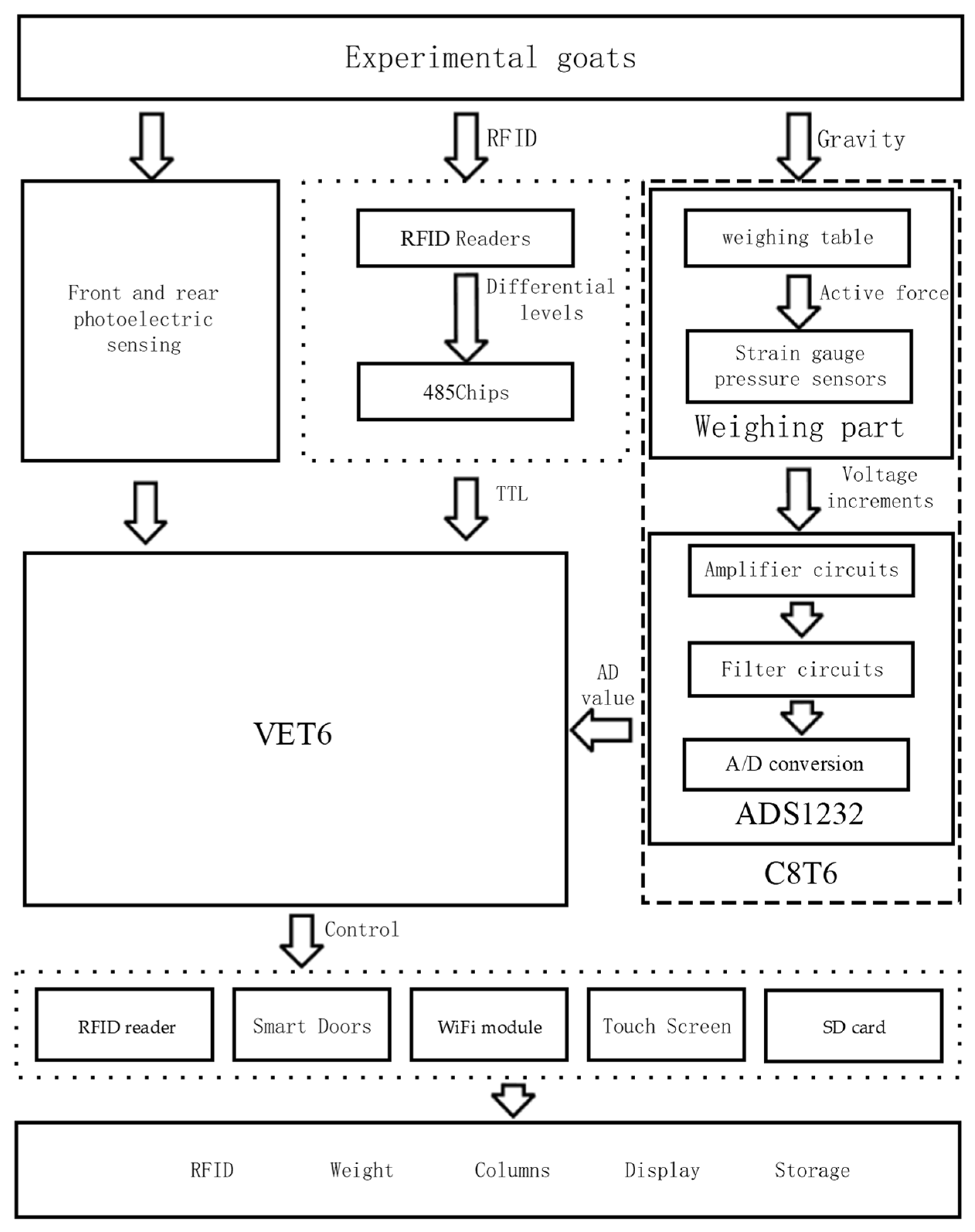
2. Principles of Operation and System Structure of the Channel-Type Flock Dynamic Weighing System

2.1. Working Principles of the Channel-Type Sheep Dynamic Weighing System

The basic workflow of the channel-type goat-weighing system begins when the goat steps into the weighing platform through the channel section. Pressure is applied to the pressure transducer, and the strain gauges in the pressure transducer are deformed, and their resistance value changes accordingly. This is then connected to a bridge, where the change in resistance can be indirectly measured by measuring the change in bridge voltage to obtain the magnitude of the external force applied. The bridge output is connected to an analog-to-digital conversion circuit. When working, the bridge will obtain the electrical signal into the analog-to-digital conversion chip, and the analog-to-digital conversion chip will amplify and filter the electrical signal and then convert it into a digital signal to the master control. The master control on the digital signal processing obtains the weight, while the RFID reader reads the goat’s ear tag number and transmits it to the master control. The master control then divides the flock by the data obtained and displays and stores the information obtained on the ear tag, the weight, and the division of the flock. The workflow diagram of the channel-type goat dynamic weighing system is shown in Figure 1.

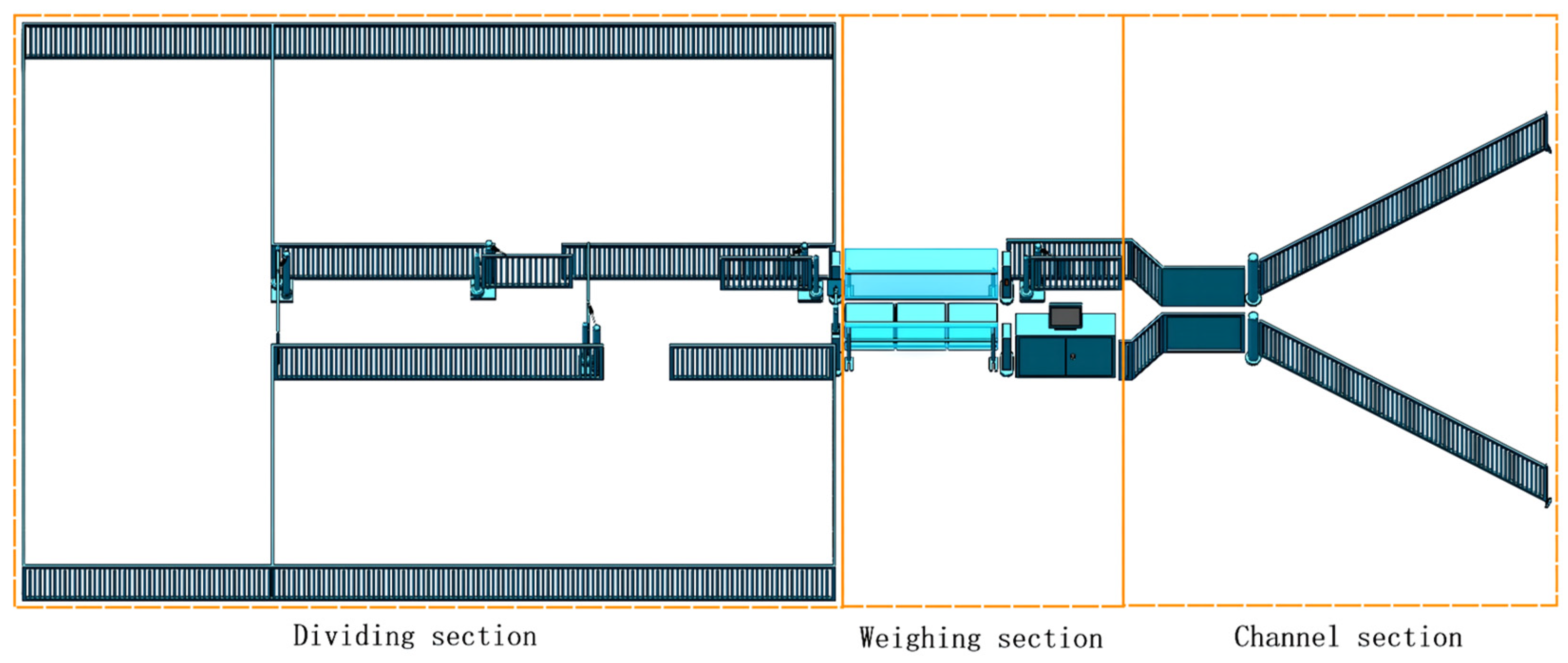
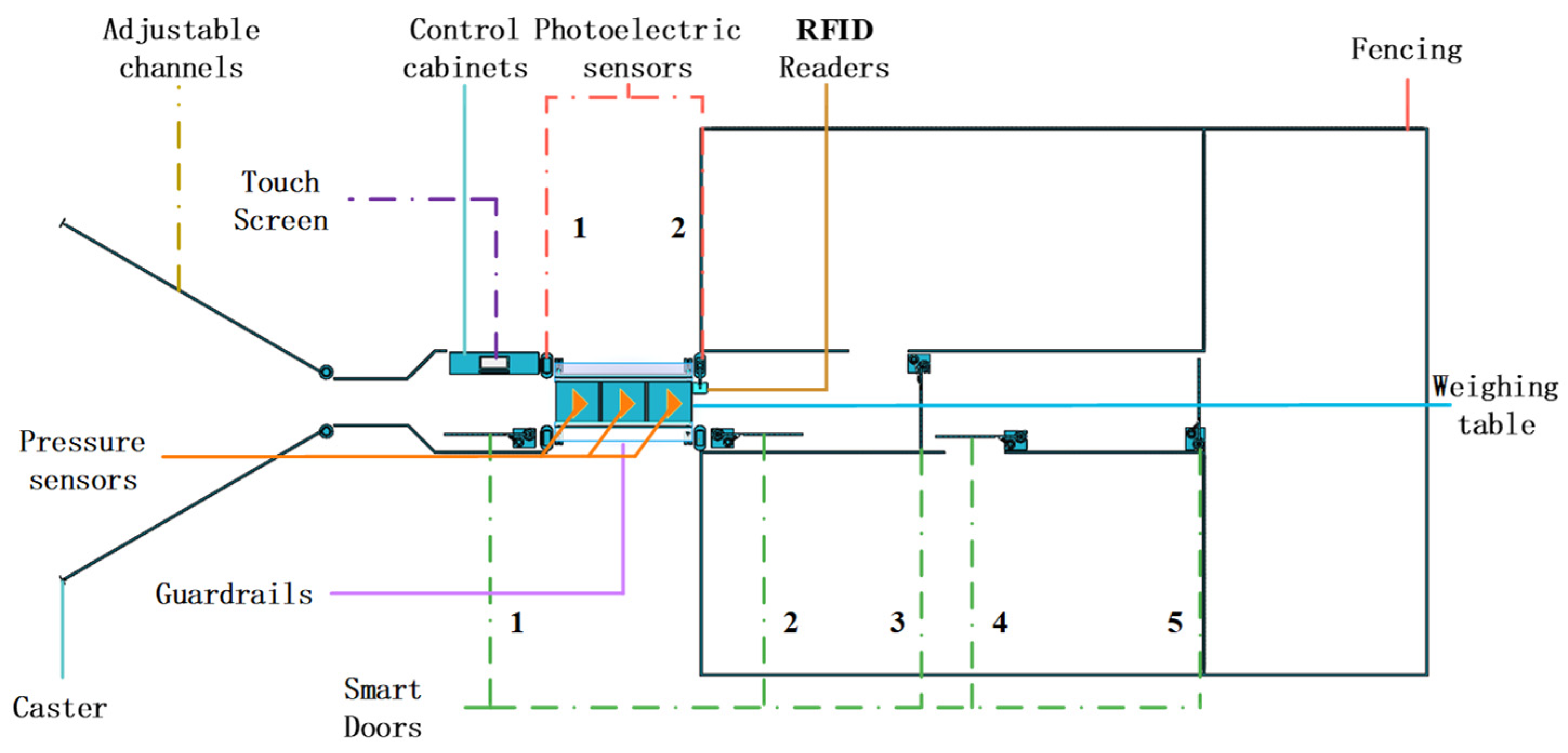
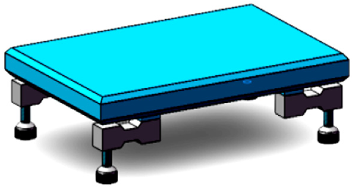
2.2. Channel-Type Flock Dynamic Weighing System Construction

The system architecture is shown in Figure 2, with an overall choice of three weighing body splicing structures, with a single weighing body size set at (60 × 45) cm according to the body length and width of the goat. The main functional structure consists of the channel section, the weighing section, and the dividing section.
The structure of the sensor is shown in Figure 3. The front end of the channel section is set up as a flared shape with castors, and the rear end of the proximity weighing section is set up as a linear structure channel with adjustable width. The weighing section uses an AVIC L6G pressure sensor for pressure signal collection, a 24-bit high-precision analog-to-digital conversion unit ADS1232 for data conversion, an Omron photoelectric sensor to obtain the real-time position of the sheep, and a RFID reader for ear tag reading. Actuators and electric actuators make up the smart gate drive module, the human–machine interface is realized by a touch screen, and the fence and the smart gate are controlled by the drive module to make up the fencing section.

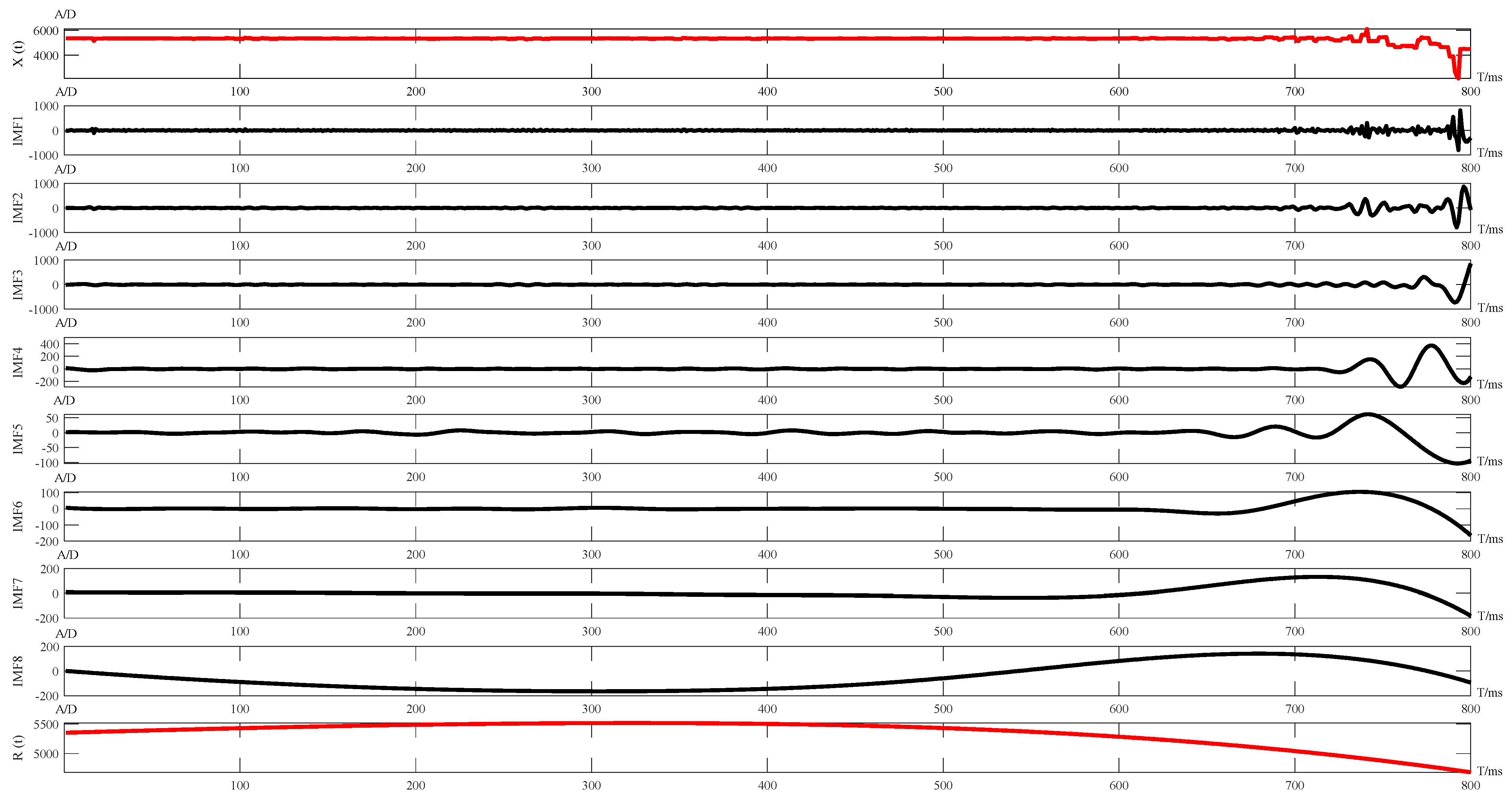
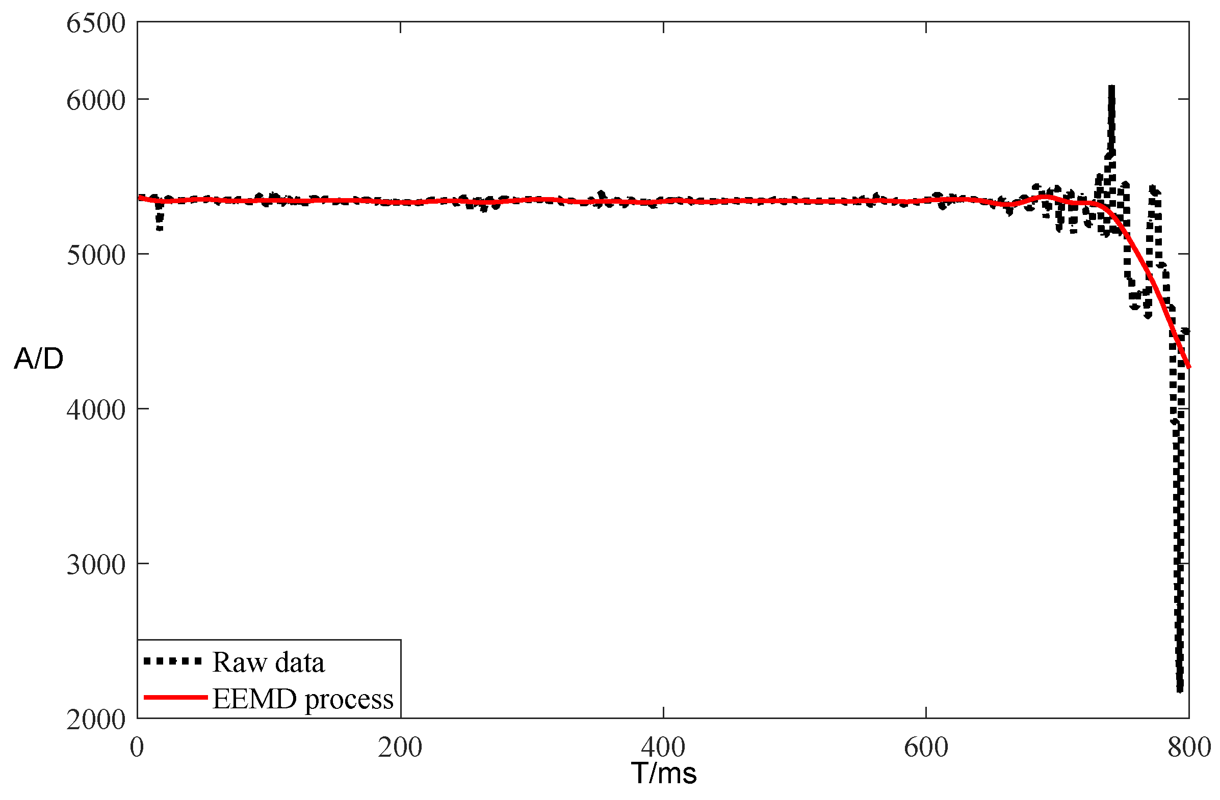
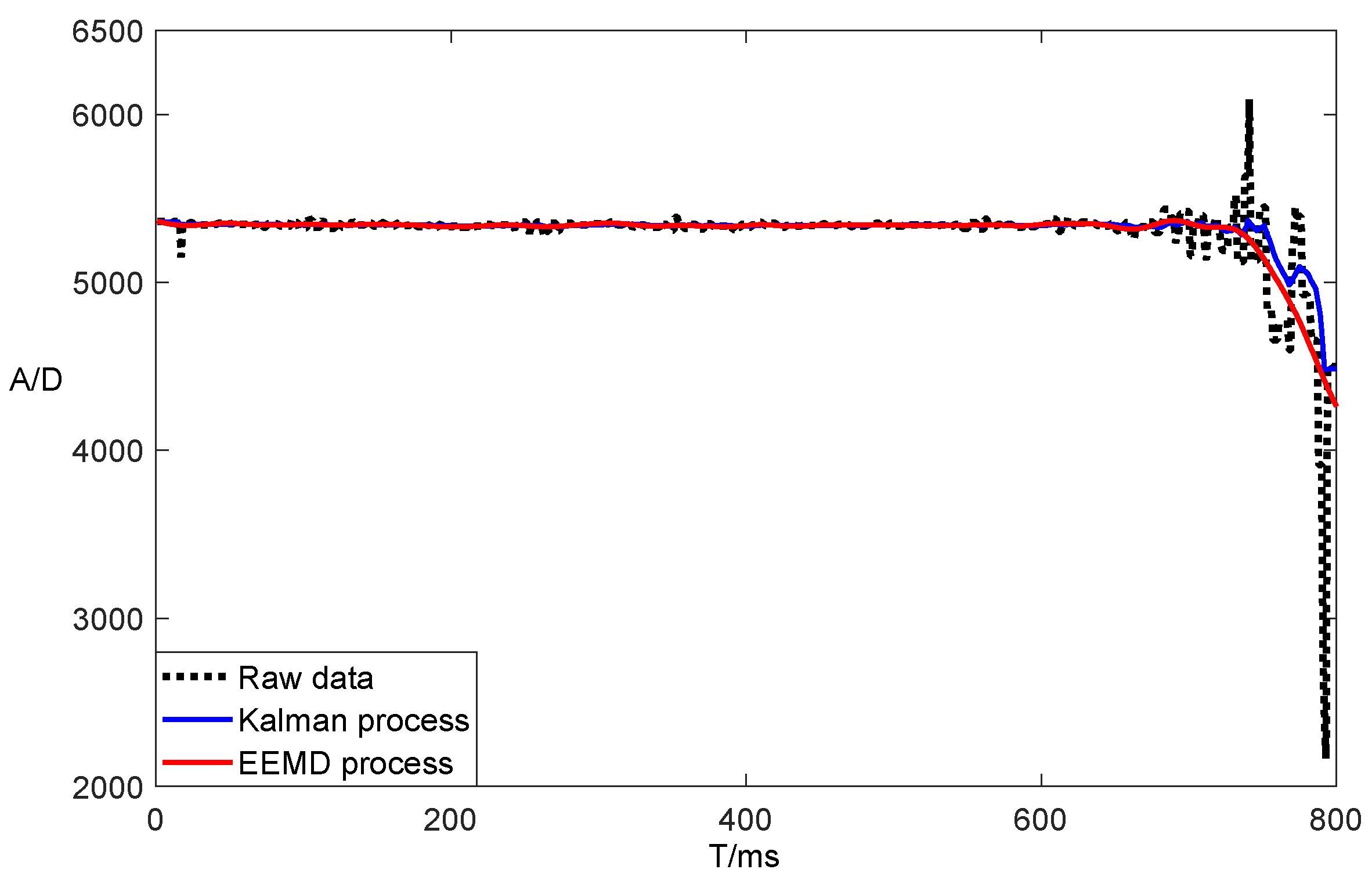
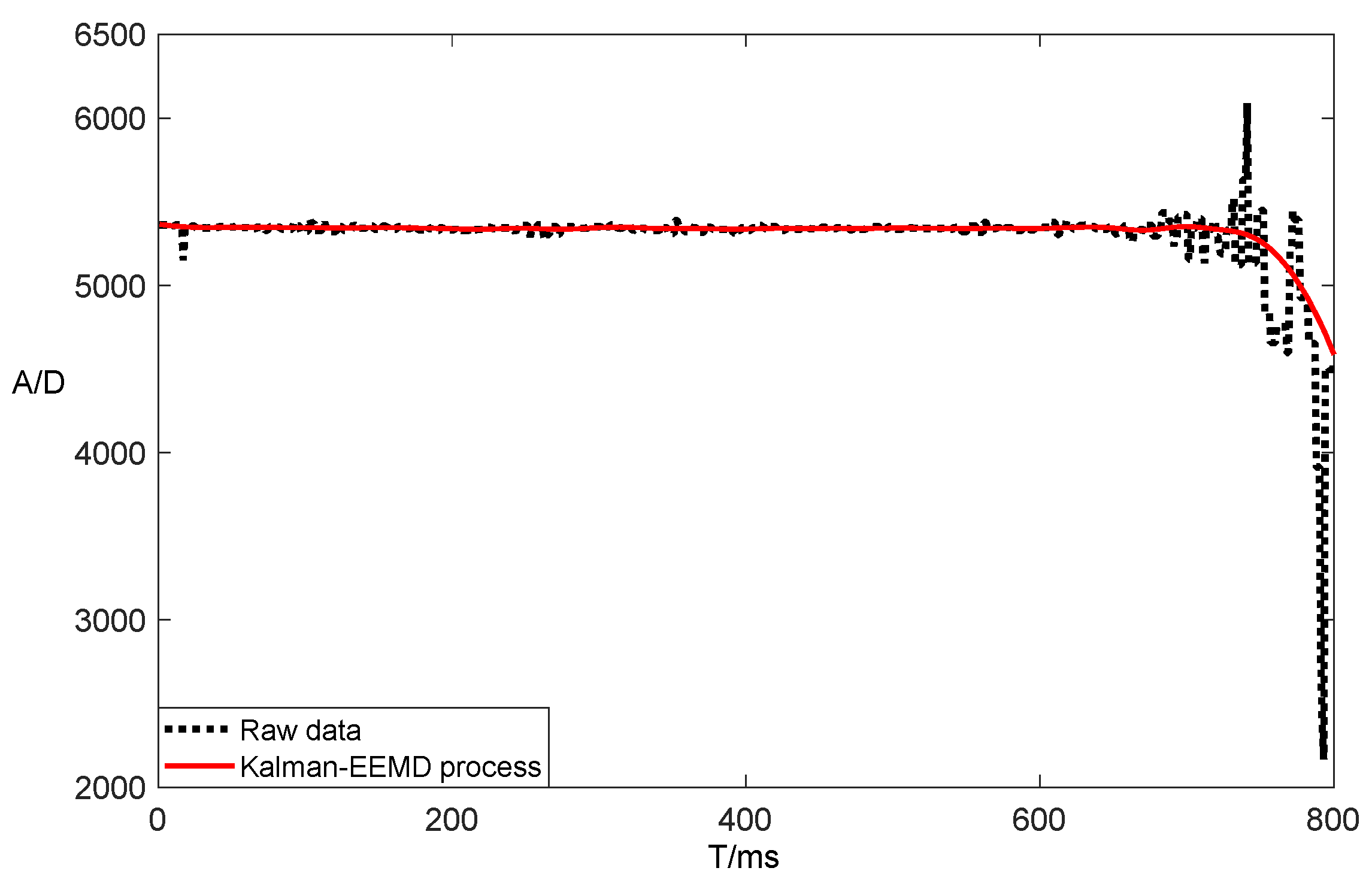
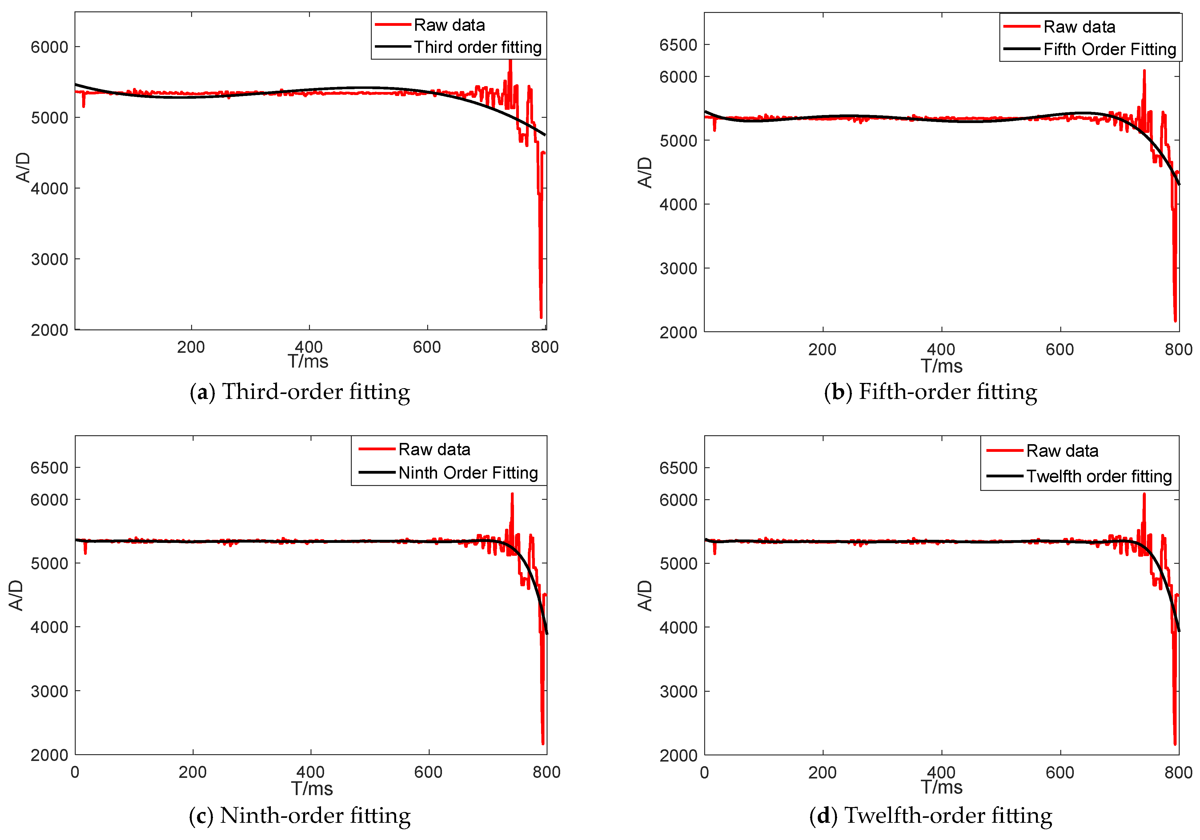
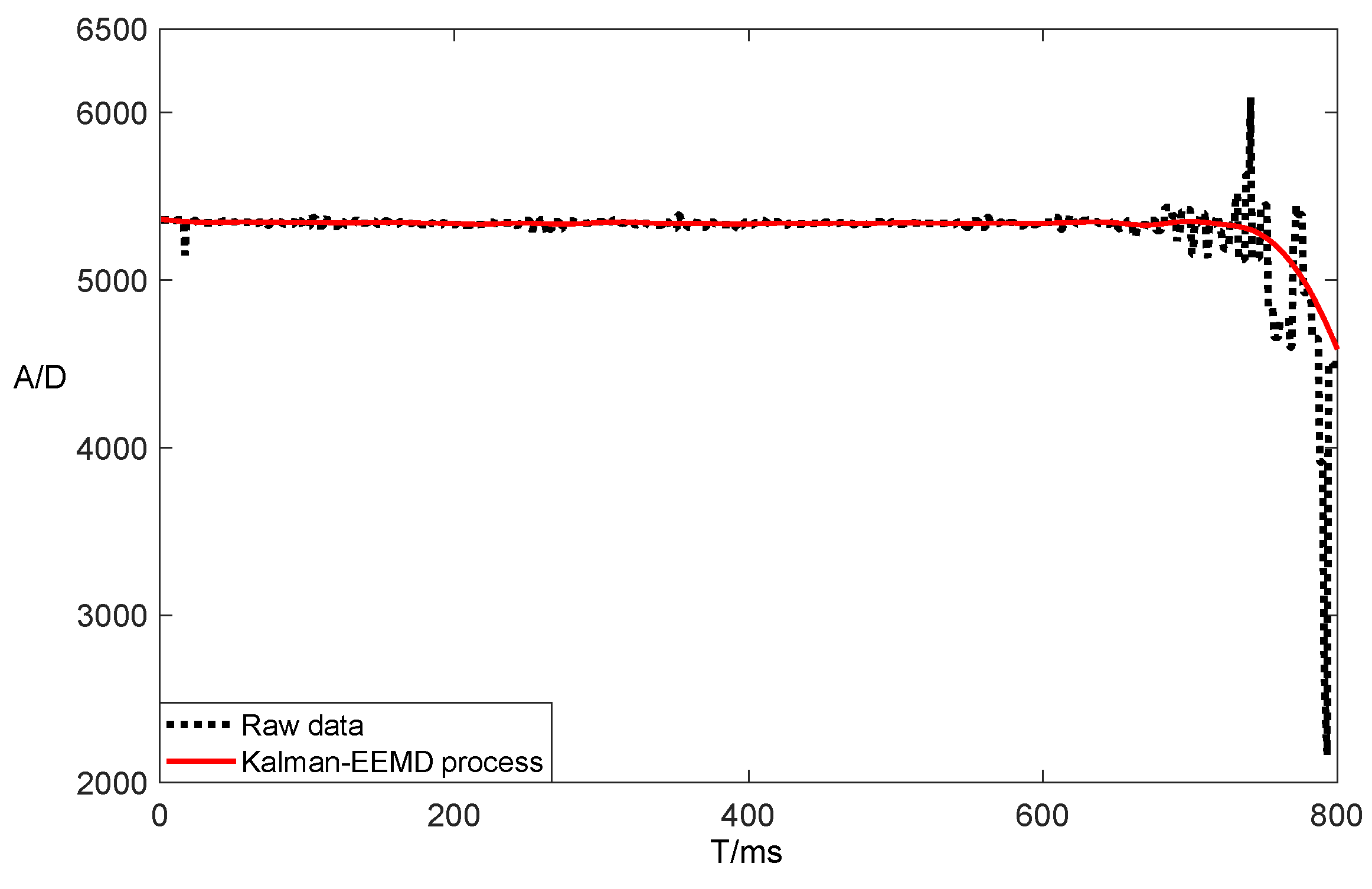
3. Algorithm Design for the Weighing Section

As the goat enters the weighing section, the front door closes, and the rear door opens. The goat passes through the three weighing bodies in the weighing section in turn, and the data changes after passing through the three weighing bodies are collected and collated, as shown in Figure 4.
When the goat steps on the weighing body, in the process of moving forward, there is a certain impact on the body, which makes the pressure on the weighing body unstable, and the data obtained change accordingly. To ensure that the algorithm used in the weighing part fits the hardware architecture of this system and improves the measurement accuracy, and analysis of the data obtained from the sensors was performed through a simulation system to find a suitable algorithm. The model used for the tests was a single weighing body with a four pressure sensors structure, as shown in Figure 5.
Under ideal conditions, the change in data produced by the goat stepping into the weighing body to leaving it gently is shown in Figure 6, which divides the whole action into three stages: on the scale, in the scale, and off the scale.
In Figure 6, S_1, S_2, S_3, and S_4, the AD values obtained by the four sensors of the weighing body are shown, and S_sum is the sum of the AD values obtained by the four sensors. To summarize:
(1) Severe spike disturbances occurred in the data when the goats were weighed on and off the scales.
(2) The data fluctuated when goats made movements on the weighing body.
(3) Each goat will cause slight fluctuations when traveling smoothly on the weighing body.
(4) As the goat travels on the weighing body, the S_1, S_2, S_3, and S_4 data changed significantly, and the sum S_sum could ideally be considered constant.
As in Figure 6, if valid data are retained, the noise jitter, data spikes on the rising and falling edges, and data fluctuations generated by the action need to be removed from the part marked by the dashed line.
A relatively small single-in, single-out sliding window dataset was created in the sub-controller C8T6 program to remove the data spikes generated when the goat was weighed. The structure of the data group used to solve this data spike problem is shown in Figure 7, and the effect of removing the weighing spike is shown in Figure 8.
Various data processing algorithms were simulated by a simulation system, and we found that the Kalman filter and EEMD algorithms were the best for spike jitter [9].
Using the first-order Kalman filter algorithm for data processing, the Kalman filter process was divided into two main steps, namely, the prediction phase and the correction phase. Prediction phase: An initial optimal estimate of the system state variables for the current round was made, and then the system covariance matrix was calculated for the current round of predictions. Correction phase: We calculated the Kalman gain, then corrected the a priori estimate using the residuals of the observed and predicted values, and finally updated the covariance matrix to provide the system with a basis for the next round of calculations, as shown in Figure 9.
Kalman filter time update equation:
X k = A X k 1 + B u k 1
From the optimal estimate of the system state variable at moment k − 1, the system prediction at moment k was calculated. Xk is the current state optimal estimate predicted using the k − 1 moments, A is the coefficient matrix under the previous state Xk−1, B is the control matrix, and u is the control quantity. When dealing with one-dimensional data, A = 1, B = 0, and uk−1 = 0; that is, Xk = Xk−1.
P k = A P k 1 A T + Q
The system covariance at moment k was predicted from the system covariance at moment k − 1, where Pk is the system noise covariance matrix at moment k, Pk−1 is the system noise covariance matrix at previous moment k − 1, and Q is the covariance of the system process noise.
Kalman filter state update equation:
K k = P k H T ( H P k H T + R ) 1
We calculated the Kalman gain Kk at moment k. H is the observation matrix of the object, and R is the covariance matrix of the observation noise, which needs to be derived experimentally during the commissioning process. When dealing with one-dimensional data, H = 1.
X k = X k + K k ( Z k H X k )
The optimal value of the state variable at moment k was calculated from the predicted value of the state variable and the observed value of the system, Zk object.
P k = ( I K k H ) P k
We updated the covariance matrix of the system process noise for use in the next iteration, where I is the unit matrix. Since the first Kalman filter operation was performed without Xk, the first value of the dataset obtained after the operation could not be used; to solve this problem, the second number of the array was assigned to the first one after the operation.
Based on the testing with Q set to 0.01 and R set to 0.05, the experimental results are shown in Figure 10, where the black dashed line represents the raw data, and the red line is the filtered data. As shown in the figure, the use of the first-order Kalman filter effectively removed the jitter in the horizontal section, although there was still minor jitter in the processing of the spiky data section, although the filtering effect was significant.
The empirical mode decomposition (EMD) method is an adaptive time-frequency localization analysis method proposed by Huang et al. [10,11,12]. Its basic functions are generated automatically, and it can decompose the raw signal into multiple intrinsic mode function IMF components and a residual, with each IMF representing the variation of the raw signal at different frequencies, while the residual reflects the slowly changing amount of data in the signal. The EMD algorithm steps are shown in Figure 11.
Assuming the raw signal x(t), we found all local maxima and minima in x(t) and used the cubic spline interpolation to fit the local maxima to the upper envelope emax(t) and the local minima to the lower envelope emin(t).
The mean value envelope m(t) was obtained by calculating the average of the upper and lower envelopes at each time point:
m ( t ) = 1 2 [ e m a x ( t ) + e m i n ( t ) ]
The raw signal was subtracted from the mean envelope to obtain h(t):
h ( t ) = x ( t ) m ( t )
At the end of this step, we determined if h(t) satisfied the condition of being an intrinsic modal function IMF [13,14,15]. If h(t) satisfied the condition, h(t) was considered an intrinsic modal function C(t) of the raw signal. The conditions for an IMF of a modal function were met:
(1) The total number of extremes in the whole set of integers was the same as the number of crossing zeros or differed by 1.
(2) The mean envelope of the upper and lower envelopes was zero for any given time period, and the entire waveform was locally symmetrical.
If h(t) did not satisfy the condition, we used the current h(t) as the new raw signal. This was repeated until the condition of the intrinsic modal function IMF was satisfied.
r ( t ) = x ( t ) h ( t )
R(t) is the residual component corresponding to the current intrinsic mode function IMF. r(t) was treated as the new raw signal, and the above steps are repeated until the EMD decomposition process ended when the intrinsic mode function IMF could no longer be decomposed.
The sum of all intrinsic modal functions IMF and the remaining residual components was the raw signal x(t):
x ( t ) = k = 1 n C k ( t ) + r n ( t )
CK(t) is the intrinsic modal function component, and rn(t) is the residual component, which generally represents the average trend and is a constant or monotonic series. The raw signal EMD algorithm was decomposed as in Figure 12.
As in Figure 12, there was multiple modal mixing of the IMF components of the raw signal, i.e., one IMF contained feature components at different time scales, and the conditions under which the EMD iterative process should be stopped lack criteria [16,17]. To solve the modal mixing phenomenon, Huang introduced a uniformly distributed frequency of 0-mean white noise into the raw signal to be analyzed so that signals of different time scales were automatically separated to their corresponding reference scales, which is the ensemble empirical mode decomposition (EEMD) algorithm, and the steps of the EEMD algorithm are shown in Figure 13 [18,19].
We first set the overall average number of times M. A standard normally distributed white noise ni(t) was added to the raw data to form a new signal.
x i ( t ) = x ( t ) + n i ( t )
Xi(t) is the signal after the additional noise of the i-th trial, and ni(t) is the white noise sequence added in the i-th trial [20]. The EMD decomposition of the signal after the addition of white noise was then performed to obtain
c 1 , j ( t )   c 2 , j ( t ) c M , j ( t ) , j = 1 , 2 , J
Ci,j(t) is the j-th IMF obtained by decomposing after the i-th addition of white noise and r i,j(t) is the residual function (i = 1, 2, 3, …, M). We repeated the above steps M times to repeatedly decompose the set of IMFs obtained by adding white noise signals with different amplitudes.
x i ( t ) = j = 1 J c i , j ( t ) + r i , j ( t )
Finally, the above corresponding IMFs were pooled and averaged to obtain the final IMF after EEMD decomposition, i.e.,
c j ( t ) = 1 M i = 1 M c i , j ( t )
Cj(t) is the j-th IMF of the EEMD decomposition (i = 1, 2, 3, …, M; j = 1, 2, 3, …, J). The EEMD decomposition of the raw signal is shown in Figure 14.
As shown in Figure 14, compared with the EMD algorithm, after adding white noise, the first-order IMF component to the eighth-order IMF component all contained only one frequency component, and there was no modal mixing phenomenon, so the EEMD algorithm was selected as the algorithm for sub-control. After several experiments, the EEMD algorithm had the best effect on the raw data when the standard deviation of the white noise was 0.5, and the number of noises was 100, as shown in Figure 15, where the black dashed line is the raw data and the red line is the data after processing by the EEMD algorithm.
As shown in Figure 16, the elimination of jitter in the horizontal part of the EEMD algorithm was largely not different from the effect of the first-order Kalman filter, and the processing of spiky data by the EEMD algorithm was much smoother, with almost no fluctuations [21,22]. The black dashed line in Figure 16 is the raw data, the blue line is the data after Kalman filtering, and the red line is the data after processing by the EEMD algorithm. This figure shows that for the processing of spiky data, the EEMD algorithm had the best processing effect, and the EEMD algorithm was finally selected as the initial filtering algorithm.
The raw data were processed by the EEMD algorithm, as shown in Figure 15. The red line is the processed data, and it started to fluctuate at the horizontal coordinate 600. In order to enhance the filtering effect, the Kalman filter was selected as the main control for the secondary filtering of the data. The processing effect is shown in Figure 17, where the red solid line shows the data processed by the Kalman-EEMD algorithm, and the black dashed line shows the change in the raw data. In comparison with Figure 10 and Figure 15, the Kalman-EEMD algorithm model had a better filtering effect than the filtering algorithm alone.
A polynomial fit was used to fit the raw data, and the fitting results are shown in Figure 18, with the red line representing the raw data and the black line the fitted data. The third-order fit and fifth-order fit in the figure are poor, and the fit graph appears to overshoot after exceeding the ninth-order. Through experimentation, the ninth-order fit was found to be the best. The results were compared with the Kalman-EEMD filtering effect, and the results are shown in Figure 19.
In Figure 19, the black line is the data processed by the Kalman-EEMD filtering algorithm, and the red line is the data after the ninth-order fit. The fitting function is
f ( x ) = p 1 × x 9 + p 2 × x 8 + p 3 × x 7 + p 4 × x 6 + p 5 × x 5 + p 6 × x 4 + p 7 × x 3 + p 8 × x 2 + p 9 × x + p 10
where p1 = −1.54 × 10⁻²⁰, p2 = 4.935 × 10⁻¹⁷, p3 = −6.615 × 10⁻¹⁴, p4 = 4.81 × 10⁻¹¹, p5 = −2.057 × 10⁻⁸, p6 = 5.246 × 10⁻⁶, p7 = −0.0007712, p8 = 0.05986, p9 = −2.08, and p10 = 5367. In comparison, the Kalman-EEMD filtering algorithm in the horizontal region achieved the desired filtering effect; the Kalman-EEMD filtering algorithm was better than the ninth-order best fit because the ninth-order fit showed an overshoot at the horizontal coordinate 700.
After the experiments, the sub-controller used the EEMD algorithm for the initial processing of the valid dataset intercepted by the sliding window, and the main control used the Kalman filter for the secondary processing. A stepwise processing method was used for data processing, and a Kalman-EEMD algorithm model was constructed, which guaranteed the operation rate and accuracy, and achieved the optimal choice of dynamic weighing algorithm.

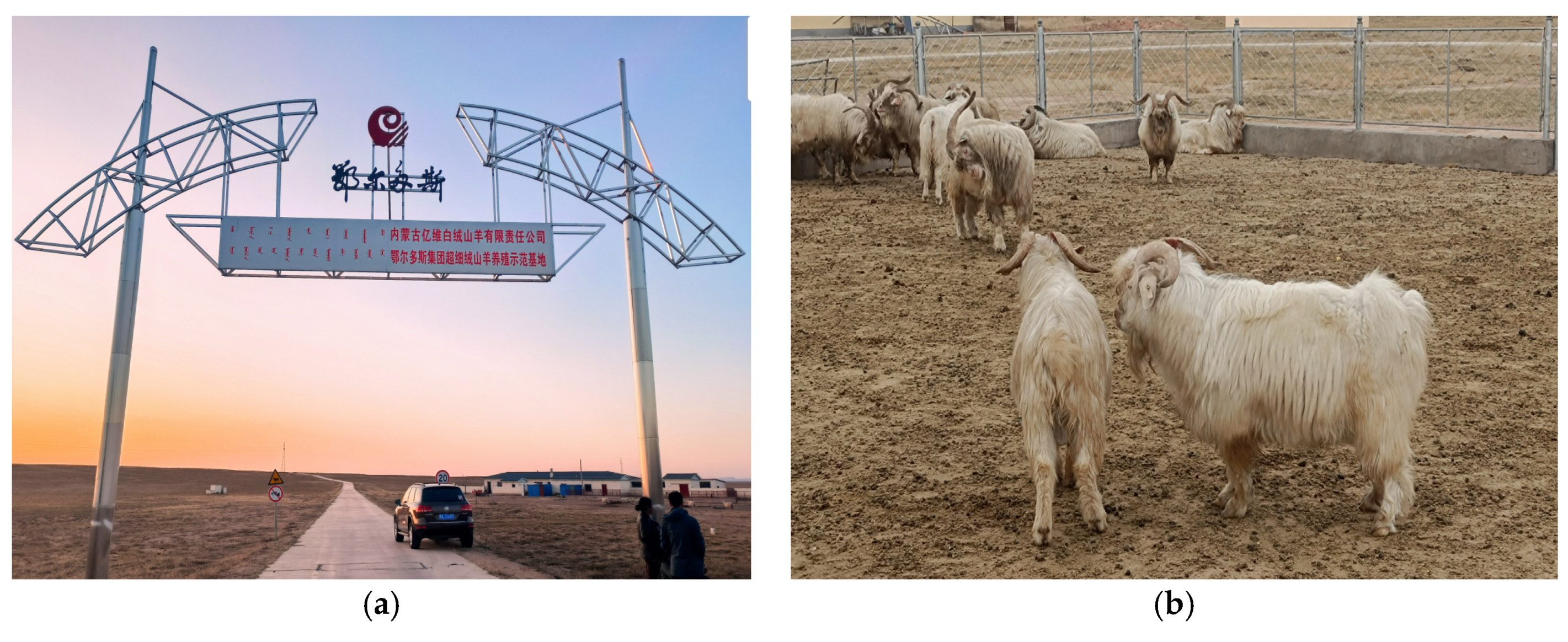
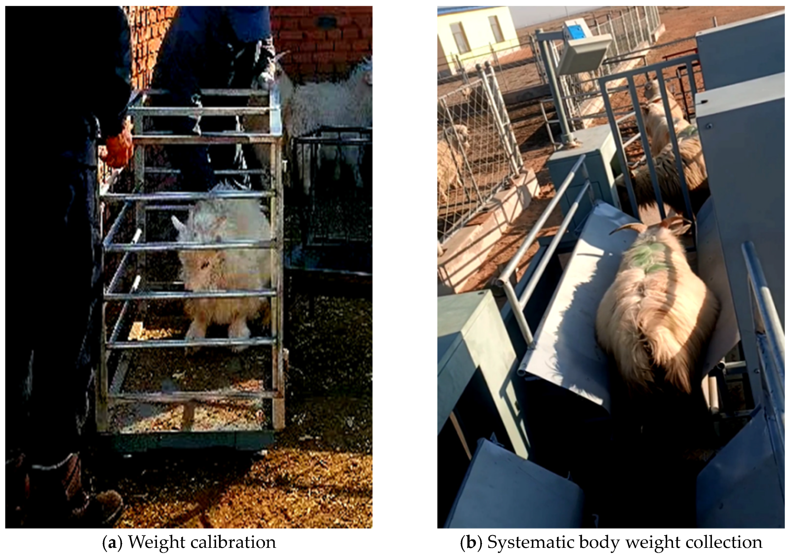
4. Field Experiments and Data Analysis of the System

In Figure 20a,b, in order to test the field effect of the whole system, an experiment was conducted on 13 December 2021 at the Sanbei goat farm in Erdos, Inner Mongolia. A flock of 30 Albas white cashmere goats was selected for testing in the experiment. The actual weight of the goats and the corresponding ear tag number were recorded before the test, and then the flock was made to pass through the whole system three times.
The experimental site is shown in Figure 21a,b. During the experiments, the sorting thresholds were adjusted on-site using the touch screen human–machine interface, with those weighing more than 45 kg entering area A, those weighing between 35 and 45 kg entering area B, and those weighing less than 35 kg entering area C. The system achieved intelligent sorting according to the set thresholds.
(1) First experimental result:
(2) Second experimental result:
(3) Third experimental result:
There were 30 sets of data in the experiment, as shown in Figure 22. In the first experiment, 16 sets of data had an error of 0, and only 1 set of data had an error of 1%, with an average error of about 0.32%. In the second experiment, as shown in Figure 23, seven sets of data had an error of 0, and two sets of data had an error of 1%, with an average error of 0.48%. In the third experiment, as shown in Figure 24, eight sets of data had an error of 0, and two sets of data had an error of 1%, with an average error of 0.40%. The total error was 0.40%.
The results of the experiment are shown in Table 1.
As can be seen from the above graphs, the field trial achieved the expected results. With improved weighing accuracy, the weighing rate of the sheep is guaranteed to be intelligent and scalable, which will provide a reliable data basis for the development of precise and ecologically sound animal husbandry. The minimum error between the actual weight and the measured value in the experiment was 0, the maximum error was 1.0%, and the average error was as low as 0.4%, demonstrating high accuracy. A total of 30 sheep passed through the whole system in about 54 s. The shortest time for a single sheep to pass through was 1.5 s, the longest time was 2 s, and the average time was 1.8 s.

5. Conclusions

Large-scale animal husbandry is the mainstream direction of the current modern development of animal husbandry. In order to realize refined breeding and scientific management, a channel-type sheep dynamic weighing system was designed. Using STM32F103VET6 as the main control and STM32F103C8T6 as the sub-control, it acquired weight data, read RFID ear tags, controlled electric pushers to open and close the door, and the touch screen displayed and stored the current goat ear tag number, weight data, flock information, and total flock weight. Using the Kalman-EEMD algorithm model for data processing in field trials, the designed system ensured weighing accuracy and improved the efficiency of goat weighing, achieving an intelligent flock-splitting effect with no constraints on goat action and no stress reaction. It improved the weighing rate and weighing accuracy, and it can be promoted and applied in the development of large-scale livestock farming.

Author Contributions

Conceptualization, Z.H. and D.H.; methodology, Z.H. and D.H.; software, Z.H., J.X. and K.W.; validation, Z.H., K.W. and J.C.; formal analysis, Z.H. and H.D.; investigation, Z.H. and K.W.; resources, Z.H., D.H. and J.C.; data curation, Z.H. and Y.G.; writing—original draft preparation, Z.H.; writing—review and editing, Z.H., D.H. and Y.G.; visualization, Z.H., J.X. and H.D.; supervision, D.H., Y.G. and J.C.; project administration, Z.H. and D.H.; funding acquisition, D.H. All authors have read and agreed to the published version of the manuscript.

Funding

This research was funded by the Major Science and Technology Projects of Inner Mongolia Autonomous Region under grant number 2021ZD0019-4.

Data Availability Statement

Some or all of the data, models, or code generated or used during the study are available from the corresponding author by request (raw data, site data, algorithm model).

Acknowledgments

This work was supported by the major science and technology projects of Inner Mongolia Autonomous Region under GM 2021ZD0019-4. The authors would like to thank the funding bodies for their financial support.

Conflicts of Interest

The authors declare no conflict of interest.

References

  1. Cappai, M.; Rubiu, N.; Nieddu, G.; Bitti, M.; Pinna, W. Analysis of fieldwork activities during milk production recording in dairy ewes by means of individual ear tag (ET) alone or plus RFID based electronic identification (EID). Comput. Electron. Agric. 2018, 144, 324–328. [Google Scholar] [CrossRef]
  2. Niedźwiecki, M.; Wasilewski, A. Application of adaptive filtering to dynamic weighing of vehicles. Control Eng. Pract. 1996, 4, 635–644. [Google Scholar] [CrossRef]
  3. Huang, N.E.; Shen, Z.; Long, S.R.; Wu, M.C.; Shih, H.H.; Zheng, Q.; Yen, N.-C.; Tung, C.C.; Liu, H.H. The empirical mode decomposition and the Hilbert spectrum for nonlinear and non-stationary time series analysis. Proc. R. Soc. 1998, 454, 903–995. [Google Scholar] [CrossRef]
  4. González-García, E.; Alhamada, M.; Nascimento, H.; Portes, D.; Bonnafe, G.; Allain, C.; Llach, I.; Hassoun, P.; Gautier, J.; Parisot, S. Measuring liveweight changes in lactating dairy ewes with an automated walk-over-weighing system. J. Dairy Sci. 2021, 104, 5675–5688. [Google Scholar] [CrossRef]
  5. Mendoza-Lugo, M.A.; Morales-Nápoles, O.; Delgado-Hernández, D.J. A Non-parametric Bayesian Network for multivariate probabilistic modelling of Weigh-in-Motion System Data. Transp. Res. Interdiscip. Perspect. 2022, 13, 100552. [Google Scholar] [CrossRef]
  6. Polat, E.S.; Çağlayan, T.; Garip, M.; Coşkun, B. Improving mobile sheep walk-over weighing system designed for quick, easy and accurate evaluation of herds’ status in field. Curr. Opin. Biotechnol. 2013, 24, S28. [Google Scholar] [CrossRef]
  7. Wang, Y.; Yang, W.; Winter, P.; Walker, L. Walk-through weighing of pigs using machine vision and an artificial neural network. Biosyst. Eng. 2008, 100, 117–125. [Google Scholar] [CrossRef]
  8. Song, X.; Bokkers, E.; van der Tol, P.; Koerkamp, P.G.; van Mourik, S. Automated body weight prediction of dairy cows using 3-dimensional vision. J. Dairy Sci. 2018, 101, 4448–4459. [Google Scholar] [CrossRef] [Green Version]
  9. Jiang, L.; Liu, N. Correcting noisy dynamic mode decomposition with Kalman filters. J. Comput. Phys. 2022, 461, 111175. [Google Scholar] [CrossRef]
  10. Peng, Z.; Tse, P.W.; Chu, F. An improved Hilbert–Huang transform and its application in vibration signal analysis. J. Sound Vib. 2005, 286, 187–205. [Google Scholar] [CrossRef]
  11. Liu, B.; Riemenschneider, S.; Xu, Y. Gearbox fault diagnosis using empirical mode decomposition and Hilbert spectrum. Mech. Syst. Signal Process. 2006, 20, 718–734. [Google Scholar] [CrossRef]
  12. Bin, G.; Gao, J.; Li, X.; Dhillon, B. Early fault diagnosis of rotating machinery based on wavelet packets—Empirical mode decomposition feature extraction and neural network. Mech. Syst. Signal Process. 2012, 27, 696–711. [Google Scholar] [CrossRef]
  13. Junsheng, C.; Dejie, Y.; Yu, Y. A fault diagnosis approach for roller bearings based on EMD method and AR model. Mech. Syst. Signal Process. 2006, 20, 350–362. [Google Scholar] [CrossRef]
  14. Bian, K.; Wu, Z. Data-based model with EMD and a new model selection criterion for dam health monitoring. Eng. Struct. 2022, 260, 114171. [Google Scholar] [CrossRef]
  15. Zou, S.; Qiu, T.; Huang, P.; Bai, X.; Liu, C. Constructing Multi-scale Entropy Based on the Empirical Mode Decomposition(EMD) and its Application in Recognizing Driving Fatigue. J. Neurosci. Methods 2020, 341, 108691. [Google Scholar] [CrossRef]
  16. Lin, D.-C.; Guo, Z.-L.; An, F.-P.; Zeng, F.-L. Elimination of end effects in empirical mode decomposition by mirror image coupled with support vector regression. Mech. Syst. Signal Process. 2012, 31, 13–28. [Google Scholar] [CrossRef]
  17. Colominas, M.A.; Schlotthauer, G.; Torres, M.E. Improved complete ensemble EMD: A suitable tool for biomedical signal processing. Biomed. Signal Process. Control 2014, 14, 19–29. [Google Scholar] [CrossRef]
  18. Wang, T.; Zhang, M.; Yu, Q.; Zhang, H. Comparing the applications of EMD and EEMD on time—Frequency analysis of seismic signal. J. Appl. Geophys. 2012, 83, 29–34. [Google Scholar] [CrossRef]
  19. Shrivastava, Y.; Singh, B. A comparative study of EMD and EEMD approaches for identifying chatter frequency in CNC turning. Eur. J. Mech. A Solids 2019, 73, 381–393. [Google Scholar] [CrossRef]
  20. Zheng, J.; Cheng, J.; Yang, Y. Partly ensemble empirical mode decomposition: An improved noise-assisted method for eliminating mode mixing. Signal Process. 2014, 96, 362–374. [Google Scholar] [CrossRef]
  21. Zhang, J.; Qin, X.; Yuan, J.; Wang, X.; Zeng, Y. The extraction method of laser ultrasonic defect signal based on EEMD. Opt. Commun. 2020, 484, 126570. [Google Scholar] [CrossRef]
  22. Gong, X.; Ding, L.; Du, W.; Wang, H. Gear Fault Diagnosis Using Dual Channel Data Fusion and EEMD Method. Procedia Eng. 2017, 174, 918–926. [Google Scholar] [CrossRef]
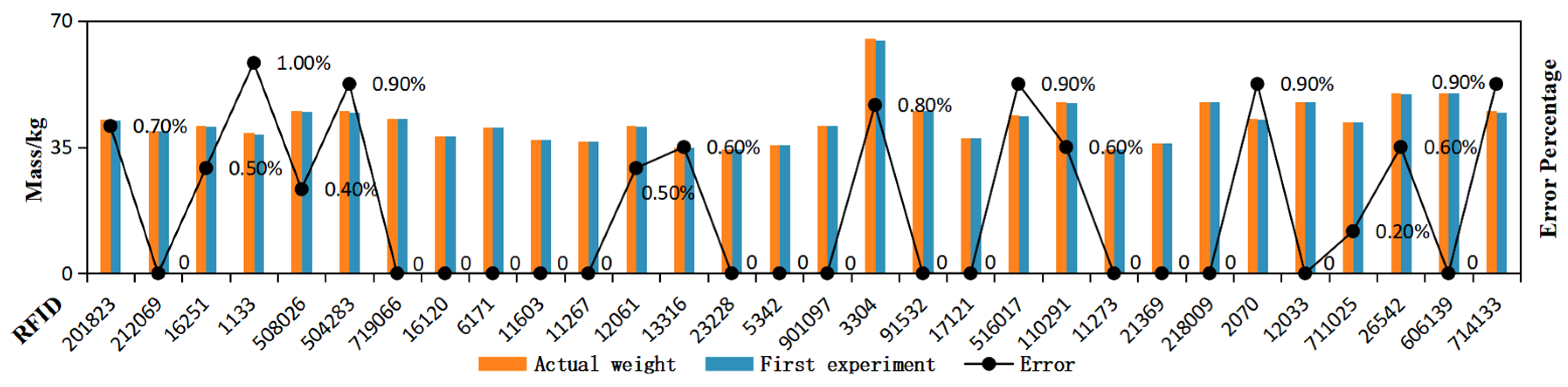
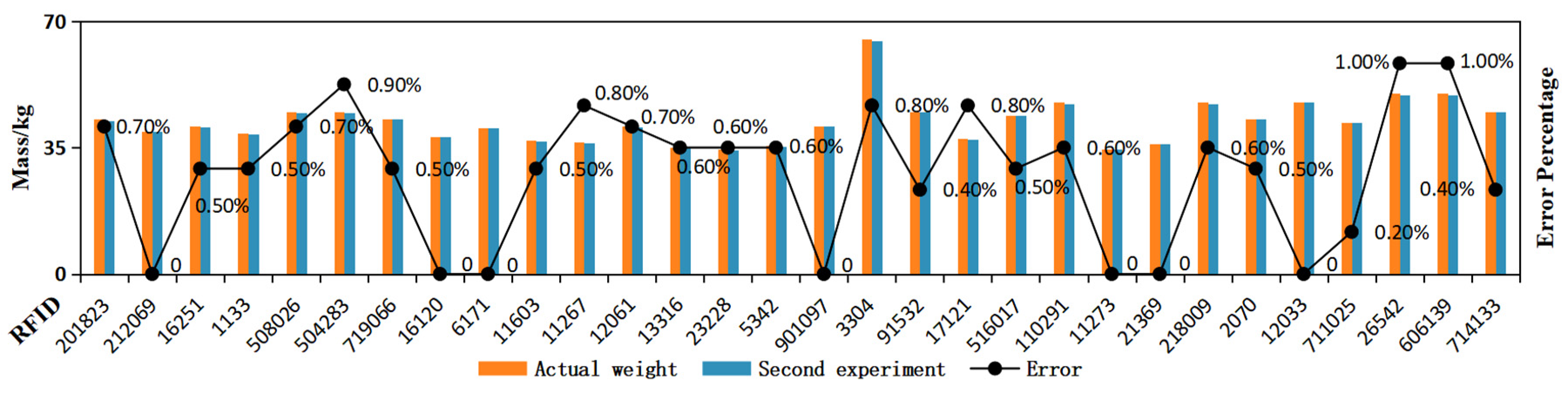
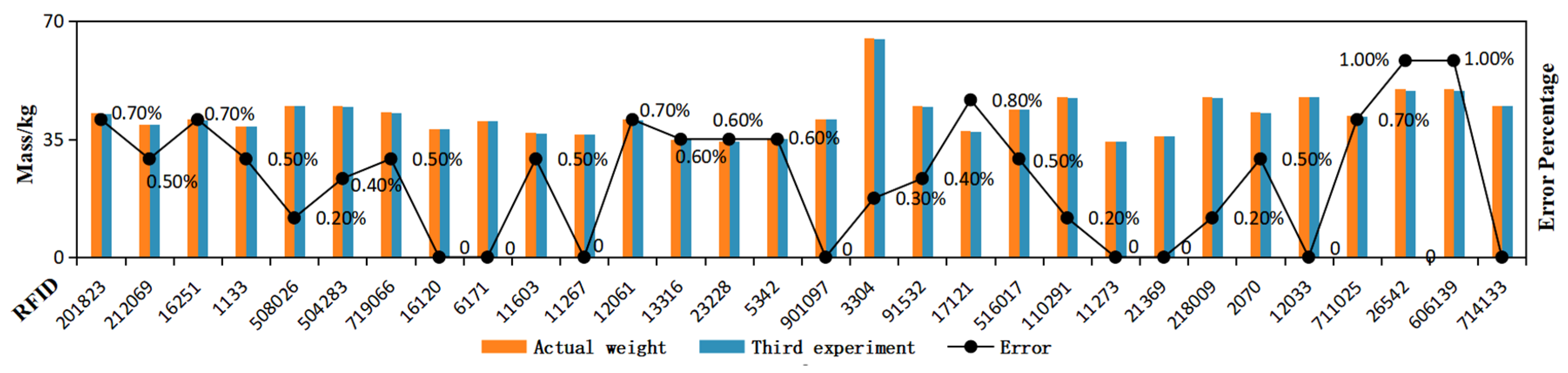
Figure 1. Workflow diagram for the channel-type sheep dynamic weighing system.
Electronics 12 01715 g001
Figure 2. Overall system structure drawing.
Electronics 12 01715 g002
Figure 3. Top view of the system.
Electronics 12 01715 g003
Figure 4. Weigh system architecture.
Electronics 12 01715 g004
Figure 5. Test hardware structure.
Electronics 12 01715 g005
Figure 6. Change diagram of the AD value under moderate activity.
Electronics 12 01715 g006
Figure 7. Array of the sliding window.
Electronics 12 01715 g007
Figure 8. Data processing.
Electronics 12 01715 g008
Figure 9. The basic process of Kalman filtering.
Electronics 12 01715 g009
Figure 10. The rendering of the Kalman filter.
Electronics 12 01715 g010
Figure 11. The rendering of EMD.
Electronics 12 01715 g011
Figure 12. The decomposition diagram of EMD.
Electronics 12 01715 g012
Figure 13. The rendering of EEMD.
Electronics 12 01715 g013
Figure 14. The decomposition diagram of EEMD.
Electronics 12 01715 g014
Figure 15. The rendering of the EEMD filter.
Electronics 12 01715 g015
Figure 16. Filter effect contrast diagram.
Electronics 12 01715 g016
Figure 17. The rendering of the Kalman-EEMD filter.
Electronics 12 01715 g017
Figure 18. Polynomial fit contrast diagram.
Electronics 12 01715 g018
Figure 19. Comparison of the ninth-order fitting and Kalman-EEMD filtering effect.
Electronics 12 01715 g019
Figure 20. Field test site. (a) The Sanbei goat farm in Erdos. Erdos, Inner Mongolia Yivi White Velvet Goat Co., Erdos Group Superfine Velvet Goat Breeding Demonstration Base. (b) Albas white cashmere goats.
Electronics 12 01715 g020
Figure 21. Site test.
Electronics 12 01715 g021
Figure 22. Data plot of the first experiment.
Electronics 12 01715 g022
Figure 23. Data plot of the second experiment.
Electronics 12 01715 g023
Figure 24. Data plot of the third experiment.
Electronics 12 01715 g024
Table 1. Field experimental data for sheep.
RFID NumberActual Weight/KgFirst/Kg RegionError Rate/%Second/KgRegionError Rate/%Third/KgRegionError Rate/%
20182342.842.5B0.7%42.5B0.7%42.5B0.7%
21206939.539.5B0.0%39.5B0.0%39.3B0.5%
01625141.040.8B0.5%40.8B0.5%40.7B0.7%
00113339.038.6B1.0%38.8B0.5%38.8B0.5%
50802645.044.8B0.4%44.7B0.7%44.9B0.2%
50428345.044.6B0.9%44.6B0.9%44.8B0.4%
71906643.043.0B0.0%42.8B0.5%42.8B0.5%
01612038.038.0B0.0%38.0B0.0%38.0B0.0%
0617140.540.5B0.0%40.5B0.0%40.5B0.0%
1160337.037.0B0.0%36.8B0.5%36.8B0.5%
01126736.536.5B0.0%36.2B0.8%36.5B0.0%
1206141.040.8B0.5%40.7B0.7%40.7B0.7%
01331635.034.8C0.6%34.8C0.6%34.8C0.6%
02322834.534.5C0.0%34.3C0.6%34.3C0.6%
534235.535.5B0.0%35.3B0.6%35.3B0.6%
90109741.041.0B0.0%41.0B0.0%41.0B0.0%
00330465.064.5A0.8%64.5A0.8%64.8A0.3%
09153245.045.0A0.0%44.8B0.4%44.8B0.4%
01712137.537.5B0.0%37.2B0.8%37.2B0.8%
51601744.043.6B0.9%43.8B0.5%43.8B0.5%
11029147.547.2A0.6%47.2A0.6%47.4A0.2%
01127334.534.5C0.0%34.5C0.0%34.5C0.0%
2136936.036.0B0.0%36.0B0.0%36.0B0.0%
21800947.547.5A0.0%47.2A0.6%47.4A0.2%
0207043.042.6B0.9%42.8B0.5%42.8B0.5%
1203347.547.5A0.0%47.5A0.0%47.5A0.0%
71102542.041.9B0.2%41.9B0.2%41.7B0.7%
02654250.049.7A0.6%49.5A1.0%49.5A1.0%
60613950.050.0A0.0%49.5A1.0%49.5A1.0%
71413345.044.6B0.9%44.8B0.4%45.0A0.0%
Disclaimer/Publisher’s Note: The statements, opinions and data contained in all publications are solely those of the individual author(s) and contributor(s) and not of MDPI and/or the editor(s). MDPI and/or the editor(s) disclaim responsibility for any injury to people or property resulting from any ideas, methods, instructions or products referred to in the content.

